

Abstract
Over the past quarter of a century the Arctic has warmed more than any other region on Earth, causing a profound impact on the Greenland ice sheet (GrIS) and its contribution to the rise in global sea level. The loss of ice can be partitioned into processes related to surface mass balance and to ice discharge, which are forced by internal or external (atmospheric/oceanic/basal) fluctuations. Regardless of the measurement method, observations over the last two decades show an increase in ice loss rate, associated with speeding up of glaciers and enhanced melting. However, both ice discharge and melt-induced mass losses exhibit rapid short-term fluctuations that, when extrapolated into the future, could yield erroneous long-term trends. In this paper we review the GrIS mass loss over more than a century by combining satellite altimetry, airborne altimetry, interferometry, aerial photographs and gravimetry data sets together with modelling studies. We revisit the mass loss of different sectors and show that they manifest quite different sensitivities to atmospheric and oceanic forcing. In addition, we discuss recent progress in constructing coupled ice-ocean-atmosphere models required to project realistic future sea-level changes.
Export citation and abstract BibTeX RIS
Invited by Mike Bevis
1. Introduction
Ice loss from the GrIS during recent years has accelerated much faster over the last two decades (Vaughan et al 2013) than current models can capture (Levermann et al 2011, Rignot et al 2011). This makes the GrIS one of the largest single contributors to sea level rise over the last decade, accounting for 0.5 out of a total of 3.2 mm yr−1 (Cazenave and Remy 2011, Anderson et al 2015, Barletta et al 2013, Groh et al 2014, Shepherd et al 2012, Jacob et al 2012, Helm et al 2014, Khan et al 2014a). If this acceleration continues, the GrIS alone could contribute as much as 9 cm of sea level rise by 2050, compared to the total sea level rise of 15–20 cm observed during the last century (Church and White 2006). Therefore, the future behavior of the GrIS is of great concern, and is also one of the largest unknowns in climate research.
GrIS mass changes are due to fluctuations in surface mass balance (SMB) processes and in ice discharge at the grounding line, both of which are dependent on atmospheric and oceanic conditions (Holland et al 2008, van den Broeke et al 2009). SMB is the difference between accumulation from precipitation (snow and rain), and mass loss from ablation (sublimation, drifting snow erosion and runoff). Dynamically-induced ice loss at the grounding line is related to accelerated flow at the marine-terminating outlets, caused by decreased buttressing and reduced basal drag that results in thinning (decreasing ice surface elevations) (Howat and Eddy 2011, Price et al 2011, Nick et al 2013). Understanding the characteristics of ice discharge and SMB prior to the last two decades (for example over the last century or millennium), combined with improved capabilities of modelling the observed short and long-term changes in Greenland's outlet glaciers, would facilitate improved predictions of future mass loss. Here we review the current state of knowledge, obtained from a variety of geodetic methods, of the GrIS mass-change over multiple timescales and its sensitivity to external forcing. We also highlight recent advances in ice-sheet modelling and what challenges need to be solved to improve ice-sheet models in future predictions.
2. Methods
Geodetic methods used to determine ice sheet volume or mass changes include airborne and satellite radar and laser altimetry (surface elevation change method), observations of ice flow of outlet glaciers using satellite interferometric synthetic-aperture radar (InSAR) (which, when combined with SMB model output, is referred to as the Input–Output method), and measurements by the Gravity Recovery and Climate Experiment (GRACE) satellite mission of changes in the gravity field caused by changes in ice sheet mass (gravimetry method). All of these methods have characteristic advantages and disadvantages. For example, airborne and satellite radar and laser altimetry have better spatial resolution than the GRACE observations, but they lack the high temporal resolution provided by the latter. Airborne and satellite radar and laser require assumptions about the firn density to convert volume to mass. In addition, satellite radar altimetry does not provide reliable results in regions of large slopes, such as those along much of the GrIS margins, and is affected by radar penetration into the snow. The Input–Output method provides the best understanding of the underlying cause of mass change in a region, but it requires knowledge of such things as outlet glacier depths, and only measures velocity along the line of site, which is problematic in many areas. Furthermore, since the net mass variations obtained using the Input–Output method are the differences between two large and, in most cases, nearly equal numbers (i.e. an SMB estimate, and an InSAR-based discharge estimate), relatively small errors in either of those numbers can lead to a relatively large error in the net mass balance. The gravimetry method provides direct estimates of mass, but has limited resolution (>250 km) and is affected by mass changes not just from ice and snow variations, but also from hydrologic and ocean mass changes, and from mass variations in the underlying solid Earth, (especially, glacial isostatic adjustment, GIA). In the remainder of this section, we provide more detailed descriptions of these methods. On local scales, other geodetic-based methods have been used to determine mass balance; for example, ground based interferometry, time lapse photography, and GPS displacement measurements of ice and bedrock. These local methods are not discussed in this paper.
2.1. Gravimetry
The GRACE mission allows for direct estimates of ice-sheet-wide mass variability, through determining the effects of that mass on the Earth's gravity field. Since its launch in March 2002, GRACE has been measuring changes in the range between two satellites that are in identical near-polar orbits (the injection altitude was 500 km), about 220 km apart. The changes in range are used to construct monthly solutions for the gravity field at the Earth's surface. Solutions are generated, for example, at the Center for Space Research (CSR) at the University of Texas (Tapley et al 2004), the Jet Propulsion Laboratory (JPL) at the California Institute of Technology (Landerer et al 2012) and the Deutsches GeoForschungsZentrum (GFZ) at Helmholtz Centre Postdam (Kusche et al 2009). The gravity fields consist of spherical harmonic (Stokes) coefficients, Clm and Slm, where l and m denote the degree and order of the harmonic coefficients, respectively; though most users replace the GRACE C20 coefficients with C20 estimates inferred from satellite laser ranging (Cheng and Tapley 2004).
The GRACE gravity solutions allow users to determine monthly mass fluctuations averaged over scales of a few hundred km and greater. Mass variability from individual glaciers, though, cannot be resolved. The contributions from all glaciers within a region are automatically included in a regional estimate, but it is not possible to determine how much each glacier contributed (Velicogna et al 2014). Unlike other methods, GRACE provides a direct estimate of mass balance, without requiring any intermediate assumptions (other than Newton's Law of Gravity). However, the GRACE gravity fields represent the total gravity variability from all geophysical sources, and cannot distinguish between contributions from ice sheet mass, and those from such things as mass variations within the atmosphere, ocean, and liquid water storage on land; or from signals associated with mass variability in the solid Earth: e.g. episodic (earthquake) processes, and glacial isostatic adjustment (the viscoelastic response of the solid Earth to glacial unloading over the last several thousand years) (Sutterley et al 2014). For Greenland, none of these other sources of gravity is likely to be a serious problem. The GRACE centers use model output to remove atmospheric and oceanic signals before constructing the monthly gravity fields. Greenland is far enough from other land areas that the effects of liquid land water storage do not cause appreciable contamination of the Greenland results. And, Greenland and the surrounding region do not experience earthquakes that are large enough to significantly affect the Greenland mass estimates. The GIA signal is potentially more of an issue. Since it is linear and cannot be separated from a linear trend in present-day ice mass, it should be independently modelled and removed. However, existing GIA models suggest that this correction is rather small for Greenland, about −7 ± 19 Gt yr−1 (Velicogna and Wahr 2006).
Figure 1 shows the average rate of mass change across the GrIS between April, 2002 and July, 2014, determined from the CSR GRACE fields. The GRACE C20 gravity coefficients are replaced with those estimated from satellite laser ranging (Cheng and Tapley 2004). Degree-one coefficients are also included, computed as described by Swenson et al (2008). The method described in Wahr et al (1998) is used to transform the gravity coefficients into surface mass coefficients. Those coefficients are used to compute surface mass on a 0.5 × 0.5 degree grid, smoothed with a Gaussian smoothing function with a 250 km half-width. Figure 2 shows the time series of the total mass change for the GrIS, estimated from GRACE monthly mass solutions for the period from April, 2002 to June, 2014.

Figure 1. Average April 2002–June 2014 mass change rate of the Greenland ice sheet extracted from GRACE, in units of centimetres per year of equivalent water thickness.
Download figure:
Standard image High-resolution image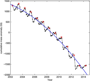
Figure 2. Time series of the cumulative ice sheet-wide mass anomaly of the GrIS extracted from GRACE, in gigatonnes. The red asterisks denote June values (or May values, for years when June is missing), and best-fitting trend quadratic trend (blue).
Download figure:
Standard image High-resolution image2.2. Surface elevation changes
Airborne or satellite-borne radar or laser sensors are used to repeatedly map glacier surface elevations to estimate volume changes. The technique can provide a detailed pattern of mass imbalance for major drainages and glaciers.
2.2.1. Satellite laser altimetry.
Satellite laser altimetry from the Geoscience Laser Altimeter System (GLAS) instrument on the Ice, Cloud, and land Elevation Satellite (ICESat) provided global measurements of surface elevation from 2003 to 2009, and repeated those measurements along almost identical tracks (separated by a few hundred meters), typically 2–3 times a year. The primary goal of the mission was to measure changes in ice volume over time.
The latest ICESat Release 34 data (Zwally et al 2014) are available from the National Snow and Ice Data Center (https://nsidc.org/data/icesat/). The level-2 altimetry product (GLA12) provides surface elevations for ice sheets and consists of 18 campaigns. The satellite laser footprint diameter is 30–70 m and the distance between footprint centres is approximately 170 m. The dominant biases come from pointing errors and saturation errors. For ICESat elevations that have been corrected for both pointing and saturation errors, and that have been filtered for surface roughness and atmospheric scattering and corrected for intercampaign elevation biases (Hofton et al 2013, Borsa et al 2014), the single-shot accuracy is σICESat = 0.1 m. Figure 3 shows elevation change rates during 2003–2009 derived from ICESat.

Figure 3. Elevation change rates during 2003–2009, as derived from ICESat.
Download figure:
Standard image High-resolution image2.2.2. Airborne laser altimetry
Land, vegetation, and ice sensor (LVIS).
NASA's Land, Vegetation, and Ice Sensor (LVIS) is a scanning laser altimeter instrument that provides data on surface topography and vegetation coverage. LVIS has a scan angle of about 12 degrees, and can cover about 2 km swaths of surface from an altitude of 10 km. LVIS flew aboard the DC-8 and P-3B airborne laboratories until 2011, and since then in a King Air B-200, a Gulfstream G-V and an HU-25C Guardian Falcon. LVIS data were collected as part of NASA funded campaigns and are available from 2009 to 2013 through the National Snow and Ice Data Center (http://nsidc.org/data/ilvis2). Data from a single pre-IceBridge campaign in 2007 are available from http://nsidc.org/data/blvis0. Figure 4 shows the surface elevation over the frontal portion of Jakoshavn Isbræ in west Greenland. The high pixel resolution of LVIS allows detection of small icebergs in the Kangia Fjord. LVIS can be used to validate and calibrate measurements by, for example, ICESat (Hofton et al 2008) and CryoSat-2 elevations.
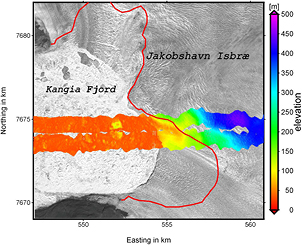
Figure 4. Surface elevation over the Jakobshavn Isbræ measured by LVIS in 2007. The background shows SPOT imagery from August 2007. The red curve represents the calving front in August 2013.
Download figure:
Standard image High-resolution imageAirborne topographic mapper (ATM).
The ATM, developed at NASA's Wallops Flight Facility (WFF) in Virginia, is a scanning laser altimeter that measures ice surface elevation from an aircraft at an altitude of between 400 and 800 m above ground level. NASA has flown ATM surveys in Greenland nearly every year since 1993 aboard the NASA DC-8, twin-otters (DHC-6), C-130's, and other P-3 aircraft. The ATM has been participating in NASA's Operation IceBridge since 2009. The NASA IceBridge and pre-IceBridge ATM Level-2 Icessn Elevation, Slope, and Roughness (BLATM2) data from 1993 to 2013 are available through the National Snow and Ice Data Center (http://nsidc.org/data/ilatm2).
ATM flights are mainly concentrated along the main flowlines of outlet glaciers. In particular, the frontal portion of Jakobshavn Isbræ has been very well surveyed over the last two decades. The ATM measurements have an elevation accuracy of σATM = 0.1 m (Krabill et al 2002).
Merging ICESat, ATM, and LVIS.
Ice loss from the GrIS is dominated by loss in the marginal areas. Dynamically-induced ice loss and the associated ice surface lowering is often largest close to the glacier calving front and may vary from rates of tens of meters per year to a few meters per year over relatively short distances (5–10 km) (Howat et al 2007, Stearns and Hamilton 2007, Liu et al 2012). Hence, high spatial resolution data are required to accurately estimate volume changes. To improve volume change estimates, especially those caused by marginal thinning, ICESat data may be supplemented with, for example, altimeter surveys from ATM and LVIS (Kjeldsen et al 2013, Schenk et al 2014). A recent study by Kjeldsen et al (2013), shows a difference of about 11% between ice loss estimates obtained using ICESat data solely, and using ICESat data supplemented with airborne laser data from ATM and LVIS. Other studies, for instance Howat et al (2008), supplement ICESat derived surface elevation changes with differenced Advanced Spaceborne Thermal Emission and Reflection (ASTER) radiometer digital elevation models of outlet glaciers in southeastern Greenland, to obtain improved regional volume-loss rates.
2.2.3. Satellite radar altimetry.
Radar altimetry provides ice-sheet volume changes from surface elevation changes. Among all geodetic techniques satellite radar altimetry provides the longest continuous record of ice-sheet-wide volume changes. The European Space Agency's (ESA) European Remote Sensing 1 and 2 (ERS-1 and ERS-2) satellite radar altimeters and the Environmental Satellite (Envisat) radar provide ice-sheet-wide observations of surface changes from May 1992 to September 2010. The Envisat altimeter, launched in April 2002 followed the same 35 d orbit as ERS-1 and ERS-2 to ensure a homogeneous time series over more than two decades (Remy and Parouty 2009, Khvorostovsky 2012).
To obtain surface elevations, corrections are applied for the lag of the leading-edge tracker, surface scattering, dry atmospheric mass, water vapour, ionosphere, slope-induced error, solid Earth tide, and ocean loading tide (Wingham et al 1998, Davis and Ferguson 2004, Remy and Parouty 2009, Khvorostovsky 2012). Biases between waveform parameters are estimated to create their time series along with time series of surface elevation change for determining correction, which account for the correlation between backscattered power and surface elevation change (Davis and Ferguson 2004, Wingham et al 2008, Remy and Parouty 2009, Khvorostovsky 2012). Radar altimetry suffers from problems with surface slope; therefore, great caution should be made when using data over coastal regions with rough terrain. Furthermore, the scale of outlet glaciers in Greenland (5–10 km wide) is small in comparison to the size of the pulse-limited altimeter footprint (nominally 2–10 km in diameter), which leads to significantly reduced data volumes in the ice marginal regions. Additionally, when merging ERS-1, ERS-2 and Envisat data, inter-satellite biases have to be estimated and removed (Khvorostovsky 2012).
2.2.4. Ice volume to mass.
The conversion of a volume loss rate obtained from any of the above altimetric techniques, into a mass loss rate, requires assumptions about density. To estimate elevation changes due to firn compaction, recent studies have used a simple firn model (Li and Zwally 2011, Zwally et al 2011, Khan et al 2014a) that includes melt and refreezing (Reeh 2008). The firn model is forced by annual temperature, accumulation, melt, and refreezing from one of several regional models, such as BOX (Box 2013, Box et al 2013), MAR (Fettweis et al 2011), RACMO2 (Ettema et al 2009), HIRHAM (Christensen et al 2006), or the model by Hanna (Hanna et al 2011). Figure 5 shows elevation change rates due to firn compaction as a function of time using temperature, accumulation, melt, and refreezing from the regional climate model RACMO2 (Khan et al 2014). The height changes due to firn compaction correspond to ice-sheet-wide volume changes of −11.9 ± 3.4 km3 yr−1 during 2003–2006, −29.8 ± 3.4 km3 yr−1 during 2006–2009, and −41.0 ± 3.4 km3 yr−1 during 2009–2012. Other studies, for example Sørensen et al (2011), used forcing from the HIRHAM5 regional climate model (Christensen et al 2006) and obtained ice-sheet-wide firn correction of −19 km3 yr−1 for 2003–2008. For comparison, using the model of Khan et al (2014a) gives an average firn correction for 2003–2008 of −18 km3 yr−1.
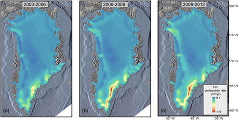
Figure 5. Elevation change rates due to firn compaction during (a) 2003–2006, (b) 2006–2009, and (c) 2009–2012 using climate inputs from RACMO2.
Download figure:
Standard image High-resolution image2.2.5. Correction for elastic uplift of the bedrock.
Observed ice surface elevation changes must be corrected for bedrock movement caused by elastic uplift from present-day mass changes (Khan et al 2010b, Bevis et al 2012). To demonstrate the order of this correction and its evolution over time, we use mass loss estimates from Khan et al (2014a) and convolve with Green's function for vertical displacements derived by Boy (Petrov and Boy 2004) for the Preliminary Reference Earth Model (Dziewonski and Anderson 1981). Figure 6 shows predicted vertical deformation of bedrock during 2003–2006, 2006–2009, and 2009–2012, respectively. The correction due to elastic uplift converted to ice volume corresponds to 3.6 ± 0.3 km3 yr−1 during 2003–2006, 8.2 ± 0.3 km3 yr−1 during 2006–2009, and 9.9 ± 0.4 km3 yr−1 during 2009–2012.
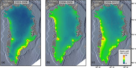
Figure 6. Predicted elastic uplift of the bedrock due to present-day ice loss during (a) April 2003–April 2006, (b) April 2006–April 2009, and (c) April 2009–April 2012.
Download figure:
Standard image High-resolution image2.2.6. Correction for glacial isostatic adjustment.
Ice surface elevation changes must be corrected for the viscous response of the lithosphere to past glacial history, or glacio-isostatic adjustment. Figure 7 shows uplift rates derived from ICE-5G (VM2 L90) model version 1.3 (Peltier 2004). Grid data files are available from (www.atmosp.physics.utoronto.ca/~peltier/data.php). Rates of vertical land motions caused by GIA can be considered constant over an inter-decadal timescale. We obtain an ice-sheet-wide GIA correction, that converts to an ice volume of −0.1 km3 yr−1. When considering ice-sheet-wide volume loss, the positive rates in north Greenland (uplift of about 8 mm yr−1) seem to largely cancel the negative values in central Greenland (subsidence of about 4 mm yr−1), resulting in an overall small GIA correction of −0.1 km3 yr−1. However, over smaller regions, for example the northeast sector of the GrIS, the GIA correction is 0.9 km3 yr−1. Other GIA models, for example HUY2 (Simpson et al 2011), give a similar ice-sheet-wide correction of <1 km3 yr−1.

Figure 7. Predictions of GIA uplift rates in mm/yr derived using ICE-5G.
Download figure:
Standard image High-resolution image2.3. The input–output method
The input–output method quantifies the difference between the SMB and ice discharge, D, at the grounding line (van den Broeke et al 2009).

Consequently, the method provides estimates of SMB and discharge separately at individual glacier drainage basins (Rignot and Kanagaratnam 2006, Howat et al 2007, Rignot et al 2008, van den Broeke et al 2009).
SMB is constructed from regional atmospheric climate models and provides sub-daily predictions at high spatial resolution. The SMB model errors depend on the location and size of the study area. Errors are typically 5–20%. However, larger errors are likely in areas with extreme precipitation or melting (low or high). One other important issue is the general assumption of the altitude of the 'grid-cell' under consideration when downscaling numerical climate model. This can often provide major errors. Model resolutions typically range from approximately 10 to 30 km or more.
To estimate D it is necessary to measure ice velocity and ice thickness. However, often no measurement of ice thickness at the glacier grounding line is available, and so

where δDg is the ice storage due to glacier dynamics between the flux gate and the grounding line, and δSMBg is the SMB anomaly between the flux gate and the grounding line. The ice flux through a flux gate is,

where ν is the gate-perpendicular ice surface velocity and f is the mean ratio of surface to depth-averaged velocity, ρ is the ice density, and w and h are the width and height of the ice column.
To estimate the ice sheet mass anomaly, δM, the time-integrated (cumulative) anomalies of δSMB and δD are required (Broeke et al 2009),
with SMB0 and D0 the reference surface mass balance and discharge.
Velocity maps are derived from, for example, InSAR data from the RADARSAT-1 satellite. Measurements are obtained from overlapping images and represent the mean velocity over days to months. The formal errors determined from radar-derived speeds compare very well with those derived from GPS data (Joughin 2002). In general, formal errors are well below the observed speeds of glacier change. However, velocity maps are also derived by applying feature tracking between pairs of optical images (for example Landsat-5 TM Band 4 and Landsat-7 ETM+ Band 8). For some outlet glaciers, e.g. Helheim Glacier, Kangerdlugssuaq Glacier, and Jakobshavn Isbræ, the velocity is mapped at a high frequency (approximately monthly) (Howat et al 2011, Bevan et al 2012), allowing sub-annual estimation of ice discharge. The largest uncertainty in ice discharge calculations comes from areas of no or very poor ice thickness observations. The recent bed map of Bamber et al (2013a) derived from a combination of multiple airborne ice thickness surveys undertaken between the 1970s and 2012 has made significant improvements. However, areas with only a few measurements are still present. Further advances in improving bed topography have recently been made by applying a mass conservation scheme which incorporates surface velocity measurements and radar measurements of the bed (Morlighem et al 2014). Overall, errors in bed elevation range from a minimum of ±10 m to about ±300 m Bamber et al (2013a). For many outlet glaciers, the thinning rate over the last decade has increased to >10 m yr−1; thus, the temporal evolution of ice thickness has to be taken into account for precise ice flux estimation. Furthermore, flow speed, and therefore discharge, can vary significantly on sub-annual timescales (Howat et al 2007, Joughin et al 2008, Howat et al 2011). Therefore, Sub-annual velocity maps may improve mass change rates. A snapshot of a few velocity maps may under-sample the discharge signal and yield incorrect cumulative changes in mass (Howat et al 2011).
3. Ice mass changes over multiple timescales
3.1. Catchment-wide mass loss during last decade
To study the spatial and temporal variability of the mass change components, we divide the GrIS into a set of major drainage basins numbered from 1 to 8 (see figure 8) representing (1) north, (2) northeast, (3) east, (4) southeast, (5) south, (6) southwest, (7) west, and (8) northwest. These major basins are further divided into sub-drainage basins (see figure 8).

Figure 8. Map of observed surface speeds from Joughin et al (2010) and the major drainage basins. Arrows denote the Irminger current (red), the East Greenland current (blue arrow), and the West Greenland current (orange arrow).
Download figure:
Standard image High-resolution imageThe ice-sheet and catchment-wide mass balance estimates have been greatly improved over the past few decades by the use of satellite geodesy measurements. Observations show a significant increase in ice loss associated with the speed up of glaciers in southeast and northwest Greenland starting in 2003 and 2005, respectively, followed by a slowdown of ice speed between 2006 and 2009. These short-term perturbations have a significant impact on the mass balance averaged over decadal scales. To illustrate the temporal and spatial variability of the GrIS over the last two decades, we consider the mass change in each major drainage basin defined in figure 8.
Southeast: since 2000, the rates of discharge from several marine-terminating glaciers along the southeast coast, notably Kangerdlugssuaq (basin 3.3), Helheim (basin 4.1), and the many glaciers in basin 4.2, have more than doubled as a result of significant accelerations in flow speed (Rignot and Kanagaratnam 2006) (see figures 9 and 10). The sudden speed-ups of those glaciers coincided with observed thinning rates of 15–90 m yr−1 (Joughin et al 2004, Howat et al 2005, 2008, Stearns and Hamilton 2007), which indicates a significant mass imbalance in this area of the ice sheet. Recent studies suggest increased melt-induced ice loss over the last decade, and an almost equal split between surface processes and ice discharge in this region (van den Broeke et al 2009, Sasgen et al 2012). However, in the last few years (2009–2012) the rate of discharge has decreased (Enderlin et al 2014).

Figure 9. Mass change estimates for Greenland's major drainage basins.
Download figure:
Standard image High-resolution image
Figure 10. Rates of total ice mass change, the SMB component, and the dynamic component during 2003–2006, 2006–2009, and 2009–2012 (Khan et al 2014a). Red circles denote mass loss, and green circles denote mass gain.
Download figure:
Standard image High-resolution imageIn southwest Greenland (drainages 6.2 and 6.1), where the ice sheet margin is typically located up to 100 km inland of the coastline, there are few marine terminating glaciers and ice loss is dominated by atmospheric forcing (van den Broeke et al 2009, Wake et al 2009, Tedesco et al 2013). The ice sheet has a gentler slope compared to the southeast coast, and surface melting occurs much farther inland. The few glaciers terminating in long fjords do, however, also undergo dynamic thinning, but to a lesser degree than the marine terminating glaciers in the northwest and southeast. Such has been the case for the Sermilik Bræ (drainage zone 5), whose mass loss in the second half of the twentieth century was equally split between an SMB anomaly and a discharge anomaly (Podlech et al 2004). The large marine terminating glacier Kangiata Nunata Sermia (KNS) has also been a major contributor to dynamic-induced driven mass loss in the region (drainage basin 6.2), undergoing speed up and thinning in 2010 (Van As et al 2014).
Jakobshavn Isbræ (basin 7.1) in west central Greenland has long been regarded as Greenland's fastest-flowing glacier, and drains about 6% of the GrIS area (Motyka et al 2010). The floating ice tongue has been retreating for more than a century (Csatho et al 2008), resulting in increased discharge. The largest observed rapid retreat and massive ice loss began in 1998 (Motyka et al 2010). Recently speeds of more than 17 km yr−1 have been recorded, making it the fastest glacier in both Greenland and Antarctica (Joughin et al 2014b). The influence of warm oceanic water on the calving glacier front has been a driver for episodes of rapid retreat and speed-up (Holland et al 2008). It is believed that the glacier will continue to undergo episodes of rapid dynamic changes, because the front has presently reached an overdeepening, allowing further retreat (Morlighem et al 2013, Joughin et al 2014b). Model studies show that Jakobshavn Isbræ is likely to continue its high rate of mass loss into the future, with substantial contributions from both increased SMB-induced mass loss and increased ice discharge (Price et al 2011, Nick et al 2013).
The northwest coast of Greenland (drainage zone 8.1) has received much attention due to large mass losses observed in the early twenty first Century (Rignot et al 2008, Khan et al 2010a). This region of the ice sheet is dominated by vast contact with the ocean—there is very little land, and the ice sheet terminates directly into the ocean. Presently the mass loss is equally split between an SMB anomaly and a discharge anomaly, whereas previous rapid mass loss events were entirely dominated by ice dynamics (Kjær et al 2012). Historical aerial photographs from this region show that this region has experienced rapid increases and decreases in discharge (Kjær et al 2012), just as has been observed in other regions where the mass loss is heavily affected by oceanic conditions (Howat et al 2007, Nick et al 2009).
North sector:in contrast to the southwest, Greenland's north sector (drainage basin 1) is characterised by major marine-terminating outlet glaciers. These glaciers are surrounded by year-round sea ice and a thick ice mélange, which appears to suppress calving front retreat (Amundson et al 2010, Seale et al 2011, Christoffersen et al 2012, Schild and Hamilton 2013). Occasionally the sea-ice breaks up, leaving the outlets open to oceanic forcing, which may lead to large calving events (Higgins 1991, Reeh et al 2001). The Petermann Glacier is among the largest of the Greenlandic outlets, with the second largest floating shelf (Rignot et al 2001). Unlike most other glaciers in Greenland, the majority of the mass loss (~80%) occurs as submarine melt. In 2010 a very large calving event occurred, removing ~25% of the glacier tongue (Falkner et al 2011, Nick et al 2012). The calving is likely a part of a natural cycle, and did not lead to increased mass loss or speed-up of the ice stream (Falkner et al 2011, Nick et al 2012). This sector of the ice sheet has a negative SMB anomaly. And while the SMB anomaly has varied throughout the last decade, the discharge component has remained stable (Khan et al 2014a).
In the northeast sector (drainage basins 2.1 and 2.2) there have been observations of increased discharge and melting. This sector is occupied by the prominent North East Greenland Ice Stream (NEGIS), which drains into the outlets of the 79 Fjord glacier, Zachariae Isstrøm, Storstrømmen, and Bidstrup Glacier. The former two outlet glaciers have both lost large amounts of ice through increased discharge starting during the period 2003–2006 and continuing into the present (Khan et al 2014a).
3.2. Ice-sheet-wide mass changes since 1978
By comparing recent estimates of the GrIS mass balance with those since the early 1990s, its evident that mass loss from the ice sheet has more than doubled during the past quarter of a century (figure 11). Estimates of the state of the GrIS include those derived from space-borne radar altimetry, air-and space-borne laser altimetry, satellite gravimetry, the input–output method, and very often a combination of more than one type of measurement (references are given in table 1). See section 2 for a description of the methods.
Table 1. Mass loss rates: rate of mass change of the GrIS derived from different methods.
| Source and Year | Technique | Time range | Mass loss rate Gt yr−1 | Notes |
|---|---|---|---|---|
| Radar | ||||
| Zwally et al (2005) | SRALT (ERS 1–2) + limited ATM | 1992–2002 | 11 ± 3 | Satellite radar altimetry is affected by surface slope near ice margins and changes in penetration |
| Johannessen et al (2005) | SRALT (ERS 1–2) low elevations sparsely sampled | 1992–2003 | 30 ± 3 | Densities of 0.9, 0.5, 0.4, 0.3, 0.3 Gt km3 assumed to convert area-weighted height change in elevation into mass intervals (<1.5, 1.5–2, 2–2.5, 2.5–3, >3 km) |
| Zwally et al (2011) | SRALT (ERS 1–2) + limited ATM | 1992–2002 | −7 ± 3 | Superseeds Zwally et al (2005) |
| Hurkmans et al (2014) | 1996–2001 | 5.5 ± 32.1 | ||
| Air- and space-borne laser altimetry | ||||
| Krabill et al (2004) | ATM | 1993–1998 | −55 ± 3 | |
| 1997–2003 | −73 ± 11 | |||
| Thomas et al (2006) | ATM | 1993–1998 | −27 ± 24 | High end of range likely due to limited coverage at low elevations |
| ATM/ICESat | 1998–2004 | −81 ± 24 | High end of range likely due to limited coverage at low elevations | |
| Slobbe et al (2009) | ICESat | 2003–2007 | −139 ± 68 | Used large density range (±300 kg m3) for error bounds |
| Zwally et al (2011) | ICESat | 2003–2007 | −174 ± 4 | |
| Sørensen et al (2011) | ICESat | 2003–2008 | −233 ± 27 | |
| 2003–2008 | −191 ± 23 | |||
| 2003–2008 | −240 ± 28 | |||
| Ewert et al (2012) | ICESat | 2003–2008 | −181 ± 28 | |
| Sasgen et al (2012) | ICESat | 2003–2009 | −245 ± 28 | |
| Khan et al (2014a) | ATM + LVIS + ICESat | 2003–2006 | −172.4 ± 21,7 | |
| 2006–2009 | −292 ± 23,2 | |||
| 2009–2012 | −359.8 ± 28,9 | |||
| Hurkmans et al (2014) | ICESat | 2003–2008 | −234.8 ± 46.9 | |
| Input–Output method | ||||
| Rignot and Kanagaratnam (2006) | InSAR (ice motion) 1996 + balance anomaly estimate (Hanna et al 2005) | 1996–1997 | −83 ± 28 | |
| InSAR (ice motion) 1996 + balance anomaly estimate (Hanna et al 2005) | 2000–2001 | −127 ± 28 | ||
| InSAR (ice motion) 1996 + balance anomaly estimate (Hanna et al 2005) (extrapolated) | 2005–2006 | −205 ± 38 | ||
| van den Broeke et al (2009) | InSAR-RACMO | 2003–2008 | −237 ± 20 | |
| Sasgen et al (2012) | InSAR-RACMO | 2003–2009 | −260 ± 58 | |
| Enderlin et al (2014) | SMB—D | 2000–2005 | −153 ± 33 | |
| 2005–2009 | −265 ± 18 | |||
| 2009–2012 | −378 ± 50 | |||
| Langer et al (2014) | SMB—D | 2007–2011 | −262 ± 21 | |
| GRACE | ||||
| Chen et al (2006) | GRACE—averaging filter applied to monthly spherical harmonic gravity field product | 2002–2005 | −219 ± 21 | |
| Luthke et al (2006) | GRACE MASCON—(change in gravitational acceleration on each orbital pass fit to forward model of mass history of local basins) | 2003–2005 | −101 ± 16 | Gain of 54 Gt yr−1 above 2000 m and loss of 155 Gt yr−1 below 2000 m |
| Velicogna and Wahr (2006) | GRACE—averaging filter applied to monthly spherical harmonic gravity field product | 2002–2006 | −227 ± 33 | |
| Ramillien et al (2006) | GRACE—averaging filter applied to 10 d gravity solutions | 2002–2005 | −118 ± 14 | |
| Wouters et al (2008) | GRACE EOF decomposition of monthly spherical harmonics iteratively fit with forward model of mass change of basins (based initially on R&K and iterated) | 2003–2008 | −179 ± 25 | |
| 2003–2005 | −121 ± 27 | Same period as Luthke et al (2006) similar elevation dependence seen | ||
| 2006–2008 | −204 ± 25 | Range in net balance is range of results using gravity products from four diff erent centers, rather than estimated error | ||
| Slobbe et al (2009) | GRACE using products from CNES (Centre National d'Etudes Spatiales), CSR (Center for Space Research, University of Texas-Austin), DEOS (Delft Institute of Earth Observation and Space Systems, Delft University of Technology, Delft), and GFZ (GeoForschungsZentrum, Helmholtz-Zentrum Potsdam) | 2002–2007 | −173 ± 45 | Range: −128 to −218 Gt yr−1 |
| Velicogna (2009) | GRACE | 2002–2009 | −230 ± 33 | |
| Ewert et al (2012) | GRACE—GFZ | 2002–2009 | −191 ± 21 | |
| Sasgen et al (2012) | GRACE | 2003–2009 | −238 ± 29 | |
| Siemes et al (2013) | GRACE—DEOS | 2003–2004 | −129 ± 15 | |
| 2005–2006 | −146 ± 17 | |||
| 2007–2008 | −209 ± 29 | |||
| 2003–2008 | −165 ± 15 | |||
| Barletta et al (2013) | GRACE | 2003–2011 | −234 ± 20 | |
| 2003–2008 | −211 ± 23 | |||
| 2002–2007 | −179 ± 22 | |||
| 2007–2011 | −276 ± 27 | |||
| Velicogna and Wahr (2013) | GRACE | 2003–2012 | −258 ± 41 | |
| Wouters et al (2013) | GRACE | 2003–2012 | −249 ± 20 | |
| Khan et al (2014a) | GRACE | 2003–2006 | −205 ± 20,2 | |
| 2006–2009 | −256.6 ± 21,8 | |||
| 2009–2012 | −359.8 ± 20,3 | |||
| The ice sheet mass balance inter-comparison exercise (IMBIE) | ||||
| Shepherd et al (2012) | Reconciled estimate from radar, laser altimetry, input–output, and GRACE | 1992–2012 | −142 ± 49 | |
| 1992–2000 | −51 ± 65 | |||
| 1993–2003 | −83 ± 63 | |||
| 2000–2011 | −211 ± 37 | |||
| 2005–2010 | −263 ± 30 | |||
| 2003–2008 | −232 ± 23 | |||
| Empirical relations between surface mass balance and ice discharge | ||||
| Rignot et al (2008) | Regression between SMB-anomalies with ice discharge | 1960–1970 | −110 ± 70 | |
| 1970–1990 | −30 ± 50 | |||
| 1996 | −97 ± 47 | |||
| 2000 | −156 ± 44 | |||
| 2004 | −231 ± 40 | |||
| 2005 | −293 ± 39 | |||
| 2006 | −265 ± 39 | |||
| 2007 | −267 ± 38 | |||
| Yang (2011) | Regression between inter-annual anomalies in modeled melt-index and ice discharge estimates from Rignot and Kanagaratnam (2006) | 1958–2007 | −170 ± 50 | |
| 1961–2003 | −167 ± 50 | |||
| 1993–2003 | −163 ± 47 | |||
| 1996–2007 | −213 ± 56 | |||
| Box and Colgan (2013) | Regression between 13 year smoothed runoff and ice discharge | 1840–2010 | −52.6 ± 21,0 | |
| Energy- and climate modeling | ||||
| Van de Wal and Oerlemans (1994) | Energy balance modeling | 1890–1990 | −90 ± 46,8 | |
| Zuo and Oerlemans (1997) | Glacier mass balance and climate modeling | 1865–1990 | −86.4 ± 25,2 |
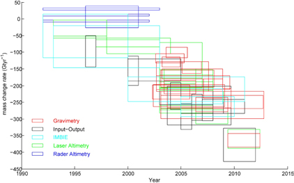
Figure 11. Mass changes during 1992–2012. Colours refer to the different methods used to derive estimates. The x and y directions of the squares denote the time intervals and uncertainties of the mass loss rate. See table 1 for references.
Download figure:
Standard image High-resolution imageThe period from the 1990s to the beginning of the twenty-first century was characterised by a relatively small mass loss. At higher elevations above 2000 m the ice sheet was in balance and even thickening, while at lower elevation the periphery was thinning (Krabill et al 1999, 2000, Zwally et al 2011). During the 1990s the SMB contribution to the mass loss increased, owing to a larger surface melt with precipitation that remained constant. Ice discharge also increased during this period, and total annual mass loss rates of 51 Gt yr−1 were reported for the GrIS from 1994 to 1999 (Rignot et al 2011).
In northeast and northwest Greenland the observational record was recently extended back to 1978 and 1985, respectively, using aerial stereo-photogrammetric imagery that provided new information on ice dynamics. In northeast Greenland the ice margin remained stable from 1978 until ~2003, at which time the ice loss started to rapidly increase. The ice loss has accelerated continuously since 2003 (Khan et al 2014). In northwest Greenland aerial imagery combined with geodetic observations revealed two periods of considerable dynamic-induced ice loss from the ice sheet margin, namely 1985–1993 and 2005–2010, while mass loss during the intervening period was governed by SMB-induced changes (Kjær et al 2012, Khan et al 2013).
3.3. Long-term mass changes (century timescale)
Modern aerial and satellite observations allow measurements of volume and mass change at various temporal and spatial scales. However, these are confined to recent decades. In recent years several studies have focused on changes in front positions of outlet glaciers during the satellite-era from the 1970s and onwards at various temporal and spatial scales (Moon and Joughin 2008, Box and Decker 2011, Howat and Eddy 2011, McFadden et al 2011, Carr et al 2013). Mapping the front position over sufficiently long timescales may provide information about the outlet glaciers dynamic response to slowly changing external forcings.
To extend the observational record of surface lowering and glacier front positions to the century timescale, back beyond the satellite-era, a range of different methods has been applied. These include the use of historical maps and reports from early expeditions to Greenland during the nineteenth and twentieth centuries, aerial imagery from the 1930s and onwards, and identification of the Little Ice Age extent on contemporary aerial and satellite-imagery (Andresen et al 2014, Weidick 1959, 1994, Podlech et al 2004, Csatho et al 2008, Bjørk et al 2012, Kelley et al 2012, Lecleqer et al 2014, Lea et al 2014, Khan et al 2014b). The Little Ice Age was a period of cooling that occurred from about 1350 to about 1850. The maximum ice extent during the Little Ice Age is identified using the so-called 'historical moraines', i.e. fresh non-vegetated moraines close to the present glacier fronts seen in many parts of Greenland, and fresh trimlines, i.e. pronounced boundaries between abraded and less-abraded bedrock on valley sides (Csatho et al 2008, Khan et al 2014b; see also figure 12). These mark the culmination of the Little Ice Age glacier advances.

Figure 12. Glacier front positions of Jakobshavn Isbræ (a), Kangerdlugssuaq Glacier (b), and Helheim Glacier (c). Glacier front positions are based on historical maps from early expeditions, aerial imagery from the 1930s and onwards, and satellite observations. The background map is a Landsat7 ETM+ 'true color' image.
Download figure:
Standard image High-resolution imageIn general, Greenland outlet glaciers respond rapidly to atmospheric and oceanic forcing. For example warming during the 1920s and 1930s caused retreat of glaciers, while slowing down or even re-advance occurred during the cooler mid-twentieth century (Andresen et al 2014, Weidick 1994, Bjørk et al 2012). However, despite overall regional trends, adjacent outlet glaciers may have reacted differently during the twentieth century after being subjected to the same external forcing, thus underlining the important impact of bathymetric and topographic control (Andresen et al 2014, Warren and Glasser 1992, Weidick 1994, Bjørk et al 2012, Kelley et al 2012, Enderlin et al 2013). An example of this is the inner part of the Nuuk fjord in southwest Greenland, where the marine-terminating glacier Kangia Nunâta Sermia has shown extreme recession, initiated as early as in the 1700s. However, the nearby marine-terminating glacier Narsap Sermia has remained at its Little Ice Age position during the twentieth century, while the land-terminating glacier Saqqap Sermia has advanced during much of the twentieth century (Weidick 1994, Lea et al 2014). The different behaviour of marine and land-terminating outlet glaciers has also been identified elsewhere in western Greenland, where Kelley et al (2012) found that land-terminating glaciers have retreated less than their marine-terminating counterparts since the Little Ice Age.
The long-term records of ice front positions (see figure 12) provide information on the dynamic behaviour of the outlet glaciers. The variability of the front positions illustrates the importance of obtaining long-term records. A number of studies have assessed the effects of changing air and ocean temperatures on outlet glacier front position, while also considering the influence of the topographic setting (Andresen et al 2014, Andresen et al 2012, Bjørk et al 2012, Enderlin et al 2013, Khan et al 2014b). However, while these studies provide valuable records of long-term variability, they do not include estimates of long-term elevation changes of the outlet glaciers, or of mass balance for the ice sheet.
Analysis of an individual outlet glaciers' behaviour can be undertaken using high-resolution aerial stereo-photogrammetric imagery and digital elevation models, combined with field observations (Weidick 1968, Csatho et al 2008, Lea et al 2014, Khan et al 2014b). Figure 13 shows elevation changes of Jakobshavn Isbræ obtained from the northern rim of the Isfjord, combined with observations from aerial stereo-photogrammetric imagery and airborne laser altimetry. The observations, combined with observed changes in velocity, reveal that the behaviour of Jakobshavn Isbræ represents a complex dynamic response to local climate forcing (Csatho et al 2008). Khan et al (2014b) examined the long-term response of Kangerdlugssuaq Glacier and Helheim Glacier in southeast Greenland, and found that Kangerdlugssuaq Glacier experienced substantial lowering (230–265 m) and frontal retreat between the early 1930s and 1981. In contrast, Helheim Glacier experienced only limited net thinning and frontal retreat. Aerial imagery of Helheim Glacier from the 1930s and onwards show that the glacier front has retreated and re-advanced on multiple occasions, revealing that Helheim Glacier experienced several periods of dynamic thinning and thickening. The overall elevation change from the early 1930s to 1981 is close to zero (Bjørk et al 2012, Khan et al 2014b). Records of glacier front positions and elevation changes of Jakobshavn Isbræ, Kangerdlugssuaq Glacier, and Helheim Glacier suggest a complex long-term behaviour, which is not always captured by ice sheet models (Csatho et al 2008, Khan et al 2014b).

Figure 13. (a) Photo from 2013 of the northern margin of Jakobshavn Isbræ in west Greenland. The yellow line denotes the Little Ice Age trim line. The black dots represent the ice surface position shown in the bottom panel. (b) The ice surface elevation from photos.
Download figure:
Standard image High-resolution imageWhile the GrIS mass balance during the past decades have been studied using a range of aerial and satellite observations extending back to 1992, long-term records before the early 1990s are limited. Figure 14 and table 1 show the different methods for assessing estimates of change and the timescales of the observations.
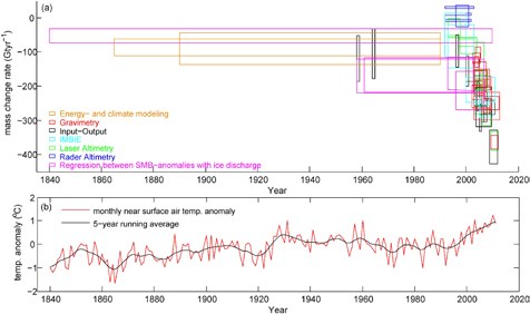
Figure 14. (a) Mass changes during 1840–2012. Colours refer to the different methods used to derive estimates. See table 1 for references. (b) The lower panel is the Greenland-wide near-surface air temperature anomaly updated from Box et al (2009). The solid red line denotes a 5 year running average.
Download figure:
Standard image High-resolution imageA number of recent efforts to model past atmospheric conditions over the GrIS, use output from long-term global atmospheric models as boundary conditions to force regional atmospheric circulation models. One suite of useful long-term global models is provided by the European Centre for Medium-Range Weather Forecasts (ECMWF) re-analysis project. The output from the global ECMWF re-analysis model covers September 1957–2002. There is also an updated ECMWF re-analysis Interim data set, which spans 1979 to the present. Thus, estimates of the GrIS mass balance that rely on ECMWF reanalysis data as input to determine the SMB of the ice sheet, extend back only to 1958.
Rignot et al (2008) provided a continual time series of the GrIS mass balance from 1958 onwards, that was based on an empirical relationship between 3 year-smoothed SMB-anomalies and ice discharge. They showed that during the 1960s the ice sheet was losing mass (at a rate of 110 ± 70 Gt yr−1), and that the ice sheet was in near balance during the 1970s and 1980s (30 ± 50 Gt yr−1); while from the 1990s and onwards the mass loss rate increased (1996: 97 ± 47 Gt yr−1; 2007: 267 ± 38 Gt yr−1), in accordance with other studies. Yang (2011) used an empirical melt sensitivity model to reconstruct the ice discharge, and arrived at a total mass loss rate of 170 ± 50 Gt yr−1 during 1958–2007 (see figure 14).
A longer record of mass balance change is provided by Box and Colgan (2013) who used ice core records and temperature reconstructions combined with regional climate model output to obtain a SMB time series from 1840 to the present. Using basically the same method as Rignot et al (2008), Box and Colgan (2013) generated a reconstruction of the mass balance which was scaled using independent GRACE observations (Box and Colgan also preferred parameterizing the ice discharge in terms of the 13 year smoothed runoff, rather than the 3 year smoothed SMB anomaly used by Rignot et al (2008). Box and Colgan (2013) found a total mass loss rate of 53 ± 21 Gt yr−1 during 1840–2010 (equivalent to a total sea level contribution of 2.5 ± 1.0 cm). Furthermore, their reconstruction showed considerable inter-decadal variability in the mass balance, yielding an ice sheet that was in near balance, even slightly positive, during the second half of the nineteenth century, while during the twentieth century their reconstruction revealed periods of considerable mass loss during 1920–mid-1930s, 1950–1970, and 2000–2010, and a positive mass balance during 1970–2000.
Alternative methods for estimating the mass balance change of the GrIS stem from sensitivity analysis to climate change and energy balance modelling. For example Zuo and Oerlemans (1997) modelled glacier mass balance sensitivity to climate change and historical temperature data and estimated a mass loss rate of 86 ± 25 Gt yr−1 (equivalent to a total sea level contribution of 2.7 ± 0.9 cm) during 1865–1990. This is consistent with van de Wal and Oerlemans (1994) who, based on calculations with an energy balance model, estimated a GrIS mass loss rate of 90 ± 47 Gt yr−1 (given in sea-level equivalents 2.5 ± 1.3 cm) between 1890 and 1990.
4. Sensitivity to external forcing
Mass loss from the GrIS is regionally distributed between sectors that exhibit different sensitivities to external forcing. Enhanced surface melting and speedup of glacier flow dominate the mass loss in the southeast, west, northwest and northeast parts of the GrIS, where most of the ice margin is in contact with the ocean. Here, the ice-ocean interface plays an important role, as warm oceans currents can significantly increase the melt rate at the glacier termini. Observations over the past two decades show that a speeding up of the many tidewater glaciers coincides with the entry of warmer waters into the fjord systems, enabling rapid retreat of the termini (Holland et al 2008, Murray et al 2010, Straneo et al 2010, 2012). Additionally, the rate of submarine melting is governed by the subglacial freshwater discharge (water that flows through channels at the glacier bed) from the grounding zone, as this drives the circulation of warm seawater that is brought into contact with the ice face through buoyancy-driven convection (Rignot et al 2010, Motyka et al 2011, Enderlin and Howat 2013). Furthermore, warmer water may reduce ice mélange in glacier fjords. Especially during winter, a reduction of ice in the fjord may result in higher than average-winter speed and lengthening of the duration of the high rate of iceberg production (calving) (Amundson et al 2010).
Both models and observations suggest that the speed up of, for example, Helheim, Kangerdlugssuaq, Jakobshavn, Upernavik, and Zachariae Isstrøm are responses to the retreat of the termini (Howat et al 2007, Price et al 2011, Khan et al 2013, 2014a, Nick et al 2013). The retreat reduces downstream resistive stresses, which are redistributed upstream. A bed that slopes down inland may lead to unstable grounding-line retreat, as increased flux and consequently reduced buttressing leads to thinning and eventual flotation of the glacier front, which makes the grounding line migrate inland into greater depths of the bed. Kangerdlugssuaq, Jakobshavn, and Zachariae Isstrøm possess a negative bed slope (Joughin et al 2012, Bamber 2013a, Khan et al 2014b) that lies below sea level, the key condition for satisfying the marine ice sheet instability hypothesis associated with parts of west Antarctica (Weertman 1974, Mercer 1978, Thomas 1979, Schoof 2007, Joughin et al 2014b). All three glaciers have retreated more than ~10 km during the last decade and continue to undergo dynamic thinning.
The shape of the outlet (i.e. bed elevation and width) is an important factor that can dominate glacier dynamics (Pfeffer 2007). A sensitivity study by Enderlin et al (2013) suggests that for glaciers with similar ice discharge, the trunks of wider glaciers and those grounded over deeper basal depressions tend to be closer to flotation, so that smaller amounts of dynamically induced thinning can result in rapid, unstable retreat following a perturbation. Therefore, glaciers that are subjected to similar external forcings may react quite differently. For example, Upernavik Isstrøm located in northwest Greenland consists of several outlets that retreated and thinned at different time intervals although they experienced the same external ocean and atmospheric forcings (Khan et al 2013). Additionally, the configuration of fjord bathymetry (e.g. the presence of sills and higher submerged plateaus) may have an effect on the exposure of the calving front to different layers in the water column (Andresen et al 2014).
The majority of the marine-terminating outlet glaciers in north Greenland are surrounded by year-round sea ice. Sea ice may resistive force that prevents the calving front from rotating and breaking off, reducing the calving rate and temporarily stabilizing the terminus (Amundson et al 2010, Nick et al 2012). Sea ice extent is typically maximum in March and minimum in September. In South Greenland, most coastal areas are free of sea ice between spring and autumn. However, fluctuation in sea ice concentration can have an effect on calving activities and flow speed near the terminus of a glacier. For example, the speed-up and breakup of Jakobshavn Isbræ's ice tongue in 1998 coincided with a period of reduced sea-ice concentration in nearby Diskobugten (Joughin et al 2008a). Similarly, Zachariae Isstrøm in north Greenland is surrounded by year-round sea ice. However, the breakup of Zachariae Isstrøm's ice tongue during 2002–2003 coincided with the absence of sea ice in the glacier fjord in September 2002 and 2003. Sea ice extent depends on, for example, atmospheric pressure, wind intensification, and air temperature. Over past decades, the number of storms and the air temperature in the arctic have increased, resulting in rapidly shrinking sea ice cover (Wang et al 2009, Screen et al 2011, Stroeve et al 2012).
Studies of the ice sheet's land-terminating glaciers (Zwally et al 2002, Bartholomew et al 2012, Palmer et al 2011, Sundal et al 2011) and marine terminating outlet glaciers (Joughin et al 2008b, Shepherd et al 2009, Andersen et al 2010) suggest that short-term speedups of ice flow are partially controlled by supraglacial streams and lakes that drain through moulins, and provide meltwater into subglacial environments that increases basal sliding. Though, a recent study by Schoof (2010) suggests that it is not simply the mean surface melt but the water input variability that is the main driver of short-term glacier velocity increases. Glacier sliding responds to melt indirectly through changes in basal water pressure.
Ice loss due to fluctuations in surface processes shows huge inter-annual and annual variability (van den Broeke et al 2009, Tedesco et al 2013). Over the last decade, melt and run off have significantly increased (van den Broeke et al 2009), resulting in a sustained increase of the ice mass loss rate. Melting records from 2010 and 2012 have especially shown that small fluctuations in, for example, the length of the melt season can more than double the SMB component of ice mass change, suggesting that both short- and long-term atmospheric forcing play an important role in the total mass budget. A study by Hanna et al (2014) suggests the recent years of warming are due to warm southerly winds over the western flank of the ice sheet, forming a 'heat dome' over Greenland and leading to the higher air temperatures. The above-normal, near-surface air temperatures observed during the 2010 melt record contribute to accelerated snowpack metamorphism and premature bare ice exposure, rapidly reducing the surface albedo (Tedesco et al 2011, Box et al 2012), resulting in widespread melting.
5. Recent advances in ice-sheet modelling
Glacier ice is a viscous non-Newtonian fluid—its flow is well-described by the Stokes equations known since the mid-nineteenth century. Challenges arise from specifying boundary conditions, especially at the ice sheet's interface with the lithosphere and the ocean (Vaughan and Arthern 2007).
Since the first thermomechanically-coupled ice sheet model was applied to the Greenland ice sheet in the late 1970s, numerical models have become important tools for studying the response of ice sheets to changes in environmental forcings. However, the inability of models constructed prior to 2007 to track observed rapid changes in Greenland's outlet glaciers, led the Intergovernmental Panel on Climate Change (IPCC) to exclude results from ice sheet models for their Forth Assessment Report (AR4) (IPCC 2007). This boosted model development, entailing significant improvements since AR4 was published.
First, early ice sheet models employed the 'shallow ice approximation' (Hutter 1983), that assumes flow is caused only by vertical gradients in shearing. Recent models implement a more complete representation of flow physics than the AR4 models. Most models now include horizontal stress gradients, though they differ in their treatment of longitudinal coupling. Hybrid models combine the shallow ice approximation for shearing in grounded ice, with the use of membrane stresses in ice shelves and areas of rapid sliding (Bueler and Brown 2009). Models in this category achieve a good compromise between accuracy and computational costs. Higher-order models (Blatter 1995) assume that pressure is determined by ice overburden pressure (the hydrostatic assumption) and ignore horizontal derivatives of the vertical velocity. Solving the Stokes equations without relying on simplifying assumptions is most accurate, but is computationally most demanding. Some ice sheet models can be configured with various stress-balance solvers (Larour et al 2012a, Brinkerhoff and Johnson 2013), allowing the choice of the most suitable approximation for the problem at hand. A novel approach that tries to balance computational efficiency with physical accuracy, is to vary the order of model complexity over the modelling domain (Seroussi et al 2012) such that the Stokes equations are only solved in areas where they are needed. Thanks to code parallelisation and advanced meshing techniques, century-scale prognostic simulations have become feasible using both higher-order (Brinkerhoff and Johnson 2013) and Stokes (Gillet-Chaulet et al 2012, Larour et al 2012a, Seddik et al 2012) models. However, longer integration times remain prohibitive due to large computational costs. Ice sheet models have also seen improvements in the way phase-changes are handled within temperate ice (i.e. ice at the pressure-melting point). Conventional temperature-based 'cold-ice' models are not energy conserving when temperate ice is present, as changes in the latent heat content in temperate ice are not reflected in the temperature state variable (Aschwanden et al 2012). Polythermal models, based on mixture theory, account for the latent heat content within temperate ice, thereby conserving energy. Among polythermal schemes, enthalpy-based formulations provide a unified treatment of conservation of energy for intra-, supra- and subglacial liquid water that is easy to implement into ice sheet models (Aschwanden et al 2012, Brinkerhoff and Johnson 2013, Seroussi et al 2013).
The predictive skill of a model, however, not only depends on model physics but also on the fidelity of the numerical implementation and the quality of data available for validation (Vaughan and Arthern 2007, Blatter et al 2011). Verification (i.e. the comparison of results from a numerical approximation to exact solutions of the same continuum model equations) has become an integral part of model development. A constantly-growing number of analytical solutions suitable for verification (Bueler et al 2005, 2007, Leng et al 2013, Bueler 2014) provides a partial alternative to hard-to-interpret intercomparison results (Bueler 2014), such as in Pattyn et al (2012). In engineering, validation is commonly defined as the process of comparing model results to a set of observations adequate to falsify a model (Roache 1998). Such validation is challenging to apply in ice sheet modelling; nonetheless attempts have been made (Robison et al 2010, Burton et al 2012). Direct validation of substantial sub-systems such as basal hydrology, thermodynamics, and ice dynamics is difficult or impossible as most or all observations available for validation are not linked to a single process, but are the consequence of a complex interplay between sub-systems. Alternatively, a model's predictive skill can be assessed, at least in part, by forcing a model with known or closely-estimated inputs for past events to see how well the output matches observations (hindcasting). For validation, spatially dense time series of observations are preferred metrics (Aschwanden et al 2013).
Second, a model is only as good as its initial conditions and time-dependent boundary forcing (Blatter et al 2011). In simple terms, the ice sheet model's task is to redistribute mass gain and loss at its upper and lower surfaces compatible with our understanding of ice sheet dynamics. Mass flux calculations are most sensitive to errors in ice thickness (or, equivalently, basal topography) (Larour et al 2012b), and it is the basal topography beneath the GrIS that controls the flow of ice and its discharge into the ocean (Morlighem et al 2014). While ice thickness data have been gathered from airborne radar echo soundings since the 1970s, data acquisition has been skyrocketing since 2009 thanks to NASA's mission Operation IceBridge, thereby vastly improving our picture of Greenland's basal topography, including the discovery of a mega canyon beneath the central GrIS (Bamber et al 2013b). To be useful for ice sheet models, sparse ice thickness measurements must be interpolated onto regular or irregular grids. Conventional geostatistical methods such as kriging (Bamber et al 2013a) lead to large errors in flux divergence (Morlighem et al 2013). This poses a fundamental limitation to ice sheet models, as unphysically large flux divergences force the ice sheet model to redistribute mass in order to reconcile topography and ice flow, and potentially converging to a steady state that is significantly different from the initial condition (Seroussi et al 2011). In fast flowing areas, errors in flux divergence can be greatly reduced by combining the sparse radar data with high-resolution flow measurements via mass conservation (MC; Morlighem et al 2013). An application of MC revealed deep submarine valleys aligned with fast flow features in Greenland (Morlighem et al 2014).
Next, Greenland's marine-terminating glaciers are sensitive, and respond rapidly, to oceanic perturbations (Howat et al 2007, Holland et al 2008, Nick et al 2009, Murray et al 2010). Processes in the vicinity of the ice sheet's interface with the ocean are complex, acting on a multitude of spatial and temporal scales, and (so far) prohibiting a unified theory. Numerical flow-line studies suggest that the thinning-induced change in basal effective pressure is the dominant process influencing near-terminus behaviour (Joughin et al 2012). Whole-ice-sheet models now show promise of being able to track the past two decades of observed outlet glacier changes (Price et al 2011). New theoretical work on calving, damage mechanics, and grounding line stability (Pralong and Funk 2005, Benn et al 2007, Schoof 2007, Amundson and Truffer 2010, Bassis 2011) is informing model development. Ice sheet models now implement first-order kinematic calving laws (Levermann et al 2012) as well as fracture/damage mechanics (Albrecht and Levermann 2012, Borstad et al 2012, Albrecht and Levermann 2014).
Finally, responding to the call for transparency in science and reproducibility of scientific findings (Nielsen 2011), open-source models are becoming increasingly popular. Ice sheet models capable of high-resolution, century-scale prognostic simulations that are open source include Elmer/Ice (Gagliardini et al 2013), the Ice Sheet System Model (ISSM; Larour et al 2012a), the Parallel Ice Sheet Model (PISM; www.psim-docs.org), and the Variational Glacier Simulator (VarGlas; Brinkerhoff and Johnson 2013).
5.1. Challenges and outlook
Boundary conditions such as the bed's stress and thermal state, are intrinsically difficult, if not impossible, to measure. Basal stresses, for example, can vary spatially and temporally by orders of magnitude and can depend strongly on local basal hydraulics, while measuring basal motion is difficult, expensive, and usually limited to a few isolated points (Greve and Blatter 2009). Despite decades of intensive research, no unifying theory of how basal stresses relate to basal motion is yet available. A high geothermal flux can locally raise the basal temperature to the pressure-dependent melting point, thereby initiating sliding. To make matters worse, heat flow is heterogeneous and can vary on scales of less than 100 km (Dahl-Jensen et al 2003, Näslund et al 2005). So far, few direct measurements of heat flux exist (Fahnestock et al 2001), and indirect methods (Shapiro and Ritzwoller 2004, Fox Maule et al 2005) have limited accuracy (Alley and Joughin 2012). While the exponential dependence of ice viscosity on temperature is reasonably well-constrained by measurements, high shear rates near the bed result in strongly anisotropic flow characteristics. At the pressure melting point, additional ice softening occurs due to the presence of liquid water (Duval 1977), though this relationship remains poorly quantified (Duval 1977, Lliboutry and Duval 1985).
It has become evident that variations in surface melting affect not only the flow speed of mountain glaciers (Iken 1978, 1981), but also near-coastal areas of the GrIS (Zwally et al 2002, Das et al 2008, Palmer et al 2011). The impact of these fluctuations on the GrIS in a warming climate has not yet been quantified (Sundal et al 2011). Recent theoretical and numerical studies (Schoof 2010, Hewitt 2011, Werder et al 2013, de Fleurian et al 2014) on idealised geometries and mountain glaciers are guiding the development of numerical subglacial hydrology models applicable to the GrIS (Bueler and Pelt 2014). However, any such model has a necessarily large number of parameters for which none or few observational constraints yet exist, making comprehensive parameter sensitivity studies indispensable. In addition, basal hydrology models are computationally expensive because water movement in the subglacial aquifer is fast compared to the flow of the overlying ice, and numerical schemes must choose small time steps accordingly.
As observations alone are insufficient to provide the initial conditions for prognostic ice sheet models, data assimilation techniques must be combined with parameterisations of processes to provide the necessary initial and boundary conditions. Reconstruction of basal properties using inverse methods has become an integral part of ice sheet modelling. High-resolution surface velocity is the most commonly used observable in the assimilation process, but recent work by Larour et al (2014) also includes time-dependent surface altimetry data. Remaining inconsistencies in initial conditions cause large flux divergences that result in transient signals propagating through the system at the beginning of the run (Gillet-Chaulet et al 2012, Brinkerhoff and Johnson 2013). Also, the parameter fields resulting from inversion may not be applicable for prognostic simulations, as these parameters evolve with time (Aschwanden et al 2013). Ideally, inverse methods are applied to recover material properties, such as till friction angle, and the connection to time-evolving basal drag should be made by subglacial hydrology models. Initialising ice sheet models is challenging; the initial state needs to be close to the currently-observed ice sheet, including the temperature field, while at the same time remaining fully self-consistent with climate forcing in order to minimise unnatural transients in the model response, but also maintain the natural response of the model which results from its initial state (Aðdalgeirsdóttir et al 2014).
Model simulations prepared for the Fifth Assessment Report (Vaughan 2013) of the IPCC suggest that over the next two centuries the evolution of the GrIS will most likely be dominated by uncertainties in future SMB (Bindschadler et al 2013, Nowicki et al 2013), though the recently discovered presence of deep, widespread submarine glacial valleys around Greenland implies that Greenland outlet glaciers remain the wild card (Morlighem et al 2014). Accurate modelling of SMB relies on realistic simulation of local climate, snow processes, albedo evolution, refreezing, and adequate horizontal resolution to capture high SMB gradients at ice sheet margins (Vizcaíno 2014). To capture the SMB elevation feedback, ice sheet models need to be directly coupled to general or regional circulation models. A core requirement of successful two-way coupling is the conservative exchange of mass and energy fluxes between the models (Fischer et al 2014). The first realistic results of fully-coupled models are now emerging (Vizcaíno et al 2013, 2014, Fyke et al 2014). Alternatively, parameterisations of SMB changes have been proposed (Helsen et al 2012, Franco et al 2012, Edwards et al 2014a) and tested (Edwards et al 2014b).
Substantial challenges also remain where the ice is in contact with the ocean. Furthering our understanding of ocean-induced ice sheet melting is currently hampered by the logistical difficulties of observational studies (Joughin et al 2012), and the early developmental state of coupled high-resolution, ocean-ice sheet models.
6. Concluding remarks
Mass loss from the GrIS is a complex function of processes related to SMB and ice dynamics, forced mainly by short- and long-term fluctuations in the atmospheric and oceanic energy input. Measurements from combining satellite altimetry, airborne altimetry, interferometry, and gravimetry data sets over the last decade show a doubling of the ice loss rate due to a combination of increased ice discharge and SMB-inferred mass change (Pritchard et al 2009, van den Broeke et al 2009, Moon et al 2012). Khan et al (2014), for example, obtained an ice loss rate of 172.4 ± 21.7 Gt yr−1 during 2003–2006 and 359.8 ± 28.9 during 2009–2012. However, the trend from 2003–2012 was 274 ± 24 Gt yr−1 (see table 1), with an approximately equal split between surface processes and ice dynamics. Studies using airborne laser altimetry, satellite radar altimetry, and the input–output method suggest a much lower mass loss rate of 50–100 Gt yr−1 in the 90s (see table 1). Extending the record back to 1840 suggests a long-term mass loss rate of 50–90 Gt yr−1 over the last century (see figure 14). During the twentieth century the rate of mass change was highly variable with a much higher mass loss rate during the warming in the 1920s and 1930s, while the ice sheet was near balance during the 1970s and 1980s (Rignot et al 2008, Box and Colgan 2013). The variability is also clear from historical aerial images combined with both early and modern satellite imagery covering outlet glaciers. These data sets allow long-term mapping of the glacier front positions, and thus permit indirect evaluations of ice discharge. From extensive spatial coverage, it is also clear that different outlet glaciers can react differently to comparable external atmospheric and oceanic forcings. This suggests that other factors, such as the shape of the glacier outlet and the fjord bathymetry, are important components for determining the short- and long-term behaviour of the glaciers.
One of the major questions regarding the future stability of the GrIS, is whether the mass loss will continue to accelerate as air and ocean temperatures increase. Recent mapping of the subglacial topography (Morlighem et al 2014) has shown Greenland to possess much larger deep, incised, subglacial fjords than previously thought. Those features are believed to amplify the acceleration of ice discharge.
Ice sheet modelling has come a long way since the publication of AR4, and even more so since the first application of an ice sheet model to the GrIS. Ice sheet models have seen key improvements in the way they handle stresses and the thermal state within the ice. Better representation of marginal processes and increased grid resolution is facilitating the tracking of changes in outlet glaciers and their marine termini. However, no ice sheet model has demonstrated sufficient skill in hindcasting the evolution of the Greenland ice sheet during the past decades; until then model-based century-scale sea-level projections should be taken with a grain of salt. Some of the issues, while being far from trivial, are no road blocks on the path to progress. Within a decade model coupling techniques will mature sufficiently for ice sheets to become a standard part of Earth System Models, capturing feedbacks between all the physical systems involved. Thanks to the ever-increasing availability of high-performance computing systems, fully-coupled simulations will be feasible at grid resolutions sufficient to resolve the high gradients in surface mass balance and the changes in fast flow in outlet glaciers. Model coupling must be complemented by innovative approaches to model initialization. Targeted observations, especially at the lateral and basal boundary, will reduce uncertainties in boundary conditions, provide valuable input for model validation, and further our process understanding. These observations will also help answering whether Stokes models are warranted or computationally-efficient lower-order approximations are sufficiently accurate for sea-level predictions. As suggested by Vaughan and Arthern (2007), we will perform ice sheet forecasts similarly to weather forecasts where suites of models are continuously run with different initial conditions. These efforts are to be accompanied by rigorous formal sensitivity analyses to assess uncertainty propagation. Furthermore we will quantify the time scale when ice sheet weather turns into ice sheet climate. Despite all anticipated progress, major obstacles in the quest for better sea-level predictions are, and will remain, our limited understanding of the physical processes at the ice-ocean interface and the lack of a prognostic sliding law. The challenges here are multifold. First, measurements where the ice meets the ocean are inherently difficult and the bottom of an ice sheet will remain largely inaccessible. Next, it is unclear if the currently-observed quantities are sufficient to characterise the physical processes we are trying to understand. Are there quantities we could measure additionally that would facilitate progress? Last, we must cast our process understanding into a set of equations that can be solved numerically. A 'grand string theory' of glaciology spanning across temporal and spatial scales is unlikely to emerge in the next decade; instead smaller and larger pieces will have to be laboriously put together like a jigsaw puzzle. Of course good things don't come easy, and all good things take some time. Substantial progress can only arise from a concerted community effort in which ice sheet modellers have become well-integrated within the broader climate modelling community.

Figure 15. Illustration of advances in ice sheet modelling since AR4 (IPCC 2007). (a) and (d) Observed surface speeds from Joughin et al (2010).(b) and (e) A model simulation using model physics and forcings available prior to AR4. (c) and (f) A model simulation using model physics and forcings available in 2014. It is important to note that this simulation did not use observed surface velocities during data assimilation. (a), (b) and (c) show zoom over Jakobshavn Isbræ.
Download figure:
Standard image High-resolution image