Abstract
I overview new aspects of the structure of exotic nuclei as compared to stable nuclei, focusing on several characteristic effects of nuclear forces. The shell structure of nuclei has been proposed by Mayer and Jensen, and has been considered to be kept valid basically for all nuclei, with well-known magic numbers, 2, 8, 20, 28, 50, .... Nuclear forces were shown, very recently, to change this paradigm. It will be presented that the evolution of shell structure occurs in various ways as more neutrons and/or protons are added, and I will present basic points of this shell evolution in terms of the monopole interaction of nuclear forces. I will discuss three types of nuclear forces. The first one is the tensor force. The tensor force is one of the most fundamental nuclear forces, but its first-order effect on the shell structure has been clarified only recently in studies on exotic nuclei. The tensor force can change the spin–orbit splitting depending on the occupation of specific orbits. This results in changes of the shell structure in many nuclei, and consequently some of Mayer–Jensen's magic numbers are lost and new ones emerge, in certain nuclei. This mechanism can be understood in an intuitive way, meaning that the effect is general and robust. The second type of nuclear forces is central force. I will show a general but unknown property of the central force in the shell-model Hamiltonian that can describe nuclear properties in a good agreement with experiment. I will then demonstrate how it can be incorporated into a simple model of the central force, and will discuss how this force works in the shell evolution. Actually, by combining this central force with the tensor force, one can understand and foresee how the same proton–neutron interaction drives the shell evolution, for examples such as Sn/Sb isotopes, N = 20 nuclei and Ni/Cu isotopes. The distribution of single-particle strength is discussed also in comparison to (e,e'p) experiment on 48Ca. The shell evolution affects shapes of nuclei through Jahn–Teller-type mechanism, and a very interesting example with exotic Si isotopes is discussed. The third type of nuclear force is a three-body force, which originates in the Δ particle excitation as proposed by Fujita and Miyazawa many years ago. This force is shown to produce a repulsive interaction between valence neutrons after averaging effects from the third nucleon in the core. The same three-body force is responsible for neutron stars. By including such effects of the three-body force, one can predict the correct drip line of oxygen isotopes, for instance. Thus, the landscape of atomic nuclei varies in going from stable to exotic nuclei due to particular nuclear forces, leading to a paradigm shift. This paper overviews some basic ideas and selected examples.
Export citation and abstract BibTeX RIS
1. Introduction
The landscape of atomic nuclei has been and is still being changed significantly during the last two decades. This is primarily because the frontier of nuclear structure physics has moved forward from stable nuclei to exotic ones. Here, stable nuclei mean the atomic nuclei with infinite or sufficiently long life times, while exotic nuclei stand for the atomic nuclei with shorter life times and are characterized, in most cases, by unbalanced ratio between the proton number (Z) and the neutron number (N).
Some paradigms have been working in the study of the structure of atomic nuclei over many decades, and there seems to be a belief that those paradigms hold for basically all nuclei, even for those not yet observed. This belief had not been doubted seriously, partly because there had been no experimental symptoms against it. The situation has begun to change since the end of the last century, however. In fact, the belief is being challenged by recent developments of nuclear structure physics with certain hints of paradigm shifts. This paper is devoted to one of such developments.
The first step of such developments was made by the experiment measuring the radius of the 11Li nucleus by Tanihata et al in 1985 using RI (radioactive ion or rare isotope) beams of this nucleus. This experiment indicated that 11Li shows extraordinarily large interaction cross section [1]. This exciting result has been interpreted in terms of neutron halo by Hansen and Jonson in 1987 [2]. Here, the neutron halo implies extremely extended radial wave function of loosely-bound neutrons due to their tunneling effect.
The appearance of the neutron halo can be understood naturally with the nuclear chart. In fact, figure 1 shows a left-lower part of the nuclear chart where individual nucleus is indicated by a box located at its Z and N. It starts from one neutron (Z = 0, N = 1), which is indeed the simplest nucleus with finite life time (half life ∼ 10 min). Stable nuclei are shown by blue boxes in figure 1. The lightest stable nucleus is a proton, which is nothing but the nucleus 1H with Z = 1 and N = 0. The deuteron is also a stable nucleus (Z = N = 1). Stepping over helium (Z = 2) isotopes, one comes to lithium isotopes (Z = 3). Two isotopes 6,7Li are stable. By adding neutrons, one can create 8,9Li, which are bound by the nuclear force (strong interaction) but decay by β-process with short life time. In going to heavier isotopes with a fixed Z but larger values of N, Fermi energy of neutrons goes up, and the binding energies of last neutrons become smaller. In the case of Li isotopes, the nuclear force cannot bind the last neutron in 10Li. However, in 11Li, we have two last neutrons, for which the binding from 9Li is not enough but these two neutrons attract each other, resulting in bound 11Li nucleus. Although the binding energy is very small, this nucleus is definitely bound by nuclear force, and its decay is through a β-process. Such a tiny binding energy results in loose binding of these two neutrons, leading to their wave functions extended very far due to tunneling effect as pointed out by Hansen and Jonson [2]. The radius of 11Li is, in fact, as large as that of a much heavier nucleus 208Pb. Here the argument looks very natural and straightforward, but a certain time passed before this idea was widely accepted. There were several other interpretations, for instance, large deformation.

Figure 1. Left-lower part of the nuclear chart. A nucleus is expressed by a box located at its neutron number (N) and proton number (Z). Blue squares imply stable nuclei. Exotic nuclei confirmed experimentally are shown by yellow squares, while green square denote those with neutron halo. The year of discovery of most neutron-rich isotope is shown at far right as well as the name of the element. Modified from figure 1 of [3] which is based on [4]. 8Be and 9B are not included as (bound) exotic nuclei because the nuclear force cannot keep them bound.
Download figure:
Standard imageExperimental hunting for other nuclei with the neutron halo has been conducted in several laboratories with RI-beam capabilities. So far, some nine nuclei have been known to exhibit neutron halo as shown in figure 1. Exotic nuclei have their existence limit beyond which no more neutrons can be added. This limit is called the neutron drip line collectively. (There is a proton drip line as well, but we do not discuss it in this paper.) The neutron halo is naturally a characteristic feature of exotic nuclei near or on the drip line. The neutron halo is certainly one of the greatest advancements of nuclear physics made by RI-beam technology. It has been and still is a subject of great interest experimentally and theoretically, as discussed also in this symposium. We, however, focus on another major development with exotic nuclei, as we shall now turn to.
In figure 1, stable nuclei (blue square) form an object like a thin line on the nuclear chart. Although this is not a perfectly continuous line, this set of stable nuclei is called the (β) stability line.
The neutron drip line has been established up to oxygen isotopes (Z = 8). Beyond Z = 8, the neutron drip line is not presently known, and should be further away from the rightmost isotopes in figure 1. While 11Li is four units of N away from the stability line, as the proton number Z becomes larger (going up in the nuclear chart), the distance between the stability line and the drip line on the nuclear chart becomes longer. For instance, one finds, in figure 1, that 13 isotopes have already been known for Mg (Z = 12) besides stable ones. The number of such isotopes keeps becoming more and more as Z increases. These nuclei are all bound, and most of them are even well bound as we shall see later. A question, which occurred to me at the end of the last century, is whether or not there could be new physics in those nuclei. This question must be independent of the loose binding phenomena, but should be related definitely to nuclear forces which may work in different manners as compared to stable nuclei.
I would like to discuss, in this paper, how such a question led to some new findings and perspectives of nuclear structure. I would like to focus on basic ideas, concepts and pictures rather than detailed descriptions.
We begin by looking at the whole nuclear chart as shown in figure 2. One immediately finds that the distance between the stability line and the drip line keeps expanding as Z becomes higher. Figure 3 presents the number of bound nuclei including theoretically predicted ones, as a function of Z. We can see that this number becomes very large, as large as more than 50 for Z ⩾ 70. If there are so many new objects, it is natural to expect some qualitatively new phenomena and/or mechanisms.

Figure 2. Nuclear chart based on [5]. Each nucleus is expressed by a box with the neutron number (N) and the proton number (Z). Blue squares imply stable nuclei. Exotic nuclei observed experimentally are shown by brown squares, while green square denote those predicted only. Dark green arrows indicate the path of the r process schematically. Courtesy of T Yoshida and N Shimizu.
Download figure:
Standard image
Figure 3. The number of bound isotopes including exotic ones as a function of the proton number Z based on [5]. The number of those with small two-neutron separation energy (⩽2 MeV) are distinguished by dark blue. Courtesy of N Shimizu.
Download figure:
Standard image2. Shell structure, magic numbers and monopole interaction
The nuclear shell model was started by Mayer and Jensen more than 60 years ago by identifying the magic numbers and their origin [6]. The study of nuclear structure has been advanced on the basis of the shell structure associated with those magic numbers. Such studies, on the other hand, have been made predominantly for stable nuclei and their neighbors on the nuclear chart. In fact, only these nuclei have been accessible experimentally for many decades, except for a few cases. In such stable nuclei, the magic numbers suggested by Mayer and Jensen remain valid, and the shell structure can be understood well in terms of the harmonic oscillator potential with a spin–orbit splitting.
The harmonic oscillator potential can be understood by combining (i) nearly constant nucleon density inside the nucleus (density saturation) and (ii) short-range attraction from nuclear forces. For more detail, if one looks at a nucleon (called x for convenience) inside a nucleus, there should be an approximately constant number of nucleons within the range of nuclear forces. This means that the effect of the nuclear force does not depend on the location of the nucleon x, if it is well inside the nucleus. We thus obtain rather flat mean potential inside the nucleus. If the location of the nucleon x is near the surface of the nucleus, the number of nucleons interacting with the nucleon x through the nuclear force becomes smaller, leading to shallower potential. If the nucleon x is far from the nuclear surface, the mean potential is vanished. This intuitive consideration leads us to a Woods–Saxon potential, which can be further approximated by a harmonic oscillator potential inside and near the surface of the nucleus. The difference well outside the surface does not matter, because the wave functions of bound nucleons are not stretched out there with sizable amplitudes.
By adding the spin–orbit splitting, we end up with the harmonic oscillator potential + spin–orbit model as Mayer and Jensen did in 1949 [6] (Nobel Prize in Physics for their work on the shell model in 1963). As this picture looks sound and robust, it seems impossible to find a way out of this picture. However, there are some factors which are not included in the mechanism of Mayer and Jensen. Those factors are related more directly to nuclear forces, and I shall discuss them in this paper.
The effects of nuclear forces on the shell structure can be studied in terms of monopole component or interaction of a given two-body interaction,  . We first define the monopole matrix element of an interaction,
  , as
, as
where j and j' denote single-particle orbits with k and k' being their magnetic substate, respectively, and  is the antisymmetrized two-body matrix element. Equation (1) implies an averaging over all possible orientations of two interacting particles in the orbits j and j', while the antisymmetrization (Pauli principle) is taken into account.
The monopole component of  is written, for j ≠ j', as

where  (
( ) is the number operator of orbit j (j').1 The monopole interaction, denoted
  , is defined as the operator consisting of
  for all possible pairs of j and j' for j ≠ j' and slightly more complicated terms for all pairs of j = j' (see footnote 1).
As we mentioned, the monopole component of the interaction  is nothing but the average of effects of
  , and it depends only on the number operators of these orbits. Its initial idea was introduced by Bansal and French [7], while its relevance to the effective shell-model interaction was discussed by Poves and Zuker [8].
Note that the monopole interaction  can be defined either in the isospin formalism where the monopole interaction has the index T = 0 and 1 with slight modification, or in the proton–neutron scheme, e.g. nj for proton and nj' for neutron. In some cases, 'j,j'' may be omitted for brevity.
The importance of the monopole interaction for exotic nuclei originates in its linearity. As the orbit j' is occupied, the single-particle energy (SPE),  j, of an orbit j is shifted by (see footnote 1),

For j' = g9/2 as an example, nj' takes values up to 10, and a typical monopole matrix element, 0.1 MeV, yields a change of SPE, Δj, up to 1 MeV. Thus, the effect of the monopole component can be magnified considerably in many cases. By moving along the nuclear chart, one can indeed change a particular nj' substantially. This highlights the physics of exotic nuclei compared to that of stable nuclei.
Another important point with the monopole interaction is its trace-type nature, as is clear from the summation in equation (1). Because of this, at shell closures, the monopole component produces effects according to equation (3) with the values of nj' corresponding to the full occupation of the valence shell. In contrast, effects of the other (i.e., multipole) components of  vanish, as they are of traceless character. Namely, only monopole component survives when a closed shell is formed, whereas the other multipole components yield vanished effects. Thus, the monopole component governs also (spherical) SPEs at shell closures. In open shell systems, its effects can be viewed through equation (3) as effective SPEs (ESPEs). Note that such effects are included automatically in the diagonalization of the shell-model Hamiltonian, because the monopole component is a part of the Hamiltonian. By the monopole interaction, we can foresee or interpret what happens in a shell-model calculation, without performing the diagonalization of the Hamiltonian which is not a trivial task in many cases. As the surface deformation with low excitation energies is a Jahn–Teller effect, the SPEs (and ESPEs) should play crucial roles for collectivity in many cases.
The two-body interaction in the shell model is often referred to as 'residual interaction' as compared to mean potential. This characterization may be reasonable to multipole components, whereas it may not be so appropriate to the monopole component which produces linear effects and becomes a part of the mean potential at the shell closure.
3. Spin–isospin interaction and shell evolution
The changes of the shell structure, called shell evolution hereafter, in exotic nuclei due to nuclear forces was discussed for the first time in 2001 in [9]. The change due to loose binding was discussed before that time, but the change of the shell structure, independent of loose binding, had not been discussed in a systematic way.
Figures 4(a) and (b), reprinted from [9], show the shell evolution between 30Si (stable nucleus) and 24O (exotic nucleus). In the filling scheme, six protons occupy 0d5/2 orbits in 30Si, whereas no proton is there in 24O. In this calculation, the SDPF-M shell-model Hamiltonian [10] is used, of which the monopole interaction between proton 0d5/2 and neutron 0d3/2 is strongly attractive, and produces the change between figures 4(a) and (b), following the rule in equation (3). The SDPF-M Hamiltonian is quite reasonable and very successful with respect to the agreement with experiment. It was therefore amazing that the shell structure changes to such an extent that the magic number moves from N = 20 to 16 [9].

Figure 4. Neutron ESPE's for (a) 30Si and (b) 24O, relative to 1s1/2. The dotted line connecting (a) and (b) is drawn to indicate the change of the 0d3/2 level as an example of the shell evolution. (c) The major interaction producing the basic change between (a) and (b). (d) The process relevant to the interaction in (c). Reprinted from figure 1 of [9]. Copyright (2001) by the American Physical Society.
Download figure:
Standard imageThe under-lying origin of such a change was discussed in [9]. It was conceived that the driving force should be a spin–isospin interaction because of the selectively strong coupling between proton 0d5/2 and neutron 0d3/2. A simple spin–isospin interaction was considered, which was a central force with spin dependence

where  (
( ) denotes the isospin (spin) of nucleons 1 and 2, and the symbol ( · ) means a scalar product. Here, c(r) is a function of the relative distance, r. For the long range limit of the central force, analytic expression was derived for its monopole matrix elements (see table I of [11] also).
Further studies clarified, however, that this interpretation is not the right one, while the monopole component of the shell-model interaction is still adequate. The correct understanding of figure 4 has been known, by now, to be obtained by replacing the spin-dependent central force in figure 4(d) with tensor force, another but predominant spin–isospin interaction. Thus, although the idea of strong monopole interaction and resultant shell evolution proposed in [9] played a crucial role as the initial step towards more comprehensive understanding, we had to wait until 2005 for a more complete picture, when the shell evolution by the tensor force was presented. Let us move on to this subject.
4. Tensor force and shell evolution
In the shell-structure scheme of Mayer and Jensen proposed in 1949 [6], one of the missing elements is the first-order contribution of the tensor force. Shell-model interaction or effective interaction in low-momentum space contains strong renormalization effects on its central-force component from multiple actions of the tensor force. In fact, pion exchange primarily generates the tensor force, and multiple exchanges of pions provide us with the strong central force. Much of nuclear binding is due to this central force [12].
Besides such effects, the tensor force produces another very important and intriguing effect in its lowest order, or, by one-pion exchange process. This effect must have been contained in numerical results, but its simple, robust and general features have not been mentioned or discussed until the work done in [13], where the change of the shell structure, called the shell evolution, due to the tensor force was presented for the first time.
The tensor force due to one-pion exchange is written as

where [ ](K) means the coupling of two operators in the brackets to an angular momentum (or rank) K, and Y denotes the spherical harmonics for the Euler angles of the relative coordinate. Here, f(r) is a function of the relative distance, r. Equation (5) is equivalent to the usual expression containing the S12 function. Because the spins  and
and  are dipole operators and are coupled to rank 2, the total spin S (
 ) of two interacting nucleons must be S = 1. This plays a crucial role in the shell evolution by the tensor force as pointed out later. If both of the bra and ket states of VT have L = 0, with L being the relative orbital angular momentum, their matrix element vanishes because of the Y(2) coupling. These properties are used later also.
We begin with cases like figure 5: with orbital angular momenta being denoted by l or l', protons are in either j> = l + 1/2 or j< = l − 1/2, while neutrons are in either j'> = l' + 1/2 or j'< = l' − 1/2. In examples to be discussed, these orbits represent valence or hole states near Fermi surface, and their radial wave functions are given by the harmonic oscillator potential for simplicity. From now on in this section, V stands for the tensor force.

Figure 5. (a) Schematic picture of the monopole interaction produced by the tensor force between a proton in j>,< = l ± 1/2 and a neutron in j'>,< = l' ± 1/2. (b) Exchange processes contributing to the monopole interaction of the tensor force. Reprinted from figure 1 of [13]. Copyright (2005) by the American Physical Society.
Download figure:
Standard imageThe question is as to how the tensor force drives ESPEs, and whether there is a general rule for this change. The answer is given in an intuitive way first. Figure 6(a) depicts the case that a nucleon on j< is interacting with another on j'> through the tensor force. The total spin must be S = 1. We assume that the total spin is up, and therefore the spin of each nucleon is also up. The orbital motion of two nucleons then should be opposite as shown in figure 6(a). We discuss the relative motion of the two interacting nucleons, as the interaction between them is relevant only to their relative motion but not to their center-of-mass motion. We model the relative motion by linear motion on the x-axis of two free nucleons (i.e. plane waves). This modeling is reasonable for the interaction with the range shorter than the scale of the orbital motion, which should be the case now. In figure 6(a), this means that the motion in the yellow-colored region, 'wave function of relative motion', is described as a linear motion on the x-axis being the horizontal direction on the plane of this paper. Clearly the two nucleons are coming from the opposite directions on the x-axis. We assign indexes 1 and 2 to the two nucleons. Their wave numbers are k1 and k2, while their coordinates are denoted by x1 and x2. The wave function, Ψ, consists of products of two plane waves. We take a system of a proton and a neutron in total isospin T = 0. The antisymmetrization is imposed. Because of S = 1, the coordinate wave function must be symmetric as,

where center-of-mass and relative momenta are defined, respectively, as,

and center-of-mass and relative coordinates are likewise as,

From these equations, we see that the relative motion is expressed by the wave function

and the center-of-mass motion has a wave number K.

Figure 6. Intuitive picture of the tensor force acting two nucleons on orbits j and j'. Reprinted from figure 2 of [13]. Copyright (2005) by the American Physical Society.
Download figure:
Standard imageIn the case of figure 6(a), assuming k1 ∼ − k2, we obtain K ∼ 0, the center-of-mass being almost at rest, meaning a nearly uniform wave function of the center-of-mass motion. On the other hand, the relative motion has a large momentum, k ∼ 2 k1. Based on Fermi momentum in nuclei, k is considered to be of the order of magnitude 1 fm−1, but not to exceed ∼1.5 fm−1. From the range of the force, the area inside x ∼ 1 fm is relevant. Thus, the relevant region of kx in equation (9) is within |kx| ∼ π/2. The wave function in equation (9) is damped more quickly with |x| in this region for k larger. Because of this damping, the wave function of the relative motion relevant to the effects of the tensor force is suppressed on the x-axis. We now come back from one-dimensional modeling to the orbital motion. A similar damping of the relative-motion wave function occurs as shown by the yellow area in figure 6(a), implying that the relevant part of the wave function has a shape suppressed in the direction of the orbital motion, or equivalently stretched in the direction of the total spin. This is similar to the deuteron, and we obtain attractive effect from the tensor force robustly.
In the case of figure 6(b), the center-of-mass moves fast with K large. On the other hand, k ∼ 0 is obtained, implying a stretched wave function of the relative motion on the x-axis. In this case, the two nucleons are more apart from each other in the direction perpendicular to the total spin, as indicated by the yellow area in figure 6(b). The tensor force then produces a repulsive effect.
Thus, we obtain a robust picture that j< and j'> (or vice versa) orbits attract each other, whereas j> and j'> (or j< and j'<) repel each other. Note that the essence of the above one-dimensional explanation can be understood in terms of Heisenberg's uncertainty principle.
The coordinate wave function is symmetric in the above argument, corresponding to the coupling between S and D waves of the relative motion. If the total isospin is T = 1, the antisymmetric coordinate wave function is taken, corresponding to P waves. In this case, the wave function in equation (9) is replaced by sin(kx). This wave function produces a horizontally stretched wave function, reversing the above argument for the case in figure 6(a). However, because of the isospin dependence, there is another sign change, producing an attractive effect totally. Thus, j>–j'< and j<–j'> couplings always give us an attractive effect, whereas j>–j'> and j<–j'< couplings are repulsive.
The radial wave functions of the two orbits must be similar in order to have a large overlap in the radial direction. A narrow spacial distribution is favored in the radial direction, in order to have a 'deuteron-like' shape. This is fulfilled if the two orbits are both near the Fermi energy, because their radial wave functions have rather sharp peaks around the surface. If the radial distributions of the two orbits differ, not only the overlap becomes smaller but also the relative spacial wave function is stretched in the radial direction, which is against the deuteron-like shape, making the effect less pronounced. Note that for the same radial condition, larger l and l' enhance the tensor monopole effect in general, as their relative momentum becomes higher (see figure 6).
We have presented the intuitive explanation of the shell evolution due to the tensor force. An identity on the monopole interaction of the tensor force has been derived in [13], showing a consistent result in a mathematical and rigorous way. Namely, for the orbits j and j', the following identity has been derived for the tensor force in [13],

where T = 0 and 1, and j' is either j'> or j'<. Note that this identity is in the isospin formalism, and can be applied not only to cases like figure 5(a) but also to cases between neutrons or between protons. The identity in equation (10) can be proved by angular momentum algebra by summing all spin and orbital magnetic substates for the given l. It is assumed that the radial wave function is the same for j> and j< orbits, which is exactly fulfilled in the harmonic oscillator and practically so in other models if the orbits are well bound. This identity does not hold if the single-particle state j> or j< is identical to j' (as excluded in figure 5), because the substate summation is affected by the isospin symmetry. However, the actual monopole matrix elements follow the relation in equation (10) semi-quantitatively. One can prove that VT j, j' = 0 for j or j' = s1/2. Equation (10) suggests that if both j> and j< orbits are fully occupied, their total tensor monopole effect vanishes.
Only exchange processes in figure 5(b) contribute to VM for the tensor force, while its direct contribution vanishes. The same property holds for a spin–spin central interaction [9]. If only exchange terms remain, the spin-coordinate part of the T = 0 and 1 matrix elements are just opposite. Combining this with  in equation (5), one obtains

Thus, the proton–neutron tensor monopole interaction is twice as strong as the T = 1 interaction.
The tensor force is due to pion (π) exchange, but the rho meson (ρ) contributes also. In the following, we use the π + ρ meson exchange potential [13]. The coupling constants are taken from [14].
Here we present an example as to how the shell evolution occurs due to the tensor force. This example is for the splitting between proton 0h11/2 and 0g7/2 orbits on top of Sn isotopes with changing neutron number. The strength distribution of these single-particle states have been measured for some Sb (Z = 51) isotopes by transfer reactions [15]. Figure 7 shows a comparison between theoretical results and experimental ones. The theoretical calculations have been performed by two methods: (i) with central and tensor forces, and (ii) with central forces only. We used the central force to be explained in the next section. The calculation was done for the changes of (effective) SPE. We take the experimental energies at N = 64 as the origin, and see the changes from there. As the neutron number increases, the proton 0h11/2 and 0g7/2 orbits start to repel each other. The calculation only with the central force keeps this 0h11/2–0g7/2 gap unchanged or even reduces it. On the other hand, once the tensor force is included, the repulsion between 0h11/2 and 0g7/2 orbits is obtained quite well without any adjustment. This is the first example indicating the shell evolution due to the tensor force. We shall come back to this in the next section.

Figure 7. SPEs of proton 0h11/2 and 0g7/2 orbits on top of Sn isotopes as functions of the neutron number N. The solid lines are calculations with the tensor-force effect, whereas the dotted lines are without it. Symbols are experimental data: fragmentation of single-particle strength is considered for filled circles, while bare levels are used for open symbols. Experimental data are from Schiffer et al [15].
Download figure:
Standard image5. Shell evolution due to the central and tensor forces
We analyze, in this section, the monopole interaction of major shell-model interactions that describe experimental data very well, making anatomy of it in terms of central and tensor forces.
Figure 8(a) shows vm; j, j' for isospin T = 0 from the GXPF1A interaction, the G-matrix interaction [17, 18] and the tensor force in the pf-shell. The tensor force refers, as already mentioned, to the π + ρ meson exchange force. The orbits (j,j') are grouped as (f, f), (p, p) and (f, p). In figure 8(a), we find two distinct kinks in the tensor-force values for the (f, f) and the (p, p) groups, and the same kinks appear also in the GXPF1A and the G-matrix results. Note that each kink is a consequence of the general rule suggested in the previous section with figure 6. The similarities are remarkable. To shed more light on this, in figure 8(b) we subtract the tensor-force contribution from the GXPF1A and the G-matrix values. This results in almost flat curves. The (f, f) and (p, p) cases show almost the same values, while the (f, p) shows higher (i.e., small absolute magnitude) but still nearly flat values. This can be understood in terms of radial integral of the central force: in the former case the radial wave functions are the same between j and j', while they are different in the latter. The flatness suggests a longer-range central force. In order to incorporate these features, we introduce a central Gaussian interaction as

where S(T) means spin (isospin), P denotes the projection operator onto the channels (S,T), and f, r and μ stand for the strength, internucleon distance and Gaussian parameter, respectively. Figure 8(b) shows results obtained by f0,0 = f1,0 = 166 MeV and μ = 1.0 fm. The agreement with GXPF1A is remarkable, considering the simplicity of the model. Thus, we can describe the monopole component by two simple terms: the tensor force generates 'local' variations, while the Gaussian central force produces a flat 'global' contribution. It is worth mentioning that μ = 1.0 fm is reasonable from the viewpoint of NN interaction, and deviations from it, including the zero-range limit, worsen the agreement.

Figure 8. Monopole matrix elements of various forces for ((a)–(d)) pf and ((e)–(h)) sd shells. In (b), (d), (f), (h), the tensor-force effect is subtracted from the others, and results from a Gaussian central force are shown. Reprinted from [16]. Copyright (2010) by the American Physical Society.
Download figure:
Standard imageFigure 8(c) shows vm for T = 1. They are grouped for pairs of j = j' and the rest. The former corresponds to the standard BCS-type pairing cases. We first stress that the basic scale is quite different between T = 0 and 1: vm of GXPF1A are in the range −2.5 ∼ − 1 MeV for T = 0, whereas for T = 1 they are in the range −0.3 ∼ 0.2 MeV. The sharp rise for j = j' = p1/2 occurs in all three interactions as a characteristic fingerprint of the tensor force. Note that vm for the GXPF1A interaction (G-matrix) are mostly repulsive (attractive) for j ≠ j'. We subtract the tensor contribution as was done in figure 8(b), and show the result in figure 8(d) as well as those of the Gaussian central force with f0,1 = 0.6f0,0 and f1,1 = −0.8f0,0. The basic feature can be reproduced, apart from some deviations in the (f, f) cases, which may indicate stronger pairing correlations.
Figures 8(e)–(h) exhibits vm in the sd-shell, similar to what is shown in figures 8(a)–(d). The sd-shell part of SDPF–M interaction [10] is taken as the realistic interaction. All features discussed for the pf-shell are seen, and the tensor-subtracted values are reproduced by the same Gaussian central force even better for T = 1. One sees repulsive corrections to vm from the G-matrix for T = 1 and j ≠ j', similar to our findings in the pf shell. This correction is linked with the oxygen drip line, its origin has been a puzzle, but has recently been resolved [3].
Based on the above results, we introduce the monopole-based universal interaction, VMU. As shown in figure 9, VMU consists of two terms. The first term is the Gaussian central force discussed so far, and should contain many complicated processes including multiple meson exchanges. The second one is the tensor force comprised of π and ρ meson exchanges [13]. The VMU interaction resembles Weinberg's original model for Chiral Perturbation theory [21], if one replaces figure 9(a) by contact terms and (b) by the one-π exchange potential.

Figure 9. Diagrams for the VMU interaction. Reprinted from [16]. Copyright (2010) by the American Physical Society.
Download figure:
Standard imageFigures 10 and 11 show applications of VMU to the shell evolution assuming a filling configuration. Figure 10 depicts neutron SPEs around N = 20 for Z = 8 ∼ 20. Starting from SDPF-M SPEs at Z = 8, one sees the evolution of the N = 20 gap, in a basically consistent manner with other shell-model studies [10, 22]. While the change is monotonic without the tensor force, the tensor force produces a sharp widening from Z = 8 to 14, and then stabilizes the gap towards Z = 20. It is worth mentioning that the normal SPEs arise at Z = 20 with the N = 20 gap size as large as ∼6 MeV, whereas at Z = 8 the inversion between f7/2 and p3/2 occurs and d3/2 is rather close to p3/2, leaving the major gap at N = 16 as large as ∼5 MeV. The central force lowers the neutron d3/2 SPE more than the f7/2 SPE as protons occupy the sd-shell due to larger overlaps, yielding a wide N = 20 gap at 40Ca. The N = 20 gap at Z ∼ 14 is, however, largely due to the tensor force. It becomes smaller if protons are excited from d5/2 to d3/2 in some particular states, leading to strongly deformed states. This issue is one of the intriguing issues of the future.

Figure 10. SPEs of neutrons calculated by VMU interaction for N = 20 isotones. The dashed lines are obtained by the central force only, while the solid lines include both the central force and the tensor force. The numbers in the yellow circles indicate magic numbers for each regions of Z. Modified from figure 3(a) of [16].
Download figure:
Standard image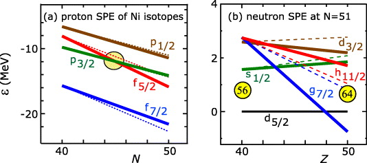
Figure 11. SPEs of (a) protons for Ni isotopes and (b) neutrons for N = 51 isotones calculated by VMU interaction. The dashed lines are obtained by the central force only, while the solid lines include both the central force and the tensor force. In (a), the yellow circle highlights the inversion between the 0f7/2 and 0f5/2 orbits. In (b), the numbers in the yellow circles indicate (sub-)magic gaps for Z = 40 and 50. Modified from figures 3(b) and (c) of [16].
Download figure:
Standard imageWe also note that the properties shown in figure 10 are consistent with observed results, and are important ingredients to recent studies on boundaries of the island of inversion. For example, the narrowing of N = 20 gap near Z = 8 moves the boundary from N = 20 to smaller values, or makes it obscure [10, 23].
Figure 11(a) shows proton SPEs for 68−78Ni starting from empirical values [24] at N = 40. The SPE of p1/2 is not known empirically, and is placed above p3/2 by the energy difference predicted by the GXPF1A interaction. The orbit f5/2 crosses p3/2 at N = 45 as marked on figure 11(a); consistent with a recent experiment [25]. The f7/2–f5/2 splitting is reduced by 2 MeV from N = 40 to 50. For both, the tensor force plays crucial roles. Apart from certain differences, the trend is seen in other shell model results, e.g., [26].
Figure 11(b) shows neutron SPEs relative to d5/2 on top of 90Zr–100Sn, starting from empirical values at Z = 40 obtained by averaging with spectroscopic factors (www.nndc.bnl.gov/ensdf/). The lowering of g7/2 is remarkable [27]. One finds a sub-magic gap at N = 56 for Z = 40 as shown in figure 11(b), while the gap is changed to N = 64 for Z = 50 as shown in the same figure. However, if there were no tensor-force effects, g7/2 and h11/2 do not repel, ending up with quite a different shell structure for 100Sn, making this nucleus much softer. The closer spacing of g7/2 and d5/2 in 101Sn seems to be seen experimentally [28].
There are more experimental data showing shell evolution phenomena, from light to medium-mass, e.g., of A ∼ 40 [29], and further to heavy, e.g., of A ∼ 150 [30], nuclei, as discussed in review papers, [31, 32].
We now discuss whether the simple tensor force in VMU can be explained microscopically or not. We take the AV8' interaction [33] and examine how the tensor force obtained by the spin–tensor decomposition changes in the following processes. We derive a low-momentum interaction Vlow k [34] and calculate vm, as shown in figures 12(a) and (b) for T = 0, 1, varying the cut-off parameter, Λ. For the usual value Λ = 2.1 fm−1, the result is very close to the bare AV8' tensor-force contribution. We then perform the third-order Q-box calculation with folded diagram corrections [18], in order to include medium effects like core polarization. The result still resembles vm of the bare tensor part. Thus we can confirm that the treatments of the short-range correlation and the medium effects do not change much vm of the tensor force. This near-independence has been formulated further by introducing the concept of Renormalization Persistency in [35]. Whereas the tensor force remains almost unchanged by the renormalization, the central force is changed substantially after the renormalization. For instance, the second-order perturbation by two tensor forces yield mainly a central force [35].

Figure 12. Tensor forces in AV8' interaction, in low-momentum interactions obtained from AV8', and in the third-order Qbox interaction for (a) T = 0 and (b) T = 1. Reprinted from [16]. Copyright (2010) by the American Physical Society.
Download figure:
Standard imageWe note that, for unusual values like Λ = 1 fm−1, the situation looks different, but is irrelevant to the present studies on actual structure of nuclei.
In contrast to the tensor force, the effective central force depends strongly on Λ. For Λ = 2.1 fm−1, vm of the central part of Vlow k are scattered around the values of figure 8(b). This result is promising, but more studies are needed.
6. Tensor force and single-particle strength distribution
We have seen that the tensor force changes spin–orbit splitting significantly, leading to tensor-force driven shell evolution. Despite the large and important change of spin–orbit splitting, its direct test including fragmentation of single-particle strength has not been presented. Such a test is rather difficult in most cases as one of the spin–orbit partners can be either deeply bound or unbound (or barely bound). We shall show, in this section, the first test of this kind for proton 0d5/2–0d3/2 spin–orbit splitting in 48Ca, comparing to spectroscopic factors measured in the (e,e'p) experiment [36].
This work has been performed in terms of shell-model calculations with a newly constructed Hamiltonian [37]. We first outline how this Hamiltonian is constructed. The sd and pf shells are taken as the valence shell with protons in sd and neutrons in pf. The interactions within each of these shells are based on existing interactions: USD [41] (GXPF1B [42]) for the sd (pf) shell, except for the monopole interactions VT=0,10d3/2,0d5/2 based on SDPF-M [10] due to a problem in USD as pointed out in [9]. The monopole- and quadrupole-pairing matrix elements  are replaced with those of KB3 [8]. This is mainly for a better description of nuclei of N ∼ 22. Although this replacement is not so relevant to the present study where N is larger in most cases, it has been made so that the applicability of the new Hamiltonian becomes wider. The cross-shell part, most essential for exotic nuclei discussed in this study but rather undetermined so far, is given basically by VMU of [16] with small refinements stated below. The tensor-force component is exactly from VMU, implying the π + ρ meson exchange force. It has been used in many cases [13, 16], and it has been accounted for microscopically under the new concept of Renormalization Persistency [35] where modern realistic effective interactions are analyzed in terms of the spin–tensor decomposition technique [38–40]. The central-force component of VMU interaction has been determined in [16] so as to reproduce monopole properties of shell-model interactions SDPF-M (sd-shell part) and GXPF1A [19, 20] by a simple Gaussian interaction. We introduce here slight fine tuning with density dependence similar to the one in [39], in order that its monopole part becomes closer to that of GXPF1B. We note that GXPF1B Hamiltonian [42] was created from GXPF1A Hamiltonian [20] by changing five T = 1 matrix elements and SPE involving 1p1/2, and that such differences give no notable change to the present work due to the minor relevance of 1p1/2. We include the two-body spin–orbit force of the M3Y interaction [43]. (For the present study, all these refinements produce minor changes, and do not change the overall conclusions. The refinements have been made so that the new Hamiltonian works well in a wide variety of nuclei other than those of this study.) Following USD and GXPF1B, all two-body matrix elements are scaled by A−0.3. The SPE of sd shell are taken from USD, and those of pf shell are determined by requesting their effective SPEs on top of 40Ca closed shell equal to the SPEs of GXPF1B.
The Hamiltonian, referred to as SDPF-MU hereafter2, is thus fixed prior to the shell-model calculations of this work. The diagonalization is performed by the mshell64 code [44].
We now come to the distribution of single-particle strength of proton sd-shell orbits. Spectroscopic factors obtained for 48Ca with the (e,e'p) reaction are displayed in the upper panels of figure 13 [36]. The 0d5/2 single-particle strength is highly fragmented due to its high excitation energy (3–8 MeV range). The spectroscopic factors obtained by the present calculation are shown in the lower left-hand panel of figure 13, where an overall quenching factor 0.7 is used following the standard recipe to incorporate various effects of components outside the valence shell [45]. The agreement is excellent both in the position of peaks and their magnitudes. However, this agreement is lost if the tensor force is removed from the cross-shell interaction, as shown in the right lower panel of figure 13. For instance, the largest 0d3/2 and 1s1/2 peaks are in the wrong order, and the strongest peaks of 0d5/2 move towards higher energy. The 0d3/2–0d5/2 gap of 48Ca turns out to be ∼5 MeV in the present calculation. This gap becomes ∼7 MeV for 48Ca, if the cross-shell tensor force is switched off, implying a reduction of ∼2 MeV due to the tensor force.

Figure 13. Spectroscopic factors of proton hole states measured by 48Ca(e,e'p) [36] (upper) and its theoretical calculation (lower left). The cross-shell tensor force is removed in lower right panel. The black, blue and red bars correspond to 1s1/2, 0d3/2 and 0d5/2 states, respectively. Reprinted from [37]. Copyright (2012) by the American Physical Society.
Download figure:
Standard imageFor 40Ca, although no experimental data by (e,e'p) reaction are available [46], Bastin et al suggested a reduction of proton 0d5/2–0d3/2 gap by 1.9 MeV from 40Ca to 48Ca based on reaction data [52]. Effective SPEs obtained from the SDPF-MU Hamiltonian are consistent with this and other experimental data [31, 32]. On the other hand, the gap remains almost unchanged between 40Ca and 48Ca, if the tensor force is removed from the cross-shell part of SDPF-MU Hamiltonian. We note that the spectroscopic factor distributions for 0d3/2 and 1s1/2 were calculated also by a Green's function method by Barbieri [45], but there has been no previous report on the 0d5/2 strength.
The proton shell structure thus evolves from 40Ca to 48Ca. Because only the tensor force can change the 0d3/2–0d5/2 gap by this order of magnitude (∼2 MeV), the agreement shown in figure 13 provides us with the first evidence from electron scattering experiments to the tensor-force-driven shell evolution induced by the mechanism of Otsuka et al [13]. This agreement implies also the validity of the present SDPF-MU Hamiltonian, especially the interaction between the proton sd and neutron pf shells.
7. Structure of exotic Si and S isotopes
We now move to the shape transitions in exotic Si (Z = 14) and S (Z = 16) isotopes with even N = 22–28 [37]. We shall show that tensor-driven shell evolution plays a critical role in the rapid shape transition as a function of neutron and/or proton number, including triaxial and γ-unstable shapes. In particular, we show for the first time3 how this shape transition at low energy can be related to the Jahn–Teller type effect [48, 49], where a geometric distortion is brought about by a particular coherent superposition of relevant single-particle states enhanced due to their (near) degeneracy.
We show calculated energy levels and B(E2) values for the Si and S isotopes that are in good agreement with experiments where they exist4 [50–55], and new predictions are made. Potential energy surfaces (PESs) for the Si and S isotopes for even N = 22–28 are shown. The PES changes rapidly as a function of neutron number, and are different for Si and S. The PES for 42Si shows a strong oblate shape (rather than spherical) due to the tensor-force-driven shell evolution. These PES results are interpreted in an intuitive picture involving shell gaps and the Jahn–Teller-type effect. At the end of this section we show that the calculated two-neutron separation energies are also in good agreement with experiment, and discuss the reasons for this.
The present shell-model Hamiltonian, called SDPF-MU, has been constructed from the VMU interaction, as described in detail in the previous section. The VMU interaction has been used also to construct the cross-shell part of a recent shell-model Hamiltonian for p–sd shell nuclei including neutron-rich exotic ones [56], similarly to the construction of the present SDPF-MU Hamiltonian. This new p–sd Hamiltonian works well in very light (B,C,N,O) nuclei. The VMU interaction is consistent, particularly for its monopole component, with successful shell-model interactions in sd (USD, SDPF-M) and pf (GXPF1A) shells [16], by construction. For the present study it is of interest to examine the validity of this general approach up to medium-mass (Si–S) nuclei, foreseeing further applications to heavier nuclei.
Before discussing quantitative results, we present an intuitive picture in figure 14 on the relation between the shell structure and the shape of Si nuclei. To begin with, we consider only two orbits 0d5/2 and 1s1/2 of protons for the sake of simplicity. In a conventional view, Z = 14 is a sub-magic number: no mixing between 1s1/2 and 0d5/2 due to large 1s1/2–0d5/2 gap and/or weak mixing force. Six protons occupy all states of 0d5/2 forming a closed subshell, as depicted in figure 14(a). This should end up with a spherical shape for a doubly magic nucleus, 42Si (N = 28), similarly to 34Si (N = 20).

Figure 14. Intuitive illustration of the structure of intrinsic state at Z = 14. Single-particle states of magnetic quantum numbers, denoted m, are shown. q implies intrinsic quadrupole moment (fm2) obtained with harmonic oscillator ℏω = 11.8 MeV. Reprinted from [37]. Copyright (2012) by the American Physical Society.
Download figure:
Standard imageFigure 14(b) indicates another situation where sizable mixing occurs between the 1s1/2 and 0d5/2 orbits in the case when the proton–neutron correlation is stronger than in figure 14(a) and competes with 1s1/2–0d5/2 spacing. The proton–neutron interaction, apart from its monopole part, can be modeled by a quadrupole–quadrupole interaction to a good extent. Effects of this interaction can be discussed in terms of intrinsic states due to a quadrupole deformation. Assuming an axially symmetric deformation, single-particle states of the same magnetic quantum numbers, denoted m, are mixed in the intrinsic states. Figure 14(b) shows that this occurs for m = ± 1/2 between 1s1/2 and 0d5/2, with amplitudes sin θ and cos θ, respectively. The phase of the mixing amplitude depends on the shape, prolate or oblate. In the case of Si isotopes, protons occupy the states of m = ± 5/2,±3/2, which yield in total a negative intrinsic quadrupole moment (oblate). The total intrinsic quadrupole moment gains a larger magnitude, if the 1s1/2–0d5/2 mixing gives a negative moment. The contribution from the proton–neutron multipole interaction to the energy of total intrinsic state is proportional approximately to the product of the proton intrinsic quadrupole moment and the neutron one. Because a similar situation can occur for neutrons in 1p3/2 and 0f7/2 with a negative intrinsic moment produced mainly by the m = ± 7/2 component of 0f7/2, a stronger binding is obtained for the total intrinsic state with an oblate shape. Although the proton 0d3/2 orbit is mixed to some extent in the actual shell-model calculation, the above mechanism still holds: the occupation of m = ± 5/2 remains with large negative quadrupole moment (oblate), and the mixing can occur among 0d5/2, 0d3/2 and 1s1/2 orbits in the relevant m = ± 1/2 and ±3/2 components in favor of the oblate shape.
One may wonder at the relation to the prolate deformation which dominates the shape of deformed nuclei. Figure 15 exhibits how the prolate shape is favored. Here, we assume two protons occupying 0d5/2 and 1s1/2 orbits. In this case, the magnitude of intrinsic quadrupole moment can be larger by mixing properly m = ± 1/2 states of 0d5/2 and 1s1/2 orbits rather than allocating them into m = ± 5/2 states. Thus, the present picture is consistent with the prolate dominant feature of nuclear shape.

Figure 15. Intuitive illustration of the appearance of prolate deformation. See the caption of figure 14.
Download figure:
Standard imageThe mechanism being discussed is of Jahn–Teller type, and it works if the mixing due to the proton–neutron correlation can compete with SPE spacings. The above intuitive pictures with figures 14(a) and (b) suggests rather robustly that the shape of 42Si can be spherical or oblate, but not prolate. The 0d5/2–1s1/2 spacing is 7.8 MeV for 42Si with the SDPF-MU Hamiltonian in the filling scheme. This is indeed comparable with the ground-state expectation value, −13.2 MeV, of multipole proton–neutron interaction, obtained by the shell-model calculation discussed below. Regarding the tensor force, when many neutrons occupy the 0f7/2 orbital, the proton 0d5/2 is raised due to the mechanism of Otsuka et al [13] discussed for the (e,e'p) data in the previous section. This effect is included in the result of SDPF-MU Hamiltonian, reducing 0d5/2–1s1/2 spacing by 1.1 MeV for 42Si. We shall see its importance now.
We here investigate quantitatively the structure of Si and S isotopes in the context of the shell-model calculations with the SDPF-MU Hamiltonian. Figure 16 exhibits properties of even-A Si and S isotopes. Effective charges are (ep,en) = (1.35e,0.35e) where an isoscalar shift fixed for lighter isotopes is taken. The overall agreement with experiment is excellent in figure 16. For instance, in the present result, 2+1 levels of Si isotopes keep coming down as N increases consistently with experiment. The nice agreement suggests that the intuitive picture with figure 14(b) works particularly well towards 42Si, resulting in a strongly deformed shape with low excitation energies consistent also with recent measurement in GANIL [52]. However, if the tensor force is omitted from the cross-shell interaction, the 2+1 level of 42Si goes up, suggesting the case in figure 14(a). Figure 16 exhibits results for S isotopes also in good overall agreement, including a bumpy behavior of the 4+1 level. Earlier shell-model calculations with empirical interactions [22, 57] give larger deviations and/or different trends from experiments. Different Hamiltonians are taken in [22] between Z ⩽ 14 and Z ⩾ 15 isotopes related to the monopole pairing strength in pf shell. The deviation from experiment becomes larger if this change is switched off. The present Hamiltonian is the same for all isotopes, and has been fixed prior to the shell-model calculations so as to make predictions. It is of much interest to see the missing experimental data in figure 16 as well as more precise B(E2) values.

Figure 16. (a), (b) 2+1,2 (blue lines and red circles) and 4+1 (green lines and red triangles) energy levels and (c), (d) B(E2;0+1 → 2+1) values of Si and S isotopes for N = 22–28. Symbols are experimental data (see footnote 4)) [50–55]. Solid (dashed) lines are calculations with (without) the cross-shell tensor force. Reprinted from [37]. Copyright (2012) by the American Physical Society.
Download figure:
Standard imageThe PES can be used to understand shapes contained in theoretical calculations. Figures 17 and 18 exhibit PES for Si and S isotopes, respectively, obtained by the constrained Hartree–Fock method [58] for the SDPF-MU Hamiltonian. The full Hamiltonian is taken in panels ((a)–(d)) of the two figures, whereas the cross-shell tensor force is removed in panels (e–h) of them. Let us start with PESs of Si isotopes (figure 17). Shape evolutions are seen very clearly in both sequences ((a)–(d)) and ((e)–(h)), starting with similar patterns in 36Si. The shape evolves as more neutrons occupy pf-shell, with distinct differences between the two sequences. In (b) and (c), the deformation becomes stronger from (a) with triaxial minima, whereas the shape becomes more like modestly prolate in (f) and (g). In (d), one finds a strongly oblate shape with a sharp minimum, but the minimum is at the spherical shape in (h). This strong oblate deformation produces low 2+ level and large B(E2) in figure 16 for the 'doubly-closed' 42Si. Thus, the shape of exotic Si isotopes changes significantly within the range of ΔN ∼ 6. This feature is partly due to growing collectivity with more neutrons in the pf shell, but is also a manifestation of Jahn–Teller-type effect driven by the tensor force. Without the tensor force, the SPE spacings are too large, and the correlation energies cannot produce this effect.
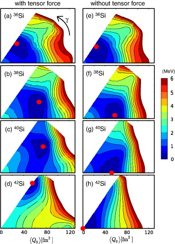
Figure 17. PES of Si isotopes from N = 22 to 28 calculated with (left) and without (right) the cross-shell tensor force. The energy minima are indicated by red circles. Reprinted from [37]. Copyright (2012) by the American Physical Society.
Download figure:
Standard image
Figure 18. PES of S isotopes from N = 22 to 28. See the caption of figure 17. Reprinted from [37]. Copyright (2012) by the American Physical Society.
Download figure:
Standard imageThe γ-unstable deformation is well developed in figure 17(c), and this can be confirmed by the low-lying 2+2 level of 40Si in figure 16. This level seems to agree with a recent γ-ray experiment [51] where either of γ-rays 638(8) and 845(6) keV appears to feed directly the 2+1 state. We stress that the 2+2 level is sensitive to the tensor force through γ-instability in Si isotopes. In fact, the ratio Ex(2+2)/Ex(2+1) is as low as 1.5 for 40Si, whereas it becomes 4.4 for 42Si. The former is a prominent signature of γ-instability, while the latter is consistent with a vibration from a profound PES minimum of axially-symmetric deformation. Thus, the change from 40Si to 42Si is an intriguing example of the rapid and unexpected structure evolution. If the tensor force is switched off in the cross-shell interaction, Ex(2+1) of 42Si is raised but B(E2) value is still larger than that of 40Si. This is partly due to the stretched minimum in figure 17(h) and partly due to relatively enhanced proton contribution in the E2 transition because of N = 28 closure.
The situation is quite different with PES of S isotopes (figure 18). With two more protons added to Si isotopes, the occupancy of the 0d5/2 orbit is closer to that of a closed shell. The mixing between 1s1/2 and 0d3/2 then plays a decisive role, leading to a structure favoring prolate deformation. As for neutrons, m = ± 7/2 components of 0f7/2 carry large negative intrinsic quadrupole moment and are crucial for oblate shape, while the others have positive or small negative values. In S isotopes, as protons favor prolate shapes, neutron sector becomes prolate for N < 28, by keeping the m = ± 7/2 states (almost) unoccupied and having proper occupations and mixings of other states. At N = 28, the m = ± 7/2 states are occupied more. However, the neutron 0f7/2–1p3/2 spacing decreases from Ca isotopes to Si and S ones due to the vacancy of proton 0d3/2, and the excitation from the m = ± 7/2 states to other orbits does not cost much energy as compared to gains from proton–neutron correlation. This gives rise not to an oblate minimum but to triaxial softness. Thus, the shape is determined, in the present cases, primarily by the proton sector. We would like to emphasize the crucial role of protons in determining shapes of Si and S isotopes. Future measurements of quadrupole moments of these nuclei will be of high interest.
We comment also that the quasi SU(3) scheme [59, 60] favors an oblate shape at N = 28, with a prolate state slightly higher than this. The quasi SU(3) is constructed for the configurations comprised of almost degenerate j and j − 2 orbits only, e.g., 0f7/2 and 1p3/2.
The difference of the shapes between Si and S isotopes may suppress transfer reactions, for instance, two-proton removal from 44S [61].
We now discuss two-neutron separation energies (S2n) shown in figure 19. The agreement between experiment and the full calculation is quite good within ∼0.5 MeV, except for N = 22 Si value with discrepancy of 1.2 MeV due to the mixing of intruder configurations in 34Si, an issue outside this work. If the tensor force is switched off, deviations of 1–3 MeV occur for Si and S isotopes in the direction of larger S2n values. This means that the tensor-force effect is repulsive and becomes larger from Ca to Si isotopes as a whole, consistently with the tensor-force-driven shell evolution. This evolution induces stronger deformation in some cases, e.g. 42Si, where additional binding energy is gained and can cancel partly this repulsive effect. Thus, the tensor force plays quite important roles also on binding energies, while it seems to have been somewhat overlooked.

Figure 19. Two-neutron separation energies of Si and S isotopes from N = 22 to 28. Solid (dashed) lines are calculations with (without) the cross-shell tensor force. Points are experimental data [62, 63]. Reprinted from [37]. Copyright (2012) by the American Physical Society.
Download figure:
Standard imageWhile Si and S isotopes have been discussed with density-functional methods including appearance of oblate shapes [64–67], there are problems to be solved. No systematic calculations have been reported for levels and B(E2) of Si isotopes. The 2+1 level calculated in [67] reproduces experiment for 44S, but deviates by a factor of two for 42Si. Figures 16(a) and (b) shows that the 2+1 level of 42Si is sensitive to the tensor force, whereas that of 44S is not. The difference between 42Si and 44S in [67] might be relevant to this. The systematics of 2+1 level in S isotopes shows opposite trend in [66]. It will be also of interest to see single-particle properties given by these works. For instance, the proton 0d5/2–0d3/2 gap remains almost unchanged from 40Ca to 48Ca in these calculations, but this contradicts the trend seen in (e,e'p) data [36].
8. Three-body force
We now turn to another major subject, three-body force, based on [3, 68]. Figure 1 shows that the neutron drip line evolves regularly with increasing proton number, with an odd–even bound–unbound pattern due to neutron halos and pairing effects. The only known anomalous behavior is present in the oxygen isotopes, where the drip line is strikingly close to the stability line [69]. Already in the fluorine isotopes, with one more proton, the drip line is back to the regular trend [70]. In this paper, we discuss this puzzle and show that three-body forces are necessary to explain why the doubly-magic 24O nucleus [71, 72] is the heaviest oxygen isotope.
Three-nucleon (3N) forces were introduced in the pioneering work of Fujita and Miyazawa (FM) [73] and arise because nucleons are composite particles, with resonances that can be excited by other nucleons. The FM 3N mechanism is due to one nucleon virtually exciting a second nucleon to the Δ(1232 MeV) resonance, which is de-excited by scattering off a third nucleon, see figure 20(e).

Figure 20. Processes involved in the discussion of 3N forces and their contributions to the monopole components of the effective interactions between two valence neutrons. The solid lines denote nucleons, the dashed lines denote pions, and the thick lines denote Δ excitations. Nucleon–hole lines are indicated by downward arrows. The leading chiral 3N forces include the long-range two-pion-exchange parts, diagram (f), which take into account the excitation to a Δ and other resonances, plus shorter-range one-pion exchange, diagram (g), and 3N contact interactions, diagram (h). Reprinted from [3]. Copyright (2010) by the American Physical Society.
Download figure:
Standard imageThree-nucleon interactions arise naturally in chiral effective field theory (EFT) [74], which provides a systematic basis for nuclear forces, where nucleons interact via pion exchanges and shorter-range contact interactions. The resulting nuclear forces are organized in a systematic expansion from leading to successively higher orders, and include the Δ excitation as the dominant part of the leading 3N forces [74]. The quantitative role of 3N interactions has been highlighted in recent ab-initio calculations of light nuclei with A = N + Z ⩽ 12 [75, 76].
We first discuss why the oxygen anomaly is not reproduced in shell-model calculations derived from microscopic NN forces. This can be understood starting from the stable 16O and adding neutrons into single-particle orbitals above the 16O core. We will show that correlations do not change this intuitive picture. Starting from 16O, neutrons first fill the 0d5/2 orbitals, with a closed subshell configuration at 22O (N = 14), then the 1s1/2 orbitals at 24O (N = 16), and finally the 0d3/2 orbitals at 28O (N = 20). For simplicity, we will drop the nodal quantum number in the following.
In figure 21, we show the SPE of the neutron d5/2, s1/2 and d3/2 orbitals at subshell closures N = 8, 14, 16 and 20. The evolution of the SPE is due to interactions as neutrons are added. For the SPE based on NN forces in figure 21(a), the d3/2 orbital decreases rapidly as neutrons occupy the d5/2 orbital, and remains well-bound from N = 14 on. This leads to bound oxygen isotopes out to N = 20 and puts the neutron drip line incorrectly at 28O. This result appears to depend only weakly on the renormalization method or the NN interaction used. We demonstrate this by showing SPE calculated in the G-matrix formalism [77], which sums particle–particle ladders, and SPE based on low-momentum interactions Vlow k [34] obtained from chiral NN interactions at next-to-next-to-next-to-leading order (N3LO) [78] using the renormalization group. Both results include core polarization effects perturbatively (to second order) and start from empirical SPE [10] in 17O. We emphasize that the empirical SPE include also 3N contributions (from the core) that can be calculated in ab-initio approaches in the future.

Figure 21. SPE of the neutron d5/2, s1/2 and d3/2 orbitals measured from the energy of 16O as a function of neutron number N. Panel (a) presents the SPE calculated from a G-matrix and from low-momentum interactions Vlow k. Panel (b) shows the SPE obtained from the phenomenological forces SDPF-M [10] and USD-B [79]. The contributions from 3N forces due to Δ excitations and all chiral EFT 3N interactions at N2LO [83]6 are included in panels (c) and (d). The changes due to 3N forces based on Δ excitations are highlighted by the shaded areas. Reprinted from [3]. Copyright (2010) by the American Physical Society.
Download figure:
Standard imageIn order to understand the oxygen anomaly, we show in figure 21(b) the SPE obtained from the phenomenological forces SDPF-M [10] and USD-B [79] that have been fit to reproduce experimental binding energies and spectra. This shows a striking difference compared to figure 21(a): as neutrons occupy the d5/2 orbital, with N evolving from 8 to 14, the d3/2 orbital remains almost at the same energy and is not well-bound out to N = 20. The dominant differences between the microscopic results of figure 21(a) and those obtained from phenomenological forces can be traced to the monopole components of two-body interaction (see equation (1)), which is nothing but the average interaction between two orbits.
The comparison of figures 21(a) and (b) suggests that the monopole interaction between the d3/2 and d5/2 orbitals obtained from NN theories is too attractive, and that the oxygen anomaly can be solved by additional repulsive contributions to the two-neutron monopole components, which approximately cancel the average NN attraction on the d3/2 orbital. With extensive studies based on NN forces, it is unlikely that such a distinct property would have been missed, and it has been argued that 3N forces may be important for the monopole components [80].
In fact, figures 8(c) and (d) indicate that monopole components are modified to be more repulsive from G-matrix to GXPF1A in pf shell, except for only one case with j = j' = f5/2. Since GXPF1A reproduces the experimental data well, this general trend can be a clear hint as to what is missing in the microscopic NN interaction (G-matrix in this case) systematically. The situation is the same in the sd shell as shown in figures 8(g) and (h). We thus conclude that there should be certain mechanism which makes T = 1 effective NN interaction more repulsive in general.
Next, we show that 3N forces between two valence neutrons and one nucleon in the 16O core give rise to repulsive monopole interactions between the valence neutrons. While the contributions of the FM 3N force to other quantities can be different, the shell-model configurations composed of valence neutrons probe the long-range parts of 3N forces. The repulsive nature of this 3N mechanism can be understood based on the Pauli exclusion principle. Figure 20(a) depicts the leading contribution to NN forces due to the excitation of a Δ, induced by the exchange of pions with another nucleon. Because this is a second-order perturbation, its contribution to the energy and to the two-neutron monopole components has to be attractive. This is part of the attractive d3/2–d5/2 monopole component obtained from NN forces.
In nuclei, the process of figure 20(a) leads to a change of the SPE of the j,m orbital due to the excitation of a core nucleon to a Δ. This is illustrated in figure 20(b) by the Δ–nucleon–hole loop and the initial neutron is virtually excited to another j',m' orbital. As discussed, this lowers the energy of the j,m orbital and thus increases its binding. However, in nuclei this process is forbidden by the Pauli exclusion principle, if another neutron occupies the same orbital j',m', as shown in figure 20(c). The corresponding contribution must then be subtracted from the SPE change due to figure 20(b). This is taken into account by the inclusion of the exchange diagram, figure 20(d), where the neutrons in the intermediate state have been exchanged and this leads to the exchange of the final (or initial) orbital labels j,m and j',m'.5 Because this process reflects a cancelation of the lowering of the SPE, the contribution from figure 20(d) has to be repulsive for two neutrons. Finally, we can rewrite figure 20(d) as the FM 3N force of figure 20(e), where the middle nucleon is summed over all nucleons in the core.
The changes in the SPE evolution due to 3N forces based on Δ excitations are shown in figure 21(c) for the G-matrix formalism, where a standard pion–nucleon–Δ coupling [81] was used and all 3N diagrams obtained from antisymmetrization are included. We observe that the repulsive FM 3N contributions become significant with increasing N and the resulting SPE structure is similar to that of phenomenological forces, where the d3/2 orbital remains high. Next, we consider the SPE calculated from chiral low-momentum interactions Vlow k and include the changes due to the leading (N2LO) 3N forces in chiral EFT [82], see figures 20(f)–(h), as well as due to Δ excitations7. The leading chiral 3N forces include the long-range two-pion-exchange part, figure 20(f), which takes into account the excitation to a Δ and other resonances, plus shorter-range 3N interactions, figures 20(g) and (h), that have been constrained in few-nucleon systems [83] (see footnote 5). The resulting SPE in figure 21(d) demonstrate that the long-range contributions due to Δ excitations dominate the changes in the SPE evolution and the effects of shorter-range 3N interactions are smaller. In addition, 3N forces play a key role for magic numbers, for the N = 14 gap between the d5/2 and s1/2 orbitals [84], and they enlarge the N = 16 gap between the s1/2 and d3/2 orbitals [72].
The contributions from figures 20(f)–(h) (plus all exchange terms) to the monopole components take into account the normal-ordered two-body parts of 3N forces, where one of the nucleons is summed over all nucleons in the core. This is also motivated by recent coupled-cluster calculations [85], where residual 3N forces between three valence states were found to be small. The inclusion of 3N multipole contributions changes the oxygen ground-state energies by less than 300 keV. In addition, the effects of 3N forces among three valence neutrons should be weak due to the Pauli principle.
We note that figures 20(a) and (e) are relevant to neutron matter and neutron star through the competition between the attraction from figure 20(a) and the repulsion from figure 20(e) [86]. This can be compared to the attraction in figure 20(b) and the repulsion in figures 20(c) and (d). Namely, neutron stars and exotic nuclei are subject to the same three-body force and similar mechanisms, whereas the density is high in the former but low in the latter.
Finally, we take into account many-body correlations by diagonalization in the valence space, including the 3N contributions to the monopole components. The resulting ground-state energies of the oxygen isotopes are presented in figure 22. Figure 22(a) (based on phenomenological forces fit to experiment) demonstrates that many-body correlations do not change our picture developed from the SPE: the energy decreases to N = 16, but the d3/2 neutrons added out to N = 20 remain unbound. Figures 22(b) and (c) give the energies derived from NN forces, using a G-matrix or low-momentum interactions Vlow k, and including 3N forces. For all results based on NN forces, the energy decreases to N = 20 and the neutron drip line is incorrectly located at 28O. The changes due to 3N forces based on Δ excitations are highlighted in figures 22(b) and (c). This leads to a better agreement with the experimental energies and to a kink at N = 16, which is further strengthened by shorter-range 3N interactions, and for low-momentum interactions corresponds to the location of the neutron drip line at 24O.
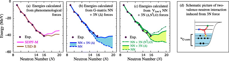
Figure 22. Ground-state energies of neutron-rich oxygen isotopes measured from the energy of 16O. The experimental energies of the bound oxygen isotopes 16−24O are included for comparison. Panel (a) shows the energies obtained from the phenomenological forces SDPF-M [10] and USD-B [79]. Panel (b) gives the energies obtained from a G-matrix and including FM 3N forces due to Δ excitations. Panel (c) presents the energies calculated from low-momentum interactions Vlow k and including all chiral EFT 3N interactions at N2LO as well as only due to Δ excitations [83] (see footnote 5). The changes due to 3N forces based on Δ excitations are highlighted by the shaded areas. (d) Schematic illustration of a two-valence-neutron interaction generated by 3N forces with a nucleon in the 16O core. Reprinted from [3]. Copyright (2010) by the American Physical Society.
Download figure:
Standard imageFluorine isotopes have one more proton than oxygen. Figure 10 shows that NN forces, primarily the tensor part, with this proton provide more binding to the valence neutrons [13, 87]. This valence proton–neutron effect is absent in the oxygen isotopes, making the repulsive 3N mechanism visible.
We have confirmed similar mechanism in exotic Ca isotopes, improving binding energies and affecting shell structure [88]. Important directions are to include the presented 3N contributions in coupled-cluster calculations and in density-functional calculations of all nuclei, to systematically explore the effect on the full range of the neutron drip line. In fact, recent coupled-cluster calculations in [89] show results consistent with those presented here and in [88].
9. Shell evolution in the continuum
The shell evolution continues from bound to continuum states. For instance, the location of d3/2 state remains in the continuum in oxygen isotopes, and appears as resonance (-like) state. The continuum effect pushes down its energy from the value obtained in the bound state approximation. The final combined result agrees quite well with experiment. Details of such studies in terms of Continuum Coupled Shell Model (CCSM) will be reported elsewhere [90].
10. Shell evolution in heavy nuclei
The shell evolution occurs generally, and affects the structure of heavy nuclei including collective states. We have carried out Monte Carlo shell-model calculations [91–93] on Xe and Ba nuclei, and confirmed that the shell evolution mechanism can be seen in the level structure of collective states [94].
11. Summary
In summary, I have presented novel and general properties of the tensor, central and three-body forces in exotic nuclei. There is paradigm shift with respect to the shell structure and magic number due to these nuclear forces, after another paradigm shift with respect to the density distribution or neutron halo [2]. This implies new landscape of the structure of atomic nuclei in entering frontiers of exotic nuclei. It also suggests that some properties of nuclear and/or hadronic forces can be seen in exotic nuclei rather clearly with more visible effects of hadrons such as pions and Δ particles. More interesting and intriguing features of the nuclear structure will be explored by developing physics of exotic nuclei by means of RI-beams.
Acknowledgments
The author thanks many colleagues for valuable discussions and collaborations, particularly, Drs. T Suzuki, M Honma, Y Utsuno, T Mizusaki, N Shimizu, K Tsukiyama, N Tsunoda, N Akaishi, B A Brown, M Hjorth-Jensen, A Schwenk, J D Holt, H Grawe, J P Schiffer and many others. This work was in part supported by MEXT Grant-in-Aid for Scientific Research (A) 20244022, and by Mitsubishi Foundation. This presentation has been supported by Global COE Program 'the Physical Sciences Frontier', MEXT, Japan.
Footnotes
- 1
For j = j' for identical nucleons, slightly different forms are used.
- 2
SDPF-MU interaction is available upon request to the author.
- 3
Limited and brief report of this work is presented in [47].
- 4
Evaluated Nuclear Structure Data File (ENSDF) www.nndc.bnl.gov/ensdf/
- 6
We use the 3N couplings fit to the 3H binding energy and the 4He radius for the smooth-cutoff Vlow k with Λ = Λ3N = 2.0 fm−1. The one-Δ excitation 3N force corresponds to particular values for the two-pion-exchange part [74].
- 5
In the case of j = j', the average over m and m' is restricted to states allowed by antisymmetry.
- 7
The one-Δ contribution also corresponds to the leading (NLO) 3N force in an EFT with explicit Δ fields [74].