

Abstract
The transport coefficients, namely thermal conductivity, viscosity and electrical conductivity, of CO2–CH4 mixture in and out of LTE are calculated in this paper. The calculation was based on local chemical equilibrium (LCE) and local phase equilibrium assumption. The 2-temperature composition results obtained with consideration of condensed phase in the previous paper (Part I) of this series were used in this calculation. The transport coefficients were calculated by classical Chapman–Enskog method simplified by Devoto. The results are presented for different temperatures (300–30 000 K), pressures (0.1–10 atm), non-equilibrium degrees (1–5), and CH4 molar proportions (0–100%). The influence of condensed graphite, non-LTE effect, mixture ratio and pressure on the composition and thermodynamic properties has been discussed. The results will serve as reliable reference data for computational simulation of CO2–CH4 plasmas.
Export citation and abstract BibTeX RIS
1. Introduction
In many electrical devices, the inefficiency of electron–heavy-species collisions and the large temperature gradient may limit the redistribution of energy from the electrons and may cause the electron temperature differing from that of the heavy species, namely non local thermodynamic equilibrium (non-LTE) effect. In order to consider this effect in arc plasma simulation, the 2-temperature transport coefficients are necessary.
Two theories are frequently adopted to obtain the 2-T transport coefficients: (1) Devoto [1, 2] developed a simplified theory that neglects the coupling between heavy species and electron; (2) Rat et al [3] developed a theory in which the coupling between heavy species and electron is considered. A recent study [4] showed that the consideration of coupling between heavy species and electron does not lead to significant changes in the non-equilibrium plasma transport coefficients, except for certain ordinary diffusion coefficients. Many papers have focused on the calculation of 2-T transport coefficients.
Besides the non-LTE effect, the multiphase effect can also significantly influence the plasma composition, as shown in the first paper of this series [5] and the paper of André et al [6], and further influence the transport coefficients. However, to our knowledge, all the published 2-temperature transport coefficients are calculated for pure gaseous system. In the section 2 of this paper, a new calculation method for transport coefficients of 2-T multiphase system under local chemical equilibrium (LCE) and local phase equilibrium assumption is presented. The composition for multiphase system is obtained by the method presented by [5] using mass action law and the second law of thermodynamics. However, because there has been no proper theory to date to describe the interaction of condensed species, only the contribution of gaseous species to transport coefficient is considered. Considering the calculation efficiency, in this paper the simplified approach proposed by Devoto is used. A particular attention was paid to the elastic collisions using a phenomenological description of interaction potentials.
The CO2 and CO2 based mixture are considered to be substitute gases for SF6, which shows high global warming potential (GWP). Much research has been conducted on CO2 and CO2 based mixture as a substitute gas for SF6 [7–11]. In section 3, the transport coefficients of CO2–CH4 mixture, which shows environmental friendliness and good electrical properties [12], are calculated. The composition data are taken from the first paper of this series. The results are presented for different temperatures (300–30 000 K), pressures (0.1–10 atm), non-equilibrium degrees (1–5), and CH4 molar proportions (0–100%). Results for LTE composition and thermodynamic transport properties are in good agreement with previously published data. The influence of condensed graphite, non-LTE effect, mixture ratio and pressure on the thermo-physical properties has been discussed. The results will serve as reliable reference data for computational simulation of the behavior of CO2–CH4 plasmas. Some of the calculation results are tabulated in appendix.
2. Calculation method
2.1. Transport coefficients
The transport coefficients, namely viscosity, thermal conductivity and electrical conductivity, were calculated using the classical Chapman–Enskog method [13, 14], which assumes that the particle distribution function is a first-order perturbation to the Maxwellian distribution. The perturbations are expressed in series of Sonine polynomials, finally leading to a system of linear equations that can be suitably solved to obtain different transport properties. In a non-LTE system, a parameter of thermal non-equilibrium can be defined as θ = Te/Th, where Te and Th are respectively the electron and heavy-species temperatures.
Different approaches have been proposed to deal with the 2-T transport properties in partially-ionized plasmas. Among these, two main methods are frequently used: Devoto [1, 2, 15–17] developed a simplified theory neglecting the collisional coupling between heavy species and electrons, whereas Rat et al [3] developed a method that retains the coupling. It should be noted that coupling between electrons and heavy species does not lead to significant changes in the predicted non-equilibrium plasma transport properties, except for certain ordinary diffusion coefficients [4]. In the current work, the simplified approach of Devoto has been used, with a third-order approximation for diffusion coefficients, thermal conductivity and electrical conductivity. The same method has been used for calculating the viscosity, for which the second-order approximation has been adopted.
Among these transport coefficients, special attention had to be paid to the thermal conductivity. Thermal conductivity depends on the translation of electrons (λtre), the translation of heavy species (λtrh), internal energy changes (λin) and chemical reactions (λreac). The total thermal conductivities for electrons and heavy species can be evaluated by

The translational thermal conductivities (λtr e and λtr h) were calculated according to the method of Devoto [1, 15] in the third approximation of Sonine polynomial terms:
where the qmp and  are computed from associated collision integrals [1, 15].
The presence of internal degrees of freedom can affect the heat flux vector and therefore gives rise to an internal thermal conductivity, which is derived using the Hirschfelder–Eucken approximation [14]:
where Cpi is the specific heat at constant pressure of the species i,  and
and  are respectively the self-diffusion coefficient and the binary diffusion coefficient between species i and species j, and R, xi and w respectively denote the ideal gas constant, the mole fraction of species i, and the total number of species.
Chemical reactions lead to an additional heat flux, which introduces an additional reactive thermal conductivity component. A general expression of total reactive thermal conductivity with good applicability to monatomic, diatomic and polyatomic gases in terms of a two temperature model is utilized [18]:
where v and Δhr are, respectively, the number of chemical reactions and reaction enthalpy change of reaction r. The Hr and H are matrix derived by generalized Saha equations, Guldberg–Waage equations, the species diffusion velocities and Van't Hoff's equation modified for the two-temperature plasmas [18, 19].
The viscosity and electrical conductivity are obtained following the derivation presented by Devoto [15], which are given by
The coefficients  and qmp are given in the previously published paper [15].
2.2. Collision integrals
Expressions for transport properties contain determinants that depend on collision integrals, which are averages over a Maxwellian distribution of the collision cross–sections for the binary interactions between species [13, 14]. Collision integrals for the interaction between species i and j are defined as
where γ is the reduced initial speed of the colliding molecules i and j. gij and μij are the initial relative speed and reduced mass (given by  =
=  +
+  ) of the colliding species i and j. For non-equilibrium plasmas, collision integrals have to be calculated using a reduced temperature
  , given in equation (9).
  is the transport cross section, which can be derived from interaction potentials.
Each encounter between particles can be classified in to one of four types: (A) neutral–neutral encounters; (B) neutral–ion encounters; (C) electron–neutral encounters; (D) encounters between charged particles. For different types of encounter, the different interaction potentials have been adopted.
2.2.1. Neutral–neutral interactions.
Many types of intermolecular potential have been used to determine the collision integrals for interactions between neutral species [4, 8, 20–23]. Recently, a phenomenological model potential developed by Capitelli and co-workers has been widely studied [24, 25]. This phenomenological potential allows direct evaluation of internally-consistent complete sets of collision integrals for different atmospheres and can provide more accurate estimation of the interaction potential by recent comparative study performed for some benchmark system. Therefore, we adopt the phenomenological potential to calculate neutral–neutral collision integrals.
This model potential can be defined in terms of fundamental physical properties of involved interacting partners (polarizability  ). Most values used in this paper for heavy species are taken from the NIST Computational Chemistry Comparison and Benchmark Database [26]. All the polarizability data used in this calculation are given in table 1.
Table 1. Polarizability of neutral species.
| Species | α (Å) | Species | α (Å) | Species | α (Å) |
|---|---|---|---|---|---|
| C3 | 5.002 | C2H2 | 3.485 | H2O | 1.453 |
| C2 | 7.256 | C2H | 3.794 | HO2 | 1.983 |
| C | 1.286 | CH4 | 2.523 | OH | 1.113 |
| H2 | 0.822 | CH3 | 2.436 | COOH | 3.972 |
| H | 0.693 | CH2 | 2.263 | H2CO | 3.095 |
| O3 | 2.765 | CH | 2.518 | HCOOH | 3.369 |
| O2 | 1.559 | CO2 | 2.545 | CH3OH | 3.206 |
| O | 0.678 | C2O | 4.031 | HCO | 2.596 |
| C2H6 | 4.307 | CO | 1.955 | C2H4O | 4.916 |
| C2H4 | 4.152 | H2O2 | 2.279 | C2H5OH | 5.043 |
2.2.2. Ion–neutral interactions.
For neutral–ion interactions, two kinds of processes should be taken into account, which are purely elastic collisions and the resonant charge–exchange inelastic process. For l odd (l = 1 or 3), we followed the work of Murphy [27] and estimate the total collision integrals from the elastic and inelastic contributions with the empirical mixing rule:

where  is the inelastic collision integral and
  is the elastic interactions. The elastic collision integrals between neutral species and first order ions are obtained by adopting the phenomenological potential [24, 25]. The ions polarizability is taken from the NIST Computational Chemistry Comparison and Benchmark Database [26] and presented in table 2. For the elastic collision integrals between neutral species and high order ions, the polarization potential is adopted.
Table 2. Polarizability of first order ions.
| Species | α (Å) | Species | α (Å) |
|---|---|---|---|
| C+ | 0.899 | O+ | 0.388 |
 |
0.447 | CO+ | 1.337 |
 |
2.836 | OH+ | 0.599 |
 |
3.223 | OH− | 3.944 |
 |
0.97 | HCO+ | 1.44 |
| O− | 2.164 |
As given in equation (10), the inelastic interaction is taken into account in collision integral calculation. The charge-transfer cross section is approximated in the form

where E is the collision energy. The constants A and B can be obtained from experimental data or theoretical calculations. The data of interactions between C–C+, H–H+ and O–O+ are taken from the work by Copeland and Crothers [28], which agrees well with the data presented by Laricchiuta [29] and Eletskii [30]. For the charge exchange interactions between neutral atom and its negative ion, no accurate experimental data or theoretical calculations were found in the literature. The constants A and B have been determined using an empirical formula [31].
Laricchiuta [29] showed that charge exchange cross section of neutral-multiply charged ion interaction could be relevant especially for divalent ion and trivalent ion. However, this effect is not taken into account in the present paper, due to the small possibility of simultaneous presence of neutral species and multiply charged ions. Besides, the charge exchange cross sections for collisions between unlike species are small compared to the elastic collision integrals and are neglected in this paper.
The internal excited state may affect the many kinds of collision integrals and then may affect the transport coefficients [32, 33]. However, according to [32, 33], the influence of internal excited state on transport coefficients is relatively small when pressure is lower than 10 atm. Therefore, we believe that the results presented in this paper, which are lower than 10 atm, are not perfectly accurate but still reliable. To our knowledge, little papers of thermo-physical properties calculation considered the effect of internal excited state on collision integrals and transport coefficients. The importance of this effect is underestimated and needs more attention. In our further research work, we will focus on the effect of internal excited state on the collision integrals and transport properties under different condition.
2.2.3. Electron–neutral interactions.
For the e–C, e–H and e–O interactions, we use the techniques recommended by Laricchiuta et al [29] to determine transport cross sections. The electron–neutral cross sections, including the interaction between electron and C2, C2H2, C2H4, C2H6, C3, CH, CH2, CH3, CH4, CO, CO2, H2, H2O and O3 are mainly taken from Plasma Data Exchange Project [34]. The cross section of e–O2 is taken from numerical results proposed by Capitelli [23]. Other electron–neutral species collision integrals are calculated using the polarization potential.
2.2.4. Charged species interactions.
As presented in [23], the collision integrals for this interaction are known either in tabular form by Hahn [35] or approximated with closed forms presented by Liboff [36]. Devoto's work [37] shows that different definition of Debye length can significantly affect the charged–charged interactions and further affect the transport coefficients. In the present work, we used the method presented by Liboff with the Debyle length without consideration of ions, following the recommendation of Murphy [38] who found that without consideration of ions in Debye length calculation, the calculated argon electrical conductivity agrees better with the measured value. The Debye length without consideration of ions is given by
where ε0 is the vacuum electric permittivity and e is the elementary charge.
3. Transport coefficients of CO2–CH4 mixture
3.1. Transport coefficients under LTE assumption
Considering the close interrelationship between composition and transport coefficients, a brief analysis of reactions and composition in CO2–CH4 mixture is necessary before researching the transport coefficients. Figure 1(a) shows the composition of 50%CO2–50%CH4 mixture composition under LTE at atmospheric pressure. The reaction CO2 + CH4 ↔ 2H2O + 2C(c) makes H2O and graphite being the dominant species at low temperature (lower than 1000 K). After the sublimation of graphite at around 1200 K, the reaction CO2 + CH4 ↔ 2CO + 2H2 leads the domination of CO and H2. At 3200 K and 6800 K, H2 and CO dissociate respectively. The first order ionization of C, H and O occur at 12 500 K, 14 700 K and 15 700 K respectively. The second order ionization of C occurs at 27 000 K.
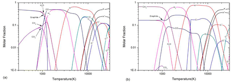
Figure 1. Temperature dependence of (a) 50%CO2–50%CH4 and (b) 10%CO2–90%CH4 mixture composition under LTE at atmospheric pressure
Download figure:
Standard image High-resolution imageThe mixture ratio can significantly affect chemical reaction and composition, especially the condensed species. Figure 1(b) shows the composition of 10%CO2–90%CH4 mixture at atmospheric pressure under LTE. Similar to 50%CO2–50%CH4 mixture, at low temperature (lower than 1000 K), the reaction CO2 + CH4 ↔ 2H2O + 2C(c) produces graphite and H2O. However, due to the low ratio of CO2, CH4 is the dominant species in this temperature range. As temperature increases, the CH4 dissociates into graphite and H2 and therefore there is an increase of graphite molar fraction at 1300 K. At around 4100 K, the graphite fully sublimates and phase transition process completes.
Figure 2 shows the electrical conductivity of CO2–CH4 mixtures with different ratio under LTE at atmospheric pressure. The mixture ratio can affect electrical conductivity especially at temperature lower than 15 000 K and higher than 23 000 K. Due to the low temperature of C ionization (12 500 K), the ionization process is dominated by C+ in low temperature. Therefore the increase of CO2 ratio causes increase of electron number density and further increases the electrical conductivity. When temperature is higher than 23 000 K, the high order ionization of C and O enhances the coulomb interaction and therefore lowers the electron mobility degree. Due to this phenomenon, the presence of CO2 in CO2–CH4 mixtures decreases the electrical conductivity. Our results show good agreement with that of Aubreton [39] and Yang [10].
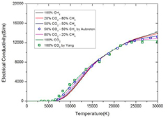
Figure 2. Temperature dependence of the electrical conductivity of CO2–CH4 plasmas with different molar proportions under LTE at atmospheric pressure. The results of Aubreton et al [39] and Yang et al [10] are shown with symbols for comparison.
Download figure:
Standard image High-resolution imageThe total thermal conductivity consists of four different parts namely heavy species translation thermal conductivity, electron translation thermal conductivity, internal thermal conductivity and reactive thermal conductivity. Figure 3 shows the components of total thermal conductivity of 50%CO2–50%CH4 plasmas at atmospheric pressure under LTE. The sharp peaks in total thermal conductivity are mainly caused by chemical reactions. The first peak at 1200 K is due to the phase transition and reaction CO2 + CH4 ↔ 2CO + 2H2. The other peaks at 3200 K, 6800 K and 15 000 K are due to H2 dissociation, CO dissociation, first order ionization respectively. The total thermal conductivity is dominated mainly by reactive and heavy species translational thermal conductivity at temperature under 10 000 K. In temperature range from 10 000 to 20 000 K, the total thermal conductivity is affected by both electron translational and reactive thermal conductivity. When the temperature is above 20 000 K, the total thermal conductivity is completely dominated by the electron translational component.
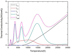
Figure 3. Components of total thermal conductivity of 50%CO2–50%CH4 plasmas at atmospheric pressure under LTE.
Download figure:
Standard image High-resolution imageThe mixture ratio can significantly affect the thermal conductivity, as shown in figure 4. The first peak at around 1000 K, which cannot be found in pure CO2 plasma, is due to the CH4 dissociation and reaction CO2 + CH4 ↔ 2CO + 2H2. The peaks at around 4000 K in different mixtures are due to the different chemical process. For the pure CO2, this peak is caused by CO2 dissociation. For CO2–CH4 mixture whose CO2 proportion is higher than 50%, this peak is due to the combination of CO2 and H2 dissociation. For 50% CO2–50%CH4 mixture, in which nearly all the CO2 is consumed by reaction CO2 + CH4 ↔ 2CO + 2H2 and there is no CO2 at 4000 K, this peak is the consequence of H2 dissociation only. For the CO2–CH4 mixture whose CH4 proportion is higher than 50%, the dramatic sharp peak at 4000 K is due to the H2 dissociation and graphite sublimation. The third peak which cannot be seen in pure CH4 is due to the CO dissociation. The highest peak value can be found in 50% CO2–50%CH4 mixture in which the molar fraction of CO is highest because of the reaction CO2 + CH4 ↔ 2CO + 2H2. Our results for pure CO2 consist well with Yang et al [10]. However, our results are significantly lower than Aubreton's results [39]. This discrepancy may due to the different value of polarizability we used. Considering the new polarizability we used and the good agreement with newly published paper [10], our results should be more reliable.
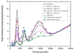
Figure 4. The total thermal conductivity of CO2–CH4 plasmas with different molar proportions under LTE. The results of Aubreton et al [39] and Yang et al [10] are shown with symbols for comparison.
Download figure:
Standard image High-resolution imageThe influence of mixture ratio on viscosity under LTE is shown in figure 5. Due to the positive correlation between molar weight and viscosity, the increase of CO2 proportion in CO2–CH4 mixture significantly increases the viscosity especially in low temperature. Our results of pure CO2 show good agreement with Yang et al [10] while our results of 50% CO2–50%CH4 is slightly lower than that of Aubreton [39]. This may be also due to the different use of polarizability.
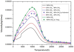
Figure 5. Temperature dependence of the viscosity of CO2–CH4 plasmas with different molar proportions under LTE.
Download figure:
Standard image High-resolution imageAnother phenomenon shown in viscosity of pure CH4 in figure 5 should be noted. Due to the reaction CH4 ↔ 2H2 + C(c), the transport process is dominated by gaseous H2 and H in temperature range from 1200 to 4100 K, since the condensed graphite does not contribute to the transport process. Due to the low polarizability and low molar weight of H2 and H, the viscosity of pure CH4 lowers sharply in this temperature range. The slight fluctuation in viscosity of 20% CO2–80%CH4 is also caused by this reason.
As shown in figures 5 and 6, the presence of condensed phase can significantly influence the composition and further affect the transport coefficients, especially in the CO2–CH4 mixture with CH4 proportion higher than 50%. For the viscosity, the reaction CH4 ↔ 2H2 + C(c) causes sharp decrease in temperature from 1200 to 4100 K. This phenomenon is significant in pure CH4 system, in which the system is dominated by H2 in temperature from 1500 to 4000 K. The viscosity in this temperature range agrees well with that of pure H2 plasma presented by Capitelli et al [40]. For the total thermal conductivity, the presence of condensed phase increases the molar fraction of H2 and therefore increases its dissociation temperature. For the mixture with CH4 proportion lower than 50%, the influence of condensed phase is negligible at 1 atm under LTE. The influence of condensed phase on electrical conductivity is negligible because at this temperature range (lower than 4000 K) there are barely electrons and ions in system and therefore the electrical conductivity is relatively low. Therefore the comparison is not presented.
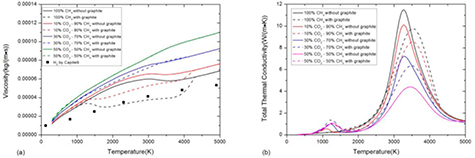
Figure 6. Influence of considering condensed phase in CO2–CH4 mixture with different ratio at atmospheric pressure under LTE on (a) viscosity and (b) total thermal conductivity. The viscosity of H2 presented by Capitelli is also presented for comparison [40]. Reproduced with permission from [40]. Copyright 1977 EDP Sciences.
Download figure:
Standard image High-resolution image3.2. Influence of non-equilibrium parameter
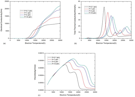
In a two-temperature CO2–CH4 mixture, the non-LTE effect may significantly affect both the dissociation and ionization process and further affect the thermo-physical properties. For the electrical conductivity, see figure 7(a), the delay of dissociation reactions in non-LTE system limits the number density of monatomic species at low electron temperature [41, 42]. Therefore the increase of non-equilibrium parameter θ decreases the electrical conductivity at low temperature. Once the dissociation reaction occurs, the ionization can be extremely rapid due to the high electron temperature, which causes the sharp increase in electrical conductivity.
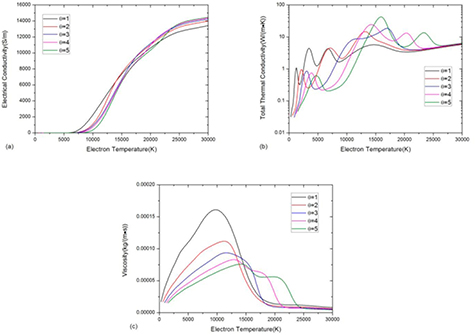
Figure 7. Transport coefficients of 50%CO2–50%CH4 mixture against electron temperature at atmospheric pressure with different non-equilibrium parameter θ (a) electrical conductivity, (b) thermal conductivity and (c) viscosity.
Download figure:
Standard image High-resolution imageThe delay of dissociation reactions in non-LTE system can significantly affect the total thermal conductivity mainly by influence the reactive thermal conductivity. Under LTE, the first peak at 1200 K is due to the phase transition and reaction CO2 + CH4 ↔ 2CO + 2H2. The other peaks at 3200 K, 6800 K and 15 000 K are due to H2 dissociation, CO dissociation and first order ionization respectively. For θ = 3, as shown in blue curve in figure 7(b), the first peak due to CO2 + CH4 ↔ 2CO + 2H2 reaction is shifted to Te = 3000 K. The gentle peak at around Te = 12 000 K is due to the combination of H2 dissociation at 10 000 K and H ionization at 14 000 K. Besides, the CO dissociation reactions are shifted to higher electron temperature, higher than that required for C and O ionization reactions. Once CO dissociation takes place, the ionization of C and O occur at the same time, which leads to a sharp peak at Te = 17 000 K. As the degree of non-equilibrium increases further (see the θ = 5 curve), the electron temperature at which H2 dissociates is higher than that of H ionization. It leads to a sharp peak at Te = 16 000 K rather than a gentle peak shown in θ = 3 curve.
The non-LTE effect can also affect the viscosity, as shown in figure 7(c). As given in equation (6), the viscosity is proportional to  . At same Te, as the increase of θ, the
  decreases therefore the viscosity is limited to a lower value. Ionization is also delayed, as discussed above, nevertheless the peak value of viscosity that is reached before ionization is much lower than for the LTE case. Besides, when θ is higher than 4, the high dissociation temperature of CO leads to a stepwise decrease in viscosity.
On the other hand, from the perspective of Th, the influence of non-LTE effect on thermal conductivity can be different or even opposite, as shown in figure 8. In non-LTE system, the high electron temperature promotes the ionization of dissociation product and therefore promotes the dissociation process. For instance, the reaction CO ↔ C + O occurs at 6800 K at LTE system, while in non-LTE system this reaction is shifted to Th = 5700 K when θ = 3 and Th = 4600 K when θ = 5. This is because the ionization of C and O consumes the dissociation product and further promotes the dissociation process. As a result, the peaks in thermal conductivity caused by CO dissociation are shifted to lower Th in non-LTE system. For H2 dissociation, this phenomenon occurs only when θ ⩾ 5, due to its relatively low dissociation temperature where the ionization of H does not occur in low θ system.
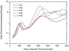
Figure 8. Total thermal conductivity of 50%CO2–50%CH4 mixture against heavy species temperature at atmospheric pressure with different non-equilibrium parameter θ.
Download figure:
Standard image High-resolution imageAs shown in the first article [5], the molar fraction of graphite decreases as non-equilibrium parameter increases no matter from the Te scale or Th scale. Therefore, the influence of condensed phase species, which is closely related to the condensed species composition, is negligible in high non-LTE system, see figure 9. For the non-LTE system whose θ is higher than 3, the molar fraction of graphite is too small to make difference in thermal conductivity.
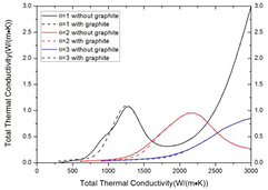
Figure 9. Influence of considering condensed phase in 2-T 50%CO2–50%CH4 mixture at atmospheric pressure on total thermal conductivity.
Download figure:
Standard image High-resolution image3.3. Influence of mixture ratio in 2-T system
In a non-LTE system, due to the delay of dissociation reactions which may change the sequence of reactions, the influence of mixture ratio is different with that in LTE system. For the electrical conductivity, the difference can be found in low temperature range. Under LTE system, the low ionization temperature of C makes C+ dominates the system ionization in low temperature. However, in non-LTE system, the delay of CO dissociation leads to low proportion of C atom and therefore limits the C ionization. On the other hand, the early dissociation of H2 makes H the only monatomic species in low temperature. Therefore in non-LTE system, the ionization process at low temperature is dominated by H+. As a consequence, in 2-T system, the electrical conductivity increases as the CH4 ratio in whole temperature range, as shown in figure 10(a). Besides, a sharp increase at around 24 000 K can be found in pure CO2 and CO2–CH4 mixture, which is due to the dissociation of CO and ionization of C and O atom.
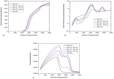
Figure 10. Transport coefficients of CO2–CH4 mixture at atmospheric pressure with θ = 5 and different non-equilibrium parameter (a) electrical conductivity, (b) thermal conductivity and (c) viscosity.
Download figure:
Standard image High-resolution imageIn non-LTE system, the delay of dissociation reaction makes dissociation and ionization reactions occur at same temperature and leads to high peaks in thermal conductivity. As shown in figure 10(b), the first peak, which can only be found in CO2–CH4 mixture, is due to the dissociation of H2O. The peak at around 14 000 K in high CH4-content system is due to the successive dissociation of CH4. The peaks at around 16 000 K and 23 000 K are respectively caused by H2 and CO dissociation. The largest peak can be found in 50%CO2–50%CH4 mixture due to the high molar fraction of H2 caused by reaction CO2 + CH4 ↔ 2CO + 2H2.
Similar to the LTE system, the viscosity in non-LTE CO2–CH4 system increases as CO2 proportion, as shown in figure 10(c). Besides, the stepwise decrease caused by high dissociation temperature of CO dissociation can be found in pure CO2 and CO2–CH4 mixture.
The influence of condensed phase in non-LTE CO2–CH4 mixture is much weaker than that in LTE system due to the low molar fraction of graphite [5], as shown in figure 11. The slight difference between multiphase system and pure gaseous system can be found in pure CH4 system as shown in black solid and dashed curve in figure 11. For CO2–CH4 mixture and pure CO2 system, the multiphase effect is negligible in non-LTE assumption.
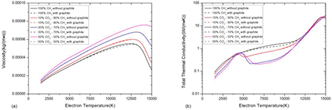
Figure 11. Influence of considering condensed phase in CO2–CH4 mixture with different ratio at atmospheric pressure with θ = 5 on (a) viscosity and (b) total thermal conductivity.
Download figure:
Standard image High-resolution image3.4. Influence of pressure in LTE and 2-T system
Figure 12 shows the influence of pressure on the specific heat and transport coefficients for pressures 0.1 atm, 1 atm, 5 atm and 10 atm for θ = 5. According to Le Chatelier's law, the increase of the pressure opposes changes to the original state of equilibrium, so that dissociation and ionization reactions are shifted to higher electron temperature as the pressure increases. As a result, the sharp increase in electrical conductivity and peaks in thermal conductivity and viscosity are shifted to higher electron temperature in high pressure system.
Figure 12. Temperature dependence of thermodynamic and transport properties, (a) electrical conductivity, (b) total thermal conductivity and (c) viscosity of 50%CO2–50%CH4 and θ = 5 at different pressures.
Download figure:
Standard image High-resolution image
4. Conclusion
In this paper, the transport coefficients of CO2–CH4 are calculated under LTE and non-LTE assumption. The multiphase effect is taken into account by using the composition results considering the graphite, which is presented in the first paper in this series [5], while the contribution of condensed species to transport process is neglected. The classical Chapman–Enskog method simplified by Devoto is applied in the present calculation with the newest interaction potential model and data. The results are presented for electron temperatures from 300 to 30 000 K, pressures from 0.1 to 10 atm and non-equilibrium parameter from 1 to 5. These results can be used to research the influence of condensed species on LTE and non-LTE plasma and can be served as reliable reference data for computational simulation of the behavior of CO2–CH4 plasmas. Some of the calculation results are tabulated in appendix in tables A1–A4.
The influence of condensed phase on transport coefficients is significant especially in high CH4-content system under LTE assumption due to the production of graphite during the CH4 dissociation. The multiphase effect leads to high H2 proportion in system and therefore causes a sharp decrease in viscosity. Besides, the total thermal conductivity which is sensitive to reactions is also affected by the condensed species. However, in non-LTE system, the influence of condensed phase is basically negligible due to the low molar fraction of graphite.
The influence of mixture ratio on transport coefficients of 2-T CO2–CH4 mixture is different with that on LTE system, mainly due to the different reaction sequence in non-LTE system. Unlike the LTE CO2–CH4 mixture in which the ionization process in low temperature is dominated by C+, the initial ionization of non-LTE CO2–CH4 mixture is dominated by H ionization due to the high dissociation temperature of CO. Therefore in 2-T system, the electrical conductivity increases as the CH4 ratio in whole temperature range. Besides, the temperature difference between H2 and CO dissociation leads to a stepwise decrease in the viscosity of CO2–CH4 and pure CO2 system under non-LTE condition. Besides, as the increase of pressure, the reactions are shifted to higher temperature according to Le Chatelier's law.
Acknowledgment
This work is supported by the National Key Basic Research Program of China (973 Program, No. 2015CB251002), the National Natural Science Foundation of China (No. 51521065, 51577145, 51377128).
Appendix.: Tabular transport coefficients
Table A1. Transport coefficients of CO2–CH4 mixture at atmospheric pressure under LTE.
| Te (K) | 20%CO2–80%CH4 | 50%CO2–50%CH4 | 80%CO2–20%CH4 | ||||||
|---|---|---|---|---|---|---|---|---|---|
| λtot (W/m/K) | μ (kg/m/s) | σ (S m−1) | λtot (W/m/K) | μ (kg/m/s) | σ (S m−1) | λtot (W/m/K) | μ (kg/m/s) | σ (S m−1) | |
| 300 | 2.42 × 10−02 | 1.39 × 10−05 | 7.47 × 10⁻¹¹ | 3.14 × 10−02 | 1.71 × 10−05 | 8.68 × 10⁻¹¹ | 2.29 × 10−02 | 1.80 × 10−05 | 7.32 × 10⁻¹¹ |
| 400 | 3.93 × 10−02 | 1.76 × 10−05 | 9.96 × 10⁻¹¹ | 4.38 × 10−02 | 2.13 × 10−05 | 1.14 × 10⁻¹⁰ | 3.10 × 10−02 | 2.30 × 10−05 | 9.76 × 10⁻¹¹ |
| 600 | 6.96 × 10−02 | 2.39 × 10−05 | 1.49 × 10⁻¹⁰ | 6.60 × 10−02 | 2.87 × 10−05 | 1.66 × 10⁻¹⁰ | 4.72 × 10−02 | 3.18 × 10−05 | 1.46 × 10⁻¹⁰ |
| 800 | 1.55 × 10−01 | 2.91 × 10−05 | 1.99 × 10⁻¹⁰ | 1.33 × 10−01 | 3.48 × 10−05 | 2.17 × 10⁻¹⁰ | 1.05 × 10−01 | 3.90 × 10−05 | 1.95 × 10⁻¹⁰ |
| 1000 | 5.80 × 10−01 | 3.41 × 10−05 | 2.54 × 10⁻¹⁰ | 5.19 × 10−01 | 4.03 × 10−05 | 2.70 × 10⁻¹⁰ | 2.94 × 10−01 | 4.52 × 10−05 | 2.49 × 10⁻¹⁰ |
| 1200 | 1.32 × 10−00 | 3.90 × 10−05 | 3.26 × 10⁻¹⁰ | 1.05 × 10−00 | 4.57 × 10−05 | 3.27 × 10⁻¹⁰ | 1.14 × 10−01 | 5.06 × 10−05 | 3.11 × 10⁻¹⁰ |
| 1400 | 9.67 × 10−01 | 4.23 × 10−05 | 4.28 × 10⁻¹⁰ | 8.72 × 10−01 | 5.04 × 10−05 | 4.09 × 10⁻¹⁰ | 8.86 × 10−02 | 5.64 × 10−05 | 3.63 × 10⁻¹⁰ |
| 1600 | 5.20 × 10−01 | 4.43 × 10−05 | 5.37 × 10⁻¹⁰ | 4.28 × 10−01 | 5.49 × 10−05 | 4.88 × 10⁻¹⁰ | 9.82 × 10−02 | 6.20 × 10−05 | 4.14 × 10⁻¹⁰ |
| 1800 | 4.78 × 10−01 | 4.69 × 10−05 | 6.27 × 10⁻¹⁰ | 3.17 × 10−01 | 5.94 × 10−05 | 5.55 × 10⁻¹⁰ | 1.10 × 10−01 | 6.73 × 10−05 | 4.66 × 10⁻¹⁰ |
| 2000 | 5.79 × 10−01 | 4.98 × 10−05 | 7.04 × 10⁻¹⁰ | 3.56 × 10−01 | 6.37 × 10−05 | 6.17 × 10⁻¹⁰ | 1.27 × 10−01 | 7.22 × 10−05 | 5.18 × 10⁻¹⁰ |
| 2200 | 8.10 × 10−01 | 5.28 × 10−05 | 7.74 × 10⁻¹⁰ | 5.02 × 10−01 | 6.77 × 10−05 | 6.78 × 10⁻¹⁰ | 1.58 × 10−01 | 7.69 × 10−05 | 5.69 × 10⁻¹⁰ |
| 2400 | 1.25 × 10−00 | 5.57 × 10−05 | 2.51 × 10−09 | 7.98 × 10−01 | 7.16 × 10−05 | 1.92 × 10−09 | 2.14 × 10−01 | 8.12 × 10−05 | 7.11 × 10⁻¹⁰ |
| 2600 | 2.01 × 10−00 | 5.85 × 10−05 | 5.54 × 10−08 | 1.31 × 10−00 | 7.53 × 10−05 | 4.09 × 10−08 | 3.24 × 10−01 | 8.54 × 10−05 | 1.52 × 10−08 |
| 2800 | 3.14 × 10−00 | 6.12 × 10−05 | 8.21 × 10−07 | 2.06 × 10−00 | 7.91 × 10−05 | 5.63 × 10−07 | 5.72 × 10−01 | 8.94 × 10−05 | 2.16 × 10−07 |
| 3000 | 4.61 × 10−00 | 6.37 × 10−05 | 8.89 × 10−06 | 3.00 × 10−00 | 8.30 × 10−05 | 5.39 × 10−06 | 1.15 × 10−00 | 9.34 × 10−05 | 2.26 × 10−06 |
| 3500 | 7.44 × 10−00 | 6.89 × 10−05 | 1.19 × 10−03 | 4.40 × 10−00 | 9.25 × 10−05 | 3.86 × 10−04 | 3.44 × 10−00 | 1.04 × 10−04 | 2.71 × 10−04 |
| 4000 | 4.45 × 10−00 | 7.29 × 10−05 | 5.41 × 10−02 | 2.65 × 10−00 | 9.93 × 10−05 | 8.07 × 10−03 | 1.95 × 10−00 | 1.14 × 10−04 | 7.61 × 10−03 |
| 4500 | 1.71 × 10−00 | 7.92 × 10−05 | 6.11 × 10−01 | 1.39 × 10−00 | 1.05 × 10−04 | 9.56 × 10−02 | 6.92 × 10−01 | 1.23 × 10−04 | 8.25 × 10−02 |
| 5000 | 1.19 × 10−00 | 8.42 × 10−05 | 2.80 × 10−00 | 1.28 × 10−00 | 1.10 × 10−04 | 7.66 × 10−01 | 5.37 × 10−01 | 1.31 × 10−04 | 5.58 × 10−01 |
| 5500 | 1.20 × 10−00 | 8.94 × 10−05 | 9.86 × 10−00 | 1.84 × 10−00 | 1.16 × 10−04 | 4.47 × 10−00 | 6.75 × 10−01 | 1.40 × 10−04 | 3.09 × 10−00 |
| 6000 | 1.77 × 10−00 | 9.49 × 10−05 | 2.85 × 10+01 | 2.95 × 10−00 | 1.23 × 10−04 | 1.98 × 10+01 | 1.47 × 10−00 | 1.48 × 10−04 | 1.65 × 10+01 |
| 6500 | 2.77 × 10−00 | 1.01 × 10−04 | 7.18 × 10+01 | 4.08 × 10−00 | 1.30 × 10−04 | 6.69 × 10+01 | 3.20 × 10−00 | 1.56 × 10−04 | 7.20 × 10+01 |
| 7000 | 2.83 × 10−00 | 1.07 × 10−04 | 1.59 × 10+02 | 4.08 × 10−00 | 1.37 × 10−04 | 1.74 × 10+02 | 4.19 × 10−00 | 1.64 × 10−04 | 2.17 × 10+02 |
| 8000 | 1.79 × 10−00 | 1.17 × 10−04 | 5.11 × 10+02 | 1.98 × 10−00 | 1.50 × 10−04 | 6.07 × 10+02 | 2.15 × 10−00 | 1.80 × 10−04 | 8.02 × 10+02 |
| 9000 | 1.96 × 10−00 | 1.23 × 10−04 | 1.13 × 10+03 | 1.71 × 10−00 | 1.59 × 10−04 | 1.31 × 10+03 | 1.45 × 10−00 | 1.91 × 10−04 | 1.65 × 10+03 |
| 10 000 | 2.63 × 10−00 | 1.22 × 10−04 | 1.99 × 10+03 | 2.23 × 10−00 | 1.61 × 10−04 | 2.23 × 10+03 | 1.78 × 10−00 | 1.95 × 10−04 | 2.64 × 10+03 |
| 11 000 | 3.57 × 10−00 | 1.14 × 10−04 | 3.00 × 10+03 | 3.05 × 10−00 | 1.55 × 10−04 | 3.26 × 10+03 | 2.36 × 10−00 | 1.90 × 10−04 | 3.68 × 10+03 |
| 12 000 | 4.67 × 10−00 | 1.00 × 10−04 | 4.10 × 10+03 | 3.99 × 10−00 | 1.41 × 10−04 | 4.33 × 10+03 | 2.99 × 10−00 | 1.74 × 10−04 | 4.70 × 10+03 |
| 13 000 | 5.74 × 10−00 | 8.23 × 10−05 | 5.21 × 10+03 | 4.89 × 10−00 | 1.19 × 10−04 | 5.39 × 10+03 | 3.55 × 10−00 | 1.45 × 10−04 | 5.68 × 10+03 |
| 14 000 | 6.46 × 10−00 | 6.31 × 10−05 | 6.27 × 10+03 | 5.52 × 10−00 | 9.18 × 10−05 | 6.40 × 10+03 | 3.95 × 10−00 | 1.09 × 10−04 | 6.60 × 10+03 |
| 15 000 | 6.48 × 10−00 | 4.53 × 10−05 | 7.24 × 10+03 | 5.66 × 10−00 | 6.44 × 10−05 | 7.33 × 10+03 | 4.09 × 10−00 | 7.42 × 10−05 | 7.45 × 10+03 |
| 16 000 | 5.79 × 10−00 | 3.12 × 10−05 | 8.09 × 10+03 | 5.25 × 10−00 | 4.28 × 10−05 | 8.14 × 10+03 | 3.96 × 10−00 | 4.83 × 10−05 | 8.21 × 10+03 |
| 17 000 | 4.84 × 10−00 | 2.15 × 10−05 | 8.81 × 10+03 | 4.57 × 10−00 | 2.86 × 10−05 | 8.84 × 10+03 | 3.67 × 10−00 | 3.22 × 10−05 | 8.88 × 10+03 |
| 18 000 | 4.06 × 10−00 | 1.57 × 10−05 | 9.46 × 10+03 | 3.95 × 10−00 | 2.04 × 10−05 | 9.48 × 10+03 | 3.39 × 10−00 | 2.31 × 10−05 | 9.50 × 10+03 |
| 19 000 | 3.60 × 10−00 | 1.25 × 10−05 | 1.01 × 10+04 | 3.55 × 10−00 | 1.61 × 10−05 | 1.01 × 10+04 | 3.23 × 10−00 | 1.84 × 10−05 | 1.01 × 10+04 |
| 20 000 | 3.41 × 10−00 | 1.09 × 10−05 | 1.06 × 10+04 | 3.38 × 10−00 | 1.39 × 10−05 | 1.06 × 10+04 | 3.19 × 10−00 | 1.60 × 10−05 | 1.06 × 10+04 |
| 22 000 | 3.54 × 10−00 | 9.83 × 10−06 | 1.16 × 10+04 | 3.52 × 10−00 | 1.25 × 10−05 | 1.16 × 10+04 | 3.44 × 10−00 | 1.47 × 10−05 | 1.16 × 10+04 |
| 24 000 | 4.00 × 10−00 | 9.47 × 10−06 | 1.25 × 10+04 | 3.97 × 10−00 | 1.20 × 10−05 | 1.24 × 10+04 | 3.91 × 10−00 | 1.42 × 10−05 | 1.23 × 10+04 |
| 26 000 | 4.59 × 10−00 | 8.65 × 10−06 | 1.30 × 10+04 | 4.55 × 10−00 | 1.10 × 10−05 | 1.28 × 10+04 | 4.48 × 10−00 | 1.30 × 10−05 | 1.26 × 10+04 |
| 28 000 | 5.21 × 10−00 | 7.64 × 10−06 | 1.34 × 10+04 | 5.15 × 10−00 | 9.51 × 10−06 | 1.31 × 10+04 | 5.06 × 10−00 | 1.11 × 10−05 | 1.28 × 10+04 |
| 30 000 | 5.85 × 10−00 | 6.90 × 10−06 | 1.39 × 10+04 | 5.77 × 10−00 | 8.14 × 10−06 | 1.34 × 10+04 | 5.66 × 10−00 | 9.10 × 10−06 | 1.29 × 10+04 |
Table A2. Transport Coefficients of CO2–CH4 mixture at atmospheric pressure with θ = 5.
| Te (K) | 20%CO2–80%CH4 | 50%CO2–50%CH4 | 80%CO2–20%CH4 | ||||||
|---|---|---|---|---|---|---|---|---|---|
| λtot (W/m/K) | μ (kg/m/s) | σ (S m−1) | λtot (W/m/K) | μ (kg/m/s) | σ (S m−1) | λtot (W/m/K) | μ (kg/m/s) | σ (S m−1) | |
| 1500 | 6.36 × 10−02 | 1.35 × 10−05 | 3.01 × 10⁻¹¹ | 4.67 × 10−02 | 1.54 × 10−05 | 2.99 × 10⁻¹¹ | 5.18 × 10−02 | 1.69 × 10−05 | 2.96 × 10⁻¹¹ |
| 1600 | 7.10 × 10−02 | 1.43 × 10−05 | 3.21 × 10⁻¹¹ | 5.16 × 10−02 | 1.63 × 10−05 | 3.19 × 10⁻¹¹ | 5.71 × 10−02 | 1.79 × 10−05 | 3.16 × 10⁻¹¹ |
| 1800 | 8.58 × 10−02 | 1.58 × 10−05 | 3.62 × 10⁻¹¹ | 6.14 × 10−02 | 1.81 × 10−05 | 3.58 × 10⁻¹¹ | 6.76 × 10−02 | 2.00 × 10−05 | 3.55 × 10⁻¹¹ |
| 2000 | 1.02 × 10−01 | 1.74 × 10−05 | 4.02 × 10⁻¹¹ | 7.19 × 10−02 | 1.99 × 10−05 | 3.98 × 10⁻¹¹ | 7.84 × 10−02 | 2.20 × 10−05 | 3.95 × 10⁻¹¹ |
| 2200 | 1.21 × 10−01 | 1.88 × 10−05 | 4.42 × 10⁻¹¹ | 8.34 × 10−02 | 2.16 × 10−05 | 4.38 × 10⁻¹¹ | 8.98 × 10−02 | 2.39 × 10−05 | 4.34 × 10⁻¹¹ |
| 2400 | 1.42 × 10−01 | 2.02 × 10−05 | 4.82 × 10⁻¹¹ | 9.69 × 10−02 | 2.33 × 10−05 | 4.78 × 10⁻¹¹ | 1.03 × 10−01 | 2.58 × 10−05 | 4.74 × 10⁻¹¹ |
| 2600 | 1.67 × 10−01 | 2.16 × 10−05 | 5.22 × 10⁻¹¹ | 1.14 × 10−01 | 2.49 × 10−05 | 5.18 × 10⁻¹¹ | 1.18 × 10−01 | 2.76 × 10−05 | 5.13 × 10⁻¹¹ |
| 2800 | 1.96 × 10−01 | 2.29 × 10−05 | 5.63 × 10⁻¹¹ | 1.35 × 10−01 | 2.64 × 10−05 | 5.58 × 10⁻¹¹ | 1.37 × 10−01 | 2.93 × 10−05 | 5.53 × 10⁻¹¹ |
| 3000 | 2.33 × 10−01 | 2.41 × 10−05 | 6.04 × 10⁻¹¹ | 1.63 × 10−01 | 2.79 × 10−05 | 5.99 × 10⁻¹¹ | 1.63 × 10−01 | 3.09 × 10−05 | 5.94 × 10⁻¹¹ |
| 3200 | 2.78 × 10−01 | 2.52 × 10−05 | 6.46 × 10⁻¹¹ | 2.02 × 10−01 | 2.92 × 10−05 | 6.42 × 10⁻¹¹ | 1.96 × 10−01 | 3.25 × 10−05 | 6.37 × 10⁻¹¹ |
| 3400 | 3.34 × 10−01 | 2.63 × 10−05 | 6.91 × 10⁻¹¹ | 2.52 × 10−01 | 3.06 × 10−05 | 6.87 × 10⁻¹¹ | 2.40 × 10−01 | 3.40 × 10−05 | 6.82 × 10⁻¹¹ |
| 3600 | 3.99 × 10−01 | 2.75 × 10−05 | 7.37 × 10⁻¹¹ | 3.14 × 10−01 | 3.19 × 10−05 | 7.37 × 10⁻¹¹ | 2.87 × 10−01 | 3.54 × 10−05 | 7.31 × 10⁻¹¹ |
| 3800 | 4.72 × 10−01 | 2.86 × 10−05 | 2.32 × 10⁻¹⁰ | 3.86 × 10−01 | 3.32 × 10−05 | 2.25 × 10⁻¹⁰ | 3.39 × 10−01 | 3.69 × 10−05 | 2.05 × 10⁻¹⁰ |
| 4000 | 5.44 × 10−01 | 2.97 × 10−05 | 1.97 × 10−09 | 4.54 × 10−01 | 3.44 × 10−05 | 1.92 × 10−09 | 3.71 × 10−01 | 3.82 × 10−05 | 1.73 × 10−09 |
| 4500 | 6.45 × 10−01 | 3.24 × 10−05 | 1.81 × 10−07 | 5.95 × 10−01 | 3.74 × 10−05 | 1.81 × 10−07 | 3.29 × 10−01 | 4.14 × 10−05 | 1.54 × 10−07 |
| 5000 | 4.52 × 10−01 | 3.48 × 10−05 | 6.41 × 10−06 | 5.78 × 10−01 | 4.00 × 10−05 | 6.85 × 10−06 | 1.11 × 10−01 | 4.45 × 10−05 | 4.88 × 10−06 |
| 5500 | 2.93 × 10−01 | 3.72 × 10−05 | 1.08 × 10−04 | 3.96 × 10−01 | 4.25 × 10−05 | 1.28 × 10−04 | 8.70 × 10−02 | 4.76 × 10−05 | 7.51 × 10−05 |
| 6000 | 3.00 × 10−01 | 3.97 × 10−05 | 1.10 × 10−03 | 2.52 × 10−01 | 4.49 × 10−05 | 1.40 × 10−03 | 9.23 × 10−02 | 5.07 × 10−05 | 7.33 × 10−04 |
| 6500 | 3.27 × 10−01 | 4.21 × 10−05 | 7.90 × 10−03 | 2.08 × 10−01 | 4.74 × 10−05 | 1.03 × 10−02 | 1.00 × 10−01 | 5.36 × 10−05 | 5.08 × 10−03 |
| 7000 | 3.55 × 10−01 | 4.44 × 10−05 | 4.31 × 10−02 | 2.05 × 10−01 | 4.99 × 10−05 | 5.70 × 10−02 | 1.09 × 10−01 | 5.65 × 10−05 | 2.70 × 10−02 |
| 8000 | 4.17 × 10−01 | 4.89 × 10−05 | 6.94 × 10−01 | 2.34 × 10−01 | 5.47 × 10−05 | 9.23 × 10−01 | 1.30 × 10−01 | 6.21 × 10−05 | 4.15 × 10−01 |
| 9000 | 5.05 × 10−01 | 5.31 × 10−05 | 6.14 × 10−00 | 2.98 × 10−01 | 5.93 × 10−05 | 8.16 × 10−00 | 1.63 × 10−01 | 6.73 × 10−05 | 3.55 × 10−00 |
| 10 000 | 6.93 × 10−01 | 5.69 × 10−05 | 3.55 × 10+01 | 4.78 × 10−01 | 6.36 × 10−05 | 4.68 × 10+01 | 2.41 × 10−01 | 7.23 × 10−05 | 2.00 × 10+01 |
| 11 000 | 1.17 × 10−00 | 6.03 × 10−05 | 1.50 × 10+02 | 1.02 × 10−00 | 6.76 × 10−05 | 1.91 × 10+02 | 4.52 × 10−01 | 7.69 × 10−05 | 8.24 × 10+01 |
| 12 000 | 2.40 × 10−00 | 6.30 × 10−05 | 5.08 × 10+02 | 2.48 × 10−00 | 7.13 × 10−05 | 5.92 × 10+02 | 9.88 × 10−01 | 8.12 × 10−05 | 2.65 × 10+02 |
| 13 000 | 5.99 × 10−00 | 6.42 × 10−05 | 1.56 × 10+03 | 6.01 × 10−00 | 7.43 × 10−05 | 1.44 × 10+03 | 2.23 × 10−00 | 8.51 × 10−05 | 7.03 × 10+02 |
| 14 000 | 1.60 × 10+01 | 5.89 × 10−05 | 3.97 × 10+03 | 1.38 × 10+01 | 7.59 × 10−05 | 2.90 × 10+03 | 5.09 × 10−00 | 8.81 × 10−05 | 1.65 × 10+03 |
| 15 000 | 2.39 × 10+01 | 4.28 × 10−05 | 6.45 × 10+03 | 2.92 × 10+01 | 7.38 × 10−05 | 4.90 × 10+03 | 1.17 × 10+01 | 8.89 × 10−05 | 3.45 × 10+03 |
| 16 000 | 3.07 × 10+01 | 2.96 × 10−05 | 7.97 × 10+03 | 4.22 × 10+01 | 6.48 × 10−05 | 6.94 × 10+03 | 2.25 × 10+01 | 8.16 × 10−05 | 6.02 × 10+03 |
| 17 000 | 2.12 × 10+01 | 2.18 × 10−05 | 9.04 × 10+03 | 2.26 × 10+01 | 5.71 × 10−05 | 8.28 × 10+03 | 1.57 × 10+01 | 6.61 × 10−05 | 7.88 × 10+03 |
| 18 000 | 9.51 × 10−00 | 1.96 × 10−05 | 9.82 × 10+03 | 9.08 × 10−00 | 5.55 × 10−05 | 9.10 × 10+03 | 7.40 × 10−00 | 5.94 × 10−05 | 8.77 × 10+03 |
| 19 000 | 5.78 × 10−00 | 1.93 × 10−05 | 1.05 × 10+04 | 5.60 × 10−00 | 5.60 × 10−05 | 9.74 × 10+03 | 5.00 × 10−00 | 5.81 × 10−05 | 9.39 × 10+03 |
| 20 000 | 4.59 × 10−00 | 1.96 × 10−05 | 1.11 × 10+04 | 4.91 × 10−00 | 5.61 × 10−05 | 1.03 × 10+04 | 4.17 × 10−00 | 5.87 × 10−05 | 9.93 × 10+03 |
| 22 000 | 5.26 × 10−00 | 1.81 × 10−05 | 1.22 × 10+04 | 8.57 × 10−00 | 4.24 × 10−05 | 1.17 × 10+04 | 6.39 × 10−00 | 5.54 × 10−05 | 1.11 × 10+04 |
| 24 000 | 7.05 × 10−00 | 6.53 × 10−06 | 1.34 × 10+04 | 1.15 × 10+01 | 1.09 × 10−05 | 1.33 × 10+04 | 1.56 × 10+01 | 1.57 × 10−05 | 1.31 × 10+04 |
| 26 000 | 5.19 × 10−00 | 4.63 × 10−06 | 1.41 × 10+04 | 5.42 × 10−00 | 5.97 × 10−06 | 1.39 × 10+04 | 5.66 × 10−00 | 7.17 × 10−06 | 1.37 × 10+04 |
| 28 000 | 5.72 × 10−00 | 4.11 × 10−06 | 1.45 × 10+04 | 5.70 × 10−00 | 5.15 × 10−06 | 1.42 × 10+04 | 5.64 × 10−00 | 6.03 × 10−06 | 1.39 × 10+04 |
| 30 000 | 6.39 × 10−00 | 3.66 × 10−06 | 1.49 × 10+04 | 6.36 × 10−00 | 4.42 × 10−06 | 1.45 × 10+04 | 6.30 × 10−00 | 5.00 × 10−06 | 1.39 × 10+04 |
Table A3. Transport Coefficients of 50%CO2–50%CH4 mixture under LTE at different pressure.
| Te (K) | 0.1 atm | 5 atm | 10 atm | ||||||
|---|---|---|---|---|---|---|---|---|---|
| λtot (W/m/K) | μ (kg/m/s) | σ (S m−1) | λtot (W/m/K) | μ (kg/m/s) | σ (S m−1) | λtot (W/m/K) | μ (kg/m/s) | σ (S m−1) | |
| 300 | 1.50 × 10−02 | 1.67 × 10−05 | 7.91 × 10⁻¹⁰ | 4.35 × 10−02 | 1.72 × 10−05 | 1.76 × 10⁻¹¹ | 4.37 × 10−02 | 1.72 × 10−05 | 8.81 × 10⁻¹² |
| 400 | 2.75 × 10−02 | 2.07 × 10−05 | 1.00 × 10−09 | 5.46 × 10−02 | 2.14 × 10−05 | 2.34 × 10⁻¹¹ | 5.54 × 10−02 | 2.14 × 10−05 | 1.17 × 10⁻¹¹ |
| 600 | 5.24 × 10−02 | 2.82 × 10−05 | 1.44 × 10−09 | 7.69 × 10−02 | 2.88 × 10−05 | 3.48 × 10⁻¹¹ | 7.88 × 10−02 | 2.88 × 10−05 | 1.75 × 10⁻¹¹ |
| 800 | 3.85 × 10−01 | 3.45 × 10−05 | 1.90 × 10−09 | 1.15 × 10−01 | 3.48 × 10−05 | 4.61 × 10⁻¹¹ | 1.12 × 10−01 | 3.48 × 10−05 | 2.33 × 10⁻¹¹ |
| 1000 | 9.79 × 10−01 | 4.02 × 10−05 | 2.59 × 10−09 | 2.53 × 10−01 | 4.00 × 10−05 | 5.76 × 10⁻¹¹ | 2.02 × 10−01 | 3.99 × 10−05 | 2.91 × 10⁻¹¹ |
| 1200 | 1.02 × 10−00 | 4.52 × 10−05 | 3.50 × 10−09 | 5.46 × 10−01 | 4.51 × 10−05 | 6.94 × 10⁻¹¹ | 3.56 × 10−01 | 4.49 × 10−05 | 3.51 × 10⁻¹¹ |
| 1400 | 3.52 × 10−01 | 4.99 × 10−05 | 4.30 × 10−09 | 7.19 × 10−01 | 5.04 × 10−05 | 8.23 × 10⁻¹¹ | 4.42 × 10−01 | 5.00 × 10−05 | 4.14 × 10⁻¹¹ |
| 1600 | 2.59 × 10−01 | 5.47 × 10−05 | 4.94 × 10−09 | 5.79 × 10−01 | 5.52 × 10−05 | 9.65 × 10⁻¹¹ | 4.24 × 10−01 | 5.51 × 10−05 | 4.81 × 10⁻¹¹ |
| 1800 | 3.14 × 10−01 | 5.93 × 10−05 | 5.57 × 10−09 | 4.01 × 10−01 | 5.95 × 10−05 | 1.10 × 10⁻¹⁰ | 3.57 × 10−01 | 5.97 × 10−05 | 5.49 × 10⁻¹¹ |
| 2000 | 4.97 × 10−01 | 6.37 × 10−05 | 6.17 × 10−09 | 3.54 × 10−01 | 6.38 × 10−05 | 1.23 × 10⁻¹⁰ | 3.36 × 10−01 | 6.39 × 10−05 | 6.15 × 10⁻¹¹ |
| 2200 | 9.30 × 10−01 | 6.77 × 10−05 | 6.71 × 10−09 | 4.04 × 10−01 | 6.78 × 10−05 | 1.36 × 10⁻¹⁰ | 3.74 × 10−01 | 6.78 × 10−05 | 6.78 × 10⁻¹¹ |
| 2400 | 1.77 × 10−00 | 7.17 × 10−05 | 1.07 × 10−08 | 5.39 × 10−01 | 7.16 × 10−05 | 5.72 × 10⁻¹⁰ | 4.74 × 10−01 | 7.16 × 10−05 | 3.39 × 10⁻¹⁰ |
| 2600 | 3.05 × 10−00 | 7.56 × 10−05 | 2.23 × 10−07 | 7.85 × 10−01 | 7.53 × 10−05 | 1.22 × 10−08 | 6.54 × 10−01 | 7.53 × 10−05 | 7.21 × 10−09 |
| 2800 | 4.46 × 10−00 | 7.97 × 10−05 | 2.85 × 10−06 | 1.17 × 10−00 | 7.89 × 10−05 | 1.68 × 10−07 | 9.37 × 10−01 | 7.89 × 10−05 | 9.92 × 10−08 |
| 3000 | 5.13 × 10−00 | 8.38 × 10−05 | 2.29 × 10−05 | 1.70 × 10−00 | 8.26 × 10−05 | 1.65 × 10−06 | 1.34 × 10−00 | 8.25 × 10−05 | 9.60 × 10−07 |
| 3500 | 2.41 × 10−00 | 9.23 × 10−05 | 1.29 × 10−03 | 3.37 × 10−00 | 9.21 × 10−05 | 1.51 × 10−04 | 2.75 × 10−00 | 9.19 × 10−05 | 8.94 × 10−05 |
| 4000 | 1.03 × 10−00 | 9.88 × 10−05 | 3.05 × 10−02 | 3.86 × 10−00 | 1.00 × 10−04 | 3.48 × 10−03 | 3.75 × 10−00 | 1.00 × 10−04 | 2.41 × 10−03 |
| 4500 | 1.07 × 10−00 | 1.04 × 10−04 | 4.18 × 10−01 | 2.60 × 10−00 | 1.06 × 10−04 | 3.78 × 10−02 | 3.17 × 10−00 | 1.06 × 10−04 | 2.61 × 10−02 |
| 5000 | 1.82 × 10−00 | 1.10 × 10−04 | 3.69 × 10−00 | 1.66 × 10−00 | 1.11 × 10−04 | 2.78 × 10−01 | 2.10 × 10−00 | 1.11 × 10−04 | 1.85 × 10−01 |
| 5500 | 3.38 × 10−00 | 1.16 × 10−04 | 2.19 × 10+01 | 1.55 × 10−00 | 1.16 × 10−04 | 1.53 × 10−00 | 1.66 × 10−00 | 1.17 × 10−04 | 9.86 × 10−01 |
| 6000 | 4.67 × 10−00 | 1.23 × 10−04 | 8.80 × 10+01 | 2.03 × 10−00 | 1.23 × 10−04 | 6.62 × 10−00 | 1.85 × 10−00 | 1.23 × 10−04 | 4.18 × 10−00 |
| 6500 | 3.66 × 10−00 | 1.31 × 10−04 | 2.39 × 10+02 | 2.91 × 10−00 | 1.30 × 10−04 | 2.32 × 10+01 | 2.49 × 10−00 | 1.30 × 10−04 | 1.46 × 10+01 |
| 7000 | 2.08 × 10−00 | 1.37 × 10−04 | 4.76 × 10+02 | 3.78 × 10−00 | 1.37 × 10−04 | 6.65 × 10+01 | 3.33 × 10−00 | 1.37 × 10−04 | 4.24 × 10+01 |
| 8000 | 1.60 × 10−00 | 1.45 × 10−04 | 1.15 × 10+03 | 3.24 × 10−00 | 1.50 × 10−04 | 3.10 × 10+02 | 3.68 × 10−00 | 1.50 × 10−04 | 2.17 × 10+02 |
| 9000 | 2.26 × 10−00 | 1.42 × 10−04 | 1.95 × 10+03 | 1.89 × 10−00 | 1.63 × 10−04 | 8.06 × 10+02 | 2.23 × 10−00 | 1.63 × 10−04 | 6.20 × 10+02 |
| 10 000 | 3.17 × 10−00 | 1.30 × 10−04 | 2.77 × 10+03 | 1.87 × 10−00 | 1.72 × 10−04 | 1.56 × 10+03 | 1.84 × 10−00 | 1.74 × 10−04 | 1.27 × 10+03 |
| 11 000 | 4.03 × 10−00 | 1.08 × 10−04 | 3.54 × 10+03 | 2.38 × 10−00 | 1.76 × 10−04 | 2.56 × 10+03 | 2.18 × 10−00 | 1.81 × 10−04 | 2.18 × 10+03 |
| 12 000 | 4.59 × 10−00 | 7.63 × 10−05 | 4.27 × 10+03 | 3.15 × 10−00 | 1.74 × 10−04 | 3.73 × 10+03 | 2.83 × 10−00 | 1.84 × 10−04 | 3.31 × 10+03 |
| 13 000 | 4.51 × 10−00 | 4.53 × 10−05 | 4.93 × 10+03 | 4.08 × 10−00 | 1.65 × 10−04 | 5.02 × 10+03 | 3.68 × 10−00 | 1.81 × 10−04 | 4.63 × 10+03 |
| 14 000 | 3.76 × 10−00 | 2.45 × 10−05 | 5.50 × 10+03 | 5.04 × 10−00 | 1.50 × 10−04 | 6.36 × 10+03 | 4.64 × 10−00 | 1.71 × 10−04 | 6.06 × 10+03 |
| 15 000 | 2.88 × 10−00 | 1.39 × 10−05 | 6.00 × 10+03 | 5.90 × 10−00 | 1.28 × 10−04 | 7.70 × 10+03 | 5.61 × 10−00 | 1.55 × 10−04 | 7.54 × 10+03 |
| 16 000 | 2.28 × 10−00 | 9.20 × 10−06 | 6.47 × 10+03 | 6.49 × 10−00 | 1.03 × 10−04 | 8.98 × 10+03 | 6.44 × 10−00 | 1.35 × 10−04 | 9.02 × 10+03 |
| 17 000 | 1.99 × 10−00 | 7.34 × 10−06 | 6.92 × 10+03 | 6.66 × 10−00 | 7.91 × 10−05 | 1.02 × 10+04 | 7.01 × 10−00 | 1.11 × 10−04 | 1.04 × 10+04 |
| 18 000 | 1.93 × 10−00 | 6.71 × 10−06 | 7.35 × 10+03 | 6.45 × 10−00 | 5.90 × 10−05 | 1.12 × 10+04 | 7.22 × 10−00 | 8.84 × 10−05 | 1.18 × 10+04 |
| 19 000 | 2.01 × 10−00 | 6.59 × 10−06 | 7.76 × 10+03 | 6.01 × 10−00 | 4.43 × 10−05 | 1.21 × 10+04 | 7.10 × 10−00 | 6.90 × 10−05 | 1.29 × 10+04 |
| 20 000 | 2.15 × 10−00 | 6.57 × 10−06 | 8.10 × 10+03 | 5.57 × 10−00 | 3.45 × 10−05 | 1.29 × 10+04 | 6.80 × 10−00 | 5.42 × 10−05 | 1.40 × 10+04 |
| 22 000 | 2.53 × 10−00 | 6.06 × 10−06 | 8.52 × 10+03 | 5.12 × 10−00 | 2.47 × 10−05 | 1.44 × 10+04 | 6.24 × 10−00 | 3.68 × 10−05 | 1.57 × 10+04 |
| 24 000 | 2.94 × 10−00 | 5.13 × 10−06 | 8.75 × 10+03 | 5.29 × 10−00 | 2.15 × 10−05 | 1.56 × 10+04 | 6.20 × 10−00 | 2.97 × 10−05 | 1.72 × 10+04 |
| 26 000 | 3.37 × 10−00 | 4.34 × 10−06 | 9.03 × 10+03 | 5.83 × 10−00 | 2.04 × 10−05 | 1.66 × 10+04 | 6.63 × 10−00 | 2.70 × 10−05 | 1.84 × 10+04 |
| 28 000 | 3.84 × 10−00 | 3.63 × 10−06 | 9.36 × 10+03 | 6.54 × 10−00 | 1.92 × 10−05 | 1.73 × 10+04 | 7.35 × 10−00 | 2.56 × 10−05 | 1.94 × 10+04 |
| 30 000 | 4.33 × 10−00 | 3.21 × 10−06 | 9.80 × 10+03 | 7.34 × 10−00 | 1.73 × 10−05 | 1.77 × 10+04 | 8.21 × 10−00 | 2.38 × 10−05 | 2.01 × 10+04 |
Table A4. Transport coefficients of 50%CO2–50%CH4 mixture at different pressure with θ = 5.
| Te (K) | 0.1 atm | 5 atm | 10 atm | ||||||
|---|---|---|---|---|---|---|---|---|---|
| λtot (W/m/K) | μ (kg/m/s) | σ (S m−1) | λtot (W/m/K) | μ (kg/m/s) | σ (S m−1) | λtot (W/m/K) | μ (kg/m/s) | σ (S m−1) | |
| 1500 | 4.68 × 10−02 | 1.54 × 10−05 | 2.99 × 10⁻¹⁰ | 4.62 × 10−02 | 1.54 × 10−05 | 5.99 × 10⁻¹² | 4.56 × 10−02 | 1.55 × 10−05 | 3.01 × 10⁻¹² |
| 1600 | 5.17 × 10−02 | 1.63 × 10−05 | 3.18 × 10⁻¹⁰ | 5.11 × 10−02 | 1.63 × 10−05 | 6.39 × 10⁻¹² | 5.06 × 10−02 | 1.64 × 10−05 | 3.20 × 10⁻¹² |
| 1800 | 6.15 × 10−02 | 1.81 × 10−05 | 3.58 × 10⁻¹⁰ | 6.09 × 10−02 | 1.81 × 10−05 | 7.18 × 10⁻¹² | 6.04 × 10−02 | 1.82 × 10−05 | 3.60 × 10⁻¹² |
| 2000 | 7.22 × 10−02 | 1.99 × 10−05 | 3.98 × 10⁻¹⁰ | 7.14 × 10−02 | 1.99 × 10−05 | 7.97 × 10⁻¹² | 7.09 × 10−02 | 1.99 × 10−05 | 3.99 × 10⁻¹² |
| 2200 | 8.47 × 10−02 | 2.16 × 10−05 | 4.38 × 10⁻¹⁰ | 8.27 × 10−02 | 2.17 × 10−05 | 8.77 × 10⁻¹² | 8.22 × 10−02 | 2.17 × 10−05 | 4.39 × 10⁻¹² |
| 2400 | 1.00 × 10−01 | 2.33 × 10−05 | 4.78 × 10⁻¹⁰ | 9.50 × 10−02 | 2.33 × 10−05 | 9.56 × 10⁻¹² | 9.43 × 10−02 | 2.33 × 10−05 | 4.79 × 10⁻¹² |
| 2600 | 1.23 × 10−01 | 2.49 × 10−05 | 5.18 × 10⁻¹⁰ | 1.09 × 10−01 | 2.49 × 10−05 | 1.04 × 10⁻¹¹ | 1.08 × 10−01 | 2.49 × 10−05 | 5.18 × 10⁻¹² |
| 2800 | 1.57 × 10−01 | 2.64 × 10−05 | 5.59 × 10⁻¹⁰ | 1.27 × 10−01 | 2.64 × 10−05 | 1.12 × 10⁻¹¹ | 1.23 × 10−01 | 2.64 × 10−05 | 5.58 × 10⁻¹² |
| 3000 | 2.12 × 10−01 | 2.79 × 10−05 | 6.02 × 10⁻¹⁰ | 1.49 × 10−01 | 2.79 × 10−05 | 1.20 × 10⁻¹¹ | 1.44 × 10−01 | 2.79 × 10−05 | 5.98 × 10⁻¹² |
| 3200 | 2.95 × 10−01 | 2.93 × 10−05 | 6.49 × 10⁻¹⁰ | 1.75 × 10−01 | 2.92 × 10−05 | 1.28 × 10⁻¹¹ | 1.68 × 10−01 | 2.92 × 10−05 | 6.39 × 10⁻¹² |
| 3400 | 4.11 × 10−01 | 3.06 × 10−05 | 7.02 × 10⁻¹⁰ | 2.08 × 10−01 | 3.06 × 10−05 | 1.37 × 10⁻¹¹ | 1.95 × 10−01 | 3.06 × 10−05 | 6.81 × 10⁻¹² |
| 3600 | 5.54 × 10−01 | 3.19 × 10−05 | 7.62 × 10⁻¹⁰ | 2.47 × 10−01 | 3.19 × 10−05 | 1.46 × 10⁻¹¹ | 2.32 × 10−01 | 3.19 × 10−05 | 7.25 × 10⁻¹² |
| 3800 | 7.02 × 10−01 | 3.32 × 10−05 | 1.88 × 10−09 | 2.90 × 10−01 | 3.31 × 10−05 | 5.11 × 10⁻¹¹ | 2.62 × 10−01 | 3.31 × 10−05 | 2.70 × 10⁻¹¹ |
| 4000 | 8.15 × 10−01 | 3.44 × 10−05 | 1.61 × 10−08 | 3.25 × 10−01 | 3.44 × 10−05 | 4.35 × 10⁻¹⁰ | 3.03 × 10−01 | 3.44 × 10−05 | 2.29 × 10⁻¹⁰ |
| 4500 | 7.29 × 10−01 | 3.70 × 10−05 | 1.45 × 10−06 | 4.07 × 10−01 | 3.74 × 10−05 | 4.10 × 10−08 | 3.84 × 10−01 | 3.75 × 10−05 | 2.16 × 10−08 |
| 5000 | 3.58 × 10−01 | 3.95 × 10−05 | 4.83 × 10−05 | 4.52 × 10−01 | 4.03 × 10−05 | 1.58 × 10−06 | 3.23 × 10−01 | 4.03 × 10−05 | 8.37 × 10−07 |
| 5500 | 2.13 × 10−01 | 4.21 × 10−05 | 8.00 × 10−04 | 4.48 × 10−01 | 4.29 × 10−05 | 3.14 × 10−05 | 4.53 × 10−01 | 4.30 × 10−05 | 1.68 × 10−05 |
| 6000 | 1.89 × 10−01 | 4.47 × 10−05 | 8.21 × 10−03 | 3.34 × 10−01 | 4.53 × 10−05 | 3.70 × 10−04 | 3.63 × 10−01 | 4.55 × 10−05 | 2.02 × 10−04 |
| 6500 | 1.94 × 10−01 | 4.73 × 10−05 | 5.91 × 10−02 | 2.40 × 10−01 | 4.77 × 10−05 | 2.89 × 10−03 | 2.56 × 10−01 | 4.79 × 10−05 | 1.63 × 10−03 |
| 7000 | 2.07 × 10−01 | 4.98 × 10−05 | 3.23 × 10−01 | 2.04 × 10−01 | 5.00 × 10−05 | 1.65 × 10−02 | 2.03 × 10−01 | 5.02 × 10−05 | 9.48 × 10−03 |
| 8000 | 2.56 × 10−01 | 5.47 × 10−05 | 5.18 × 10−00 | 2.19 × 10−01 | 5.48 × 10−05 | 2.74 × 10−01 | 2.05 × 10−01 | 5.49 × 10−05 | 1.61 × 10−01 |
| 9000 | 4.39 × 10−01 | 5.93 × 10−05 | 4.48 × 10+01 | 2.66 × 10−01 | 5.94 × 10−05 | 2.44 × 10−00 | 2.52 × 10−01 | 5.94 × 10−05 | 1.45 × 10−00 |
| 10 000 | 1.20 × 10−00 | 6.35 × 10−05 | 2.39 × 10+02 | 3.54 × 10−01 | 6.37 × 10−05 | 1.42 × 10+01 | 3.26 × 10−01 | 6.37 × 10−05 | 8.44 × 10−00 |
| 11 000 | 3.87 × 10−00 | 6.72 × 10−05 | 8.36 × 10+02 | 5.61 × 10−01 | 6.77 × 10−05 | 6.00 × 10+01 | 4.75 × 10−01 | 6.77 × 10−05 | 3.60 × 10+01 |
| 1 2000 | 1.20 × 10+01 | 6.93 × 10−05 | 2.05 × 10+03 | 1.06 × 10−00 | 7.15 × 10−05 | 1.98 × 10+02 | 8.04 × 10−01 | 7.15 × 10−05 | 1.20 × 10+02 |
| 13 000 | 3.39 × 10+01 | 6.61 × 10−05 | 3.74 × 10+03 | 2.19 × 10−00 | 7.50 × 10−05 | 5.32 × 10+02 | 1.52 × 10−00 | 7.51 × 10−05 | 3.30 × 10+02 |
| 14 000 | 4.63 × 10+01 | 5.30 × 10−05 | 5.18 × 10+03 | 4.51 × 10−00 | 7.82 × 10−05 | 1.20 × 10+03 | 2.94 × 10−00 | 7.84 × 10−05 | 7.70 × 10+02 |
| 15 000 | 1.16 × 10+01 | 4.74 × 10−05 | 5.91 × 10+03 | 8.98 × 10−00 | 8.08 × 10−05 | 2.37 × 10+03 | 5.63 × 10−00 | 8.15 × 10−05 | 1.57 × 10+03 |
| 16 000 | 4.19 × 10−00 | 4.78 × 10−05 | 6.41 × 10+03 | 1.70 × 10+01 | 8.19 × 10−05 | 4.13 × 10+03 | 1.04 × 10+01 | 8.40 × 10−05 | 2.87 × 10+03 |
| 17 000 | 2.90 × 10−00 | 4.90 × 10−05 | 6.87 × 10+03 | 2.93 × 10+01 | 7.97 × 10−05 | 6.43 × 10+03 | 1.82 × 10+01 | 8.50 × 10−05 | 4.76 × 10+03 |
| 18 000 | 3.02 × 10−00 | 4.81 × 10−05 | 7.33 × 10+03 | 3.68 × 10+01 | 7.27 × 10−05 | 8.82 × 10+03 | 2.90 × 10+01 | 8.29 × 10−05 | 7.19 × 10+03 |
| 19 000 | 4.95 × 10−00 | 3.90 × 10−05 | 7.86 × 10+03 | 2.51 × 10+01 | 6.61 × 10−05 | 1.06 × 10+04 | 3.48 × 10+01 | 7.68 × 10−05 | 9.72 × 10+03 |
| 20 000 | 9.35 × 10−00 | 1.80 × 10−05 | 8.47 × 10+03 | 1.31 × 10+01 | 6.37 × 10−05 | 1.18 × 10+04 | 2.58 × 10+01 | 7.08 × 10−05 | 1.17 × 10+04 |
| 22 000 | 3.48 × 10−00 | 3.37 × 10−06 | 9.14 × 10+03 | 7.33 × 10−00 | 6.33 × 10−05 | 1.35 × 10+04 | 1.01 × 10+01 | 6.76 × 10−05 | 1.42 × 10+04 |
| 24 000 | 3.23 × 10−00 | 2.73 × 10−06 | 9.38 × 10+03 | 1.01 × 10+01 | 5.50 × 10−05 | 1.52 × 10+04 | 9.13 × 10−00 | 6.57 × 10−05 | 1.61 × 10+04 |
| 26 000 | 3.68 × 10−00 | 2.29 × 10−06 | 9.60 × 10+03 | 1.72 × 10+01 | 2.57 × 10−05 | 1.75 × 10+04 | 1.50 × 10+01 | 5.01 × 10−05 | 1.83 × 10+04 |
| 28 000 | 4.16 × 10−00 | 1.91 × 10−06 | 9.89 × 10+03 | 9.83 × 10−00 | 1.14 × 10−05 | 1.88 × 10+04 | 1.79 × 10+01 | 2.22 × 10−05 | 2.08 × 10+04 |
| 30 000 | 4.64 × 10−00 | 1.64 × 10−06 | 1.03 × 10+04 | 8.34 × 10−00 | 9.46 × 10−06 | 1.94 × 10+04 | 1.07 × 10+01 | 1.36 × 10−05 | 2.20 × 10+04 |