

Abstract
Pattern formation and self-organization are fascinating phenomena commonly observed in diverse types of biological, chemical and physical systems, including plasmas. These phenomena are often responsible for the occurrence of coherent structures found in nature, such as recirculation cells and spot arrangements; and their understanding and control can have important implications in technology, e.g. from determining the uniformity of plasma surface treatments to electrode erosion rates. This review comprises theoretical, computational and experimental investigations of the formation of spatiotemporal patterns that result from self-organization events due to the interaction of low-temperature plasmas in contact with confining or intervening surfaces, particularly electrodes. The basic definitions associated to pattern formation and self-organization are provided, as well as some of the characteristics of these phenomena within natural and technological contexts, especially those specific to plasmas. Phenomenological aspects of pattern formation include the competition between production/forcing and dissipation/transport processes, as well as nonequilibrium, stability, bifurcation and nonlinear interactions. The mathematical modeling of pattern formation in plasmas has encompassed from theoretical approaches and canonical models, such as reaction–diffusion systems, to drift–diffusion and nonequilibrium fluid flow models. The computational simulation of pattern formation phenomena imposes distinct challenges to numerical methods, such as high sensitivity to numerical approximations and the occurrence of multiple solutions. Representative experimental and numerical investigations of pattern formation and self-organization in diverse types of low-temperature electrical discharges (low and high pressure glow, dielectric barrier and arc discharges, etc) in contact with solid and liquid electrodes are reviewed. Notably, plasmas in contact with liquids, found in diverse emerging applications ranging from nanomaterial synthesis to medicine, show marked sensitivity to pattern formation and a broadened range of controlling parameters. The results related to the characteristics of the patterns, such as their geometric configuration and static or dynamic nature; as well as their controlling factors, including gas composition, driving voltage and current, electrode cooling, and imposed gas flow, are summarized and discussed. The article finalizes with an outlook of the research area, including theoretical, computational, and experimental needs to advance the field.
Export citation and abstract BibTeX RIS
1. Introduction
Patterns are coherent arrangements or structures with a clear degree of spatial, temporal or spatiotemporal regularity. Pattern formation processes are constituted by sequences of events that lead to the eventual establishment of a pattern. In nature, such events often occur in a self-organized manner; this is, without structured interventions or active manipulation of external constraints. Thus, pattern formation and self-organization are often studied as aspects of a single type of phenomena.
Pattern formation and self-organization are persistent and captivating phenomena commonly observed in both natural and technological contexts, within diverse varieties of biological, chemical and physical systems, including plasmas. The study of pattern formation and self-organization phenomena is important not only for a deeper understanding of nature, but also for their relevance to technological applications that exploit or mitigate self-organization. For example, whereas the establishment of recirculation-flow patterns may be desirable in liquid mixing processes, the formation of thermal spots producing local heating or cooling can be detrimental in surface treatments. Similarly, pattern formation in technological plasmas may be desirable, e.g. for surface texturization or enhanced physicochemical kinetics, or undesirable, e.g. when they are responsible of enhanced electrode erosion or process nonuniformity.
This is a review of theoretical, computational and experimental investigations on pattern formation and self-organization phenomena during the interaction of low-temperature plasmas, such as low and high pressure glow, dielectric barrier and arc discharges, in contact with confining or intervening surfaces, particularly solid and liquid electrodes. The review is concerned with fundamental scientific aspects of these phenomena as well as with their implications in technological applications. Markedly, plasmas in contact with liquids, of relevance for the fundamental understanding of the plasma state (e.g. multi-phase plasmas, plasma-driven aqueous kinetics) as well as for their role in emerging applications (e.g. from nanomaterial synthesis to medicine) show marked sensitivity to pattern formation events and a wider range of controlling parameters.
The scope of the review is spatiotemporal patterns that result from self-organization processes (without structured external interventions) due to the interaction of plasmas with surfaces. Therefore, volumetric patterns (i.e. structures detached from surfaces, such as strands, corkscrew spirals, vortices, and shock fronts), temporal patterns (i.e. coherent time-varying signals), or patterns that do not display collective structured behavior (e.g. from spatiotemporal chaos to turbulence) are not addressed. Similarly, patterns associated to plasma formation (electric breakdown, ionization fronts, streamers) are not covered in this review. Additionally, this review focuses on systems that can be appropriately described by thermodynamic and continuum (fluid) models. Consequently, patterns in plasmas in hard vacuum conditions, or due to collective particle effects, including dusty plasmas, are not covered in this review.
This review is organized as follows: section 2 addresses general concepts and characteristics of pattern formation and self-organization in natural and technological contexts, and presents canonical examples in other fields of relevance to the study of patterns in plasmas. Pattern formation phenomena in plasmas are addressed next, emphasizing their unique characteristics. Subsequently, the phenomenology of pattern formation is discussed, such as the competition between production/forcing and dissipation/transport processes, and the concepts of nonequilibrium, dissipative structures, stability and bifurcation. Section 3 considers the modeling and simulation of pattern formation and self-organization. Reaction–diffusion systems are introduced as canonical models of pattern formation, followed by established plasma models, particularly drift–diffusion and nonequilibrium fluid flow models. Then, some theoretical methods used for the study of pattern formation are presented, highlighting their advantages and limitations. The latter prompts the need for computational modeling and simulation, which is addressed next. A brief overview of numerical techniques and computational challenges associated to the simulation of pattern formation processes is presented, such as high sensitivity to numerical approximations and the occurrence of multiple solutions. Sections 4 and 5 review investigations on pattern formation and self-organization in plasmas in contact with solid and liquid surfaces, respectively. These sections review results related to the characteristics of the patterns (e.g. spatial configuration, static or dynamic nature) and their controlling parameters (e.g. gas composition, pressure, driving voltage current, electrode cooling, imposed gas flow). Section 4 is divided among patterns in planar discharges (within large aspect ratio domains), patterns over cathodes, and over anode surfaces. Section 5 starts with a brief overview of plasmas in contact with liquids, next addresses patterns over liquid cathodes and then over liquid anodes. The review ends with concluding remarks and an outlook of the research area, including theoretical, computational and experimental needs to advance the field.
2. Pattern formation and self-organization
2.1. Patterns in natural and technological systems
Pattern formation and self-organization processes are abundant throughout nature, as manifested by the diversity of patterns and the context in which they are found, e.g. from wasp eyes and bacterial colonies in biological systems, to predator–prey distributions in ecosystems, to thermal fluid convection cells and material crystallization events in physicochemical systems [1–3].
Representative examples of pattern formation phenomena are those studied in fluid dynamic and magnetohydrodynamic stability [4–6], such as Rayleigh–Bénard (or simply Bénard or thermal) convection and Taylor–Couette flow (i.e. flow within concentric rotating cylinders); those corresponding to reaction–diffusion systems, such as the chemical oscillations in the Belousov–Shavotisinsky and the Oregonator systems [7, 9]; and patterns produced by activator–inhibitor models, often used to describe patterns in biological systems [8, 172].
Rayleigh–Bénard convection is perhaps the most thoroughly investigated and understood pattern-forming system. In Rayleigh–Bénard convection, a layer of fluid that expands with increasing temperature is maintained between two horizontal plates, both kept at different constant temperatures, with the bottom plate at a temperature higher than that of the top plate (figure 1(a)). If the temperature difference between the plates ΔT exceeds a certain critical value, the fluid spontaneously starts to move, and a convection (recirculation) flow pattern sets in transferring the warm fluid near the bottom plate towards the cold top plate and that from the cold plate towards the hot one. Parameters controlling the formation of patterns include the imposed temperature gradient, the properties of the fluid (viscosity, thermal conductivity), and the geometry of the domain (i.e. the inter-plate distance L). These parameters can be condensed, using dimensional arguments, into a single nondimensional controlling parameter known as the Rayleigh number [10]. (More appropriately, a second parameter, the Prandtl number, which represents the ratio between thermal and viscous diffusion, is also needed.) The imposition of constant temperature plates maintains the system in a state of nonequilibrium. The convection pattern forms due to the imbalance between the imposed temperature gradient, which transfers energy into the system, and the dissipation of this energy by molecular diffusion (viscous friction and thermal conduction).

Figure 1. Patterns in physical and chemical systems. (a) Patterns in Rayleigh–Bénard convection, established by a temperature differential ΔT between parallel plates separated a distance L (left) and leading to the formation of patterns (right) constituted by the boundaries among convection (recirculation) cells (adapted with permission from [11], copyright 1997 The American Physical Society). (b) Patterns in the Belousov–Zhabotinsky system, established by the confinement of two chemical reagents (A and B) in the presence of a catalyst (C) within a small gap δ parallel-plate confinement leading (left) to oscillatory patterns (right) constituted by chemical reaction fronts (adapted with permission from [9], copyright 2000 Chem. Phys. Lett.). The role of ΔT in Rayleigh–Bénard convection somewhat resembles that of a potential difference Δϕ in plasmas, whereas the multi-species liquid-phase kinetics in the Belousov–Zhabotinsky system can be contrasted to the gas-phase kinetics in plasmas.
Download figure:
Standard image High-resolution imageIn contrast to Rayleigh–Bénard convection, in chemical oscillation systems as well as in reaction–diffusion models, the formation of patterns is a consequence of local production/depletion and diffusion/dissipation processes. For the Belousov–Zhabotinsky system, excitable reactions of chemical reagents (i.e. oxidation of malonic acid by bromate ions in the presence of a ferroin catalyst) occur within a parallel-plate configuration with a small gap δ (figure 1(b)). The main parameters controlling this system are the chemical kinetic rate constants and diffusion coefficients. The formation of patterns, constituted by oscillatory chemical reaction fronts, can be interpreted as a consequence of the energy exchange between chemical (potential) energy from the production and depletion of reactants, and the dissipation of that energy by molecular processes. This chemical system is often used as a model for excitable media in which a local weak perturbation decays while a perturbation whose strength exceeds some threshold grows rapidly in magnitude and then decays [1].
The above examples of systems displaying pattern formation share important characteristics with plasma systems. For example, the imposed temperature gradient controlling Rayleigh–Bénard convection acts in an analogous manner to an imposed electric or magnetic field in confined plasma. Similarly, the competition between reaction and diffusion processes in chemical oscillators and reaction–diffusion systems is also observed in plasmas as interactions between plasma physical–chemical kinetics and inter-species diffusion. However, compared to most commonly studied pattern formation systems, plasmas present a larger number of intervening processes and corresponding controlling parameters (e.g. their parameterization requires a greater set of non-dimensional parameters [171]), which interact in markedly nonlinear manners.
2.2. Pattern formation and self-organization in plasmas
2.2.1. Plasma sources and pattern formation.
As in other types of systems, pattern formation and self-organization phenomena are also prevalent in plasmas. Different types of pattern formation phenomena have been reported in a wide range of plasmas, such as low-pressure–high-current vacuum arcs [12, 13], low-pressure–low-current glow [14], streamer [15], and dielectric barrier [16, 17] discharges; high-pressure–low-current glow [18] and dielectric barrier [19, 20] discharges; and high-pressure–high-current arc discharges [21–24].
Plasma systems displaying pattern formation can be loosely categorized by their operating conditions (e.g. driving voltage, current, gas, etc) and by their geometric configuration. Particularly, plasmas interacting with surfaces in large aspect ratio configurations, such as slits in dielectric barrier discharges (DBDs), are often more suitable for the investigation of pattern formation. In contrast, plasma systems within domains with aspects ratios near unity, as found in some glow discharges and diverse arc discharges, present the added complexity of coupling 3D features to the 2D patterns over the surface.
An especially relevant manifestation of pattern formation in plasmas in contact with surfaces is the occurrence of electrode spots [25]. Electrode spots patterns are formed by the arrangement, often self-organized, of electrical attachment locations responsible for most of the electric current transferred between the plasma and the electrodes. The phenomenological behaviors associated to the formation of electrode patterns are significantly different among different plasmas. For example, for high current vacuum arcs, as the total current is increased, the anode attachment transitions from diffuse to constricted [12]. In contrast, for high-pressure low-current glow discharges, as the current is increased, the configuration of the anode attachment transitions from a constricted homogeneous spot to a pattern consisting of small distinct spots. Electrode spots may be desirable, e.g. for localized heating or enhanced kinetics for surface texturization or functionalization; or undesirable, e.g. when they lead to process nonuniformity, surface defects, or limited electrode life.
Pattern formation and self-organization is also often found in plasmas interacting with liquid surfaces, of relevance in applications ranging from water decontamination and activation [35, 36], to nanoparticle and material synthesis [37–41], and medicine [42, 43]. These discharges have shown a high propensity for pattern formation, which has been observed when the liquid acts as a cathode or as an anode; for low- and high-pressure plasmas of inert and molecular gases; and for diverse liquid electrodes [33, 34, 44].
Therefore, pattern formation and self-organization in plasmas interacting with surfaces is of interest not only from a fundamental point of view, as intrinsic and fascinating characteristics of nature, but also from practical standpoint in current and emerging technological applications.
A representative summary of the variety of plasmas systems interacting with surfaces depicting pattern formation is presented in figure 2. Figure 2(a) shows patterns in a low-pressure (100 mTorr) glow discharge in Xe [31]. The small inter-electrode spacing reduced the discharge structure to only the cathode fall and negative glow, and hence the plasma is considered a cathodic discharge. The patterns transition from an arrangement of annular and planetary spots to rings for increasing values of current, in agreement with computational investigations [45]. Figure 2(b) shows spot and annular patterns in a high power impulse magnetron sputtering discharge operating with Ar and 0.4 Pa for increasing current [32]. The results show that the localization of spots disappears at high currents, which can be beneficial for high yield. Figure 2(c) shows patterns in a DBD in Ar for increasing driving voltage [16]. The configuration used a relatively long gap and excitation by a RF power supply. Figure 2(d) shows representative patterns obtained in a DC cathodic glow discharge in Xe with perforated micron-size holes through the electrodes [18]. The results show a transition from homogeneous plasma to a patterned configuration when the current is reduced beyond a critical value that is dependent on pressure. Also, the patterns are most pronounced at pressures below 200 Torr and become less regular when the pressure is increased up to atmospheric pressure.
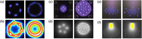
Figure 2. Patterns in plasmas interacting with surfaces. (a) Patterns in a low-pressure cathodic discharge for increasing current (adapted with permission from [31], copyright 2014 IOP Publishing Ltd); (b) patterns in magnetron sputtering for different currents (adapted with permission from [32], copyright 2015 AIP Publishing LLC); (c) patterns in a DBD for increasing driving voltage (adapted with permission from [16], copyright 2015 IEEE); (d) patterns in a cathodic glow discharge for increasing pressure and current (adapted with permission from [18], copyright 2004 IOP Publishing Ltd); (e) patterns on a glow discharge over a liquid anode for increasing current (adapted with permission from [33], copyright 2011 IEEE); and (f) anode patterns in a glow discharge over a water anode for increasing water electrical conductivity (adapted with permission from [34], copyright 2009 AIP Publishing LLC).
Download figure:
Standard image High-resolution imageAt least as rich a variety of patterns are observed in plasmas in contact with liquids, as depicted in figures 2(e) and (f). The patterns in figure 2(e) correspond to an atmospheric-pressure glow discharge in He over a NaCl solution anode for increasing values of current [33], whereas figure 2(d) shows anode patterns in an atmospheric-pressure air glow discharges with a water anode for increasing values of water electrical conductivity [34]. The increasing number of controlling parameters for a liquid electrode (e.g. liquid temperature, electrical and thermal conductivity, pH) and the wider range of intervening phenomena (e.g. vaporization, surface tension and deformation, plasma-aqueous-phase kinetics) makes the study of patterns in plasmas in contact with liquids particularly challenging.
2.2.2. Diversity of patterns.
The richness of patterns observed in electrical discharges is exemplarily depicted by the work of Purwins and collaborators shown in figure 3. Their investigations used a large aspect ratio, parallel plate discharge especially designed to investigate pattern formation and self-organization phenomena. Slight modifications of the experimental setup allow the use of DC or AC applied voltages. The setups (top portions of figures 3(a) and (b)) allow recording the luminescence radiation being emitted from the discharge plane, which is proportional to the density of the electrical current in the gas, and the visualization of patterns through the transparent electrode. Examples of the patterns obtained with the DC setup include (figure 3(a) bottom, clockwise from top-left corner): dynamic chains made of solitary spots, dynamic 'many body' systems made of solitary spots, stationary periodic stripes, and target patterns with zigzag structure, among others [46]. The AC setup patterns encompass (figure 3(b) bottom, clockwise from top-left corner): periodic stripes, dynamic labyrinth patterns, target patterns, and dynamic 'molecule gas' patterns made of solitary spots, among others [47]. The investigators verified that the obtained patterns are not the result of inhomogeneity, which may alter the resulting patterns (often denoted as 'defects' [3]). More information about the setups, the obtained patterns and their analysis can be found in [48, 170].
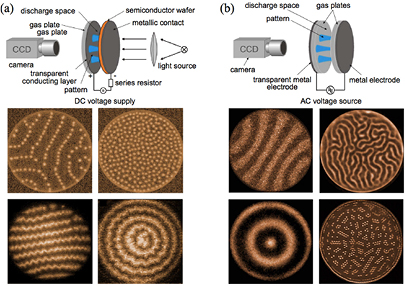
Figure 3. Diversity of patterns in planar electrical discharges. (a) DC discharge, (top) set-up and (bottom) sample patterns (adapted from [46] with permission, copyright 2011 IEEE); (b) AC discharge, (top) set-up and (bottom) sample patterns (adapted from [47] with permission, copyright 2011 IEEE).
Download figure:
Standard image High-resolution imageThe striking diversity of patterns in electrical discharges, as depicted in figures 2 and 3, is unique among other biological, chemical, and physical systems presenting pattern formation. Such diversity, added to the wide range of fluid flow, thermal, chemical and electromagnetic phenomena involved in plasma processes, as well as their nonlinearity, makes the study of pattern formation and self-organization in plasmas particularly challenging.
2.2.3. Role of the intervening surface and medium.
The surface interacting with the plasma constitutes an interface between the plasma and another medium (solid or liquid). The plasma and such intervening medium form, in general, a coupled system in which the surface and the medium fulfill different and complementary roles. For example, the bulk can act as an energy sink for the plasma, whereas the surface can limit fluxes between the plasma and the medium.
The role of the medium is determined by its bulk characteristics, the most important of which are electrical properties. The interaction of plasmas with electrically neutral media is found in plasma surface treatments, the interaction of plasma with substrates [26], as well as in aerothermodynamics, particularly in hypersonic re-entry flows [27, 28]. In such plasma systems, the occurrence of self-organized surface patterns has not been reported. Instead, particularly when bulk fluid motion is predominant, such as in aerothermodynamic flows, the plasma–surface interactions often lead a wide variety of fluid flow, thermal, and chemical instabilities and to turbulence [29, 30], which effectively destroy patterns (see section 3). The interaction of plasmas with electrically active media is more relevant to the study of pattern formation, and is therefore the main focus of this review. The coupled nature of the interaction between plasma and electrically active media is exemplified by the fact that the plasma can alter the medium's bulk properties, a situation often found in plasmas in contact with liquids (see section 5). The plasma-medium coupling can often be neglected from pattern formation analyses by assuming that the medium's properties remain unchanged.
The role of the surface is determined by its topology (e.g. local curvature) and material properties (e.g. chemical bond termination). The use of a nominal planar and uniform surface, such as a flat metal electrode, can often eliminate the role of topology from pattern formation analyses. Nevertheless, such simplification may not be applicable with liquid electrodes, which may present local surface deformation [163]. The role of surface material properties is more complex to investigate, especially when the plasma causes property changes (e.g. re-arrangement of surface bonds, material deposition or evaporation). Moreover, compound material property changes may lead to topological changes, such as variations in surface roughness or the formation of erosion spots. These characteristics are significantly more difficult to analyze than those of the bulk medium, a fact that has limited their systematic investigation within the context of pattern formation.
2.2.4. Current–voltage curve (CVC).
Pattern formation phenomena are often manifested as multiple stable configurations for a single value of a given controlling parameter, such as total current or imposed voltage. Therefore, it is useful to consider how such configurations are manifested within the expected behavior of the plasma, such as within the CVC characteristic of DC electric discharges [49] depicted in figure 4.

Figure 4. CVC for DC electrical discharges. Different types of discharges are distinctively identified by their current range and associated behavior with varying current.
Download figure:
Standard image High-resolution imageThe CVC illustrates the different types of discharges distinctively identified by their behavior with varying current and an associated current range. In a dark discharge, current flows at voltages below the breakdown point, and hence the voltage is not high enough to allow any mechanism to remove electrons from the gas; the discharge relies on background ionization and does not produce appreciable radiative emission in the visible range (and hence its name). The Townsend regime (figure 4, points a to b) is the most relevant type of dark discharge for technological applications. With increasing current, the breakdown voltage is eventually achieved (point b), the discharge becomes self-sustaining, and the plasma achieves the glow discharge regime. The voltage across the electrodes suddenly drops and the current increases to the milliampere range. At lower currents, the voltage varies weakly with current (point c) and the area of the electrodes covered by the glow discharge is proportional to the current; whereas at higher currents the normal glow turns into an abnormal glow (points c to d), the voltage gradually increases, and the discharge covers increasingly more surface area of the electrodes. The electrode coverage can have important implications in the formation of spot patterns (section 4.2).
Glow discharges are produced by ionization by electron impact, which requires that the mean free path of the electrons to be reasonably long but shorter than the distance between the electrodes. Therefore glow discharges typically do not occur at either too low or too high gas pressures. With increasing current the cathode becomes hot enough to directly eject electrons (through thermionic emission) (point d), which then rip off more electrons from the gas causing an avalanche, and the discharge achieves the arc discharge mode. Non-thermal arc discharges are characterized by relatively high electron energy compared to the background gas and decreasing values of voltage across the discharge with increasing current (i.e. a negative slope in the CVC, from point d to e). Thermal arcs occur for higher values of current, and show a positive slope in the CVC (point e onwards). Arcing is a run-away process where the high electrical current causes high heat, which produces even more electrical current until the applied voltage source is depleted of its charge. Such behavior is also of relevance to the formation of electrode spot patterns (sections 4.2 and 4.3).
Even though the main physical characteristics of the above regimes do not change with the occurrence or not of patterns, the specific values of current and voltage do change. This fact is manifested as multiple branches along the CVC, as will be discussed in sections 4 and 5.
2.3. Phenomenology of pattern formation and self-organization
2.3.1. General concepts.
Patterns can be static, dynamic or periodic and oscillatory; they can display discrete spots, also known as solitons, or arrangements of them; they can be formed by continuous structures, which can be regular such as stripes, spirals, targets, and concentric circles, or discontinuous, such as labyrinths; they can be isolated or can tessellate their whole domain. Although spatiotemporal patterns can have any type of dimensionality, pattern formation phenomena are more often found on superficial processes, i.e. processes that occur near an interface or within domains with a relatively large aspect ratio. This is particularly the case for plasma systems, particularly when the plasma interacts with an electrode surface.
Patterns in markedly dissimilar systems are often strikingly similar, which has prompted extensive research efforts for their understanding in terms of general, unifying concepts [3, 50]. The understanding of pattern formation processes is challenging because nonlinear aspects of the system under study largely determine their incidence. The occurrence of pattern formation and self-organization has been associated to the concepts of nonequilibrium, dissipative structures, instability, symmetry breaking, and bifurcation [3, 51].
Pattern formation events frequently couple local processes (e.g. localized heating, reaction fronts, nucleation sites, or electrical connection spots) to global constraints, such as the geometry of the confining domain or a persistent driving force, such as an imposed temperature gradient or electric field. The global behavior involved in pattern formation is often manifested by the dynamic propagation or re-arrangement of local features from a given perturbation (e.g. a dust particle triggering surface nucleation, or nonuniform heating causing the establishment of a convection cell). Sometimes, patterns can display exceptional local features that remain stable; such entities are referred as defects (e.g. analogous to dislocations during crystallization). The (commonly nonlinear) interaction among system components (e.g. bulk fluid motion, temperature gradients, charged species, electromagnetic fields) is essential for the emergence of the self-regulatory characteristics that conduce to the establishment of a pattern. Therefore, pattern formation and self-organization are rightly characterized as manifestations of collective behavior.
2.3.2. Nonequilibrium.
Spontaneous pattern formation phenomena occur in systems outside of equilibrium (i.e. in nonequilibrium systems). A system in equilibrium, in the thermodynamic sense, is isolated and displays no change in its macroscopic properties. Furthermore, local or global perturbations decay and do not alter the overall configuration of the system. The concept of an isolated system has very limited practical application, which has prompted the concept of local thermodynamic equilibrium (LTE), in which equilibrium is achieved locally within the system, but not necessarily through it. (A more thorough discussion of LTE, such as the existence of a Maxwellian velocity distribution in gases, is found in [52].) Most systems of interest show changes in properties due to external interactions (e.g. described as boundary conditions in models of systems with bounded domains) and the assumption of a LTE state is appropriate for their description.
The interaction of a system in LTE with its surroundings at dissimilar conditions maintains the system in a state of (overall) nonequilibrium. Nonequilibrium systems can display macroscopic spatial structure in steady state, which are often referred as dissipative structures [53]. Such structures are favored by the second law of Thermodynamic in the sense that they ensure a high entropy state compared to alternative arrangements of the system. The establishment of such structures is commonly denoted as self-organization. For example, in Rayleigh–Bénard convection nonequilibrium is sustained by the imposed temperature gradient, and the dissipative structures are the convection (recirculation) cells that keep the system in a state of 'structured' equilibrium.
Patterns can also be understood as the result of the competition between production/forcing and dissipation/transport processes. Such competition, exemplified in the discussion of Rayleigh–Bénard convection and chemical oscillations in section 2.1, implies the establishment of fluxes. These fluxes are responsible for the redistribution of a given property (e.g. temperature or concentration) and the interaction of the system with its surrounding (e.g. by the dissipation of heat or mass). The changes in a system in LTE often imply the establishment of fluxes within the system and through the system's boundaries. For example, the recirculation cells in Rayleigh–Bénard convection maintain energy (heat) fluxes between the boundaries and the interior of the domain. The interaction of these competing effects is more clearly observed in reaction–diffusion models, described in section 3.1.
2.3.3. Stability.
The concept of stability, often employed in the study of dynamic systems, is somewhat broader than that of equilibrium. Stability corresponds to the tendency of a system to remain in a given configuration despite the imposition of an external stimulus. Particularly, a system is referred to as unstable if a small perturbation causes it to significantly deviate from its original configuration. Pattern formation and self-organization events are adequately associated to the concept of stability given that a small change in a controlling parameter can trigger the establishment of a spatiotemporal pattern. In fact, stability theory, notably fluid dynamic stability, has been used as one of the main tools for the study of pattern formation, as discussed in section 3.3.
The lack of stability of a nonlinear system is often responsible for bifurcation, chaos, and eventually, turbulence. Bifurcation is the process by which a small change in a controlling parameter leads to markedly different, but well-defined, set of system configurations, such as dissimilar patterns for the same value of the controlling parameter (e.g. different values of voltage for a given value of current in the CVC in figure 4). By continuously varying the controlling parameter, a bifurcation event leads to two or more branches in the characteristic curve of the system, which can be stable or unstable. The intersection of such branches with the line for constant value of the controlling parameter identifies different configurations of the system, which can be recognized as multiple solutions (of a mathematical model) or modes. The stable configurations are the most often found in experiments. Additionally, bifurcation often involves symmetry-breaking. As suggested by its name, symmetry-breaking is the process by which a variation in a controlling parameter produces a configuration with reduced symmetry, e.g. an axisymmetric configuration may evolve into a pattern with a single symmetry plane, or the latter to one with two symmetry planes, etc. Detailed computational studies of bifurcation in plasma systems have been reported in [54] and references therein and in the review article [55] (section 3.4).
Transition to chaos often occurs as a set consecutive bifurcation scenarios. Chaos is referred to (seemingly) random behavior appearing out of deterministic conditions, and is almost exclusively found in nonlinear systems. Chaotic systems display extreme sensitivity to changes in a controlling parameter, which manifests as global deviations in the system dynamics out of relatively small perturbations. Finally, turbulence is regarded as the condition with a continuous state of chaotic changes. A phenomenological progression of the state of a system as function of a controlling parameter is: from a uniform stable configuration to an unstable one; then to the occurrence of bifurcation and the potential formation of patterns (dissipative structures); then to symmetry breaking and the incidence of a wider variety of patterns; and subsequently to chaotic and finally to a turbulent state. It is to be noticed that chaos and turbulence implies the absence of patterns as defined here. Further discussion of the above concepts is found in section 3.3.
3. Modeling and simulation of pattern formation
3.1. Canonical models of pattern formation
The complexity and diversity of pattern formation phenomena prompts the need for simplified, often empirical, models for their investigation. Such models are particularly useful for initial understanding and qualitative analyses. Among approximate, phenomenological or empirical pattern formation models, reaction–diffusion models are perhaps the most widely adopted and effective.
3.1.1. Reaction–diffusion models.
The reaction–diffusion model is one of the simplest and best-known theoretical models employed in the study of pattern formation and self-organization. Reaction–diffusion models haven successfully used to explain self-regulated pattern formation in a diverse variety of systems, such as bacterial and slime-mold colonies, the development of animal embryos [56], the growth of shape or form in plants and animals [8], the evolution of ecosystems [2], chemical oscillation systems [57], excitable systems such as nerve impulse propagation [50]; as well as patterns in electric discharges [58–60].
Reaction–diffusion models are given by a system of equations of the form:
where Y = [yv(t,x)] = [y1 y2 y3 ... yn]⊤ is the vector of n variables with v = {1, 2, ... n} as the variable index and the superscript ⊤ as the transpose operator (i.e. Y is a column vector), t indicates time, x = [xi] is the vector of spatial coordinates with i as a spatial index (e.g. x = [x y z]⊤ for a 3D Cartesian domain),  is the temporal derivative,
  the Laplacian operator (e.g.
  ), D is a diffusion matrix, and the reaction vector S = S(Y) nonlinearly couples the components of Y. The dynamics of a reaction–diffusion system can be understood as the competition between the production, depletion, or forcing of Y given by S and the distribution or transport of Y by the diffusion flux
  . When steady-state
  is reached, the global equilibration between production and diffusion, i.e.
  , can lead to solutions Yss(x) displaying patterns (i.e. the dissipative structures discussed in section 2.3).
The simplest form of a reaction–diffusion model displaying pattern formation is given by a two-component system with Y = [u v]⊤ and no cross-diffusion (i.e. D is diagonal), which is equivalent to:

where u and v are complementary characteristics of the system, Du and Dv are (constant) diffusion coefficients, and Su and Sv the reaction terms, which implicitly couple the two equations.
A distinct example of a model using equations (2) is the activator–inhibitor system, first used by Turing to study morphogenesis [8]. Turing determined that the interaction of two reacting chemicals, an activator that causes an increase in concentration and an inhibitor that causes depletion, can produce a pattern if the inhibitor diffuses faster than the activator (i.e. Du > Dv). In such a system, the functional forms of the reaction terms Su and Sv determine qualitatively the types of patterns obtained, such as discrete (e.g. spots, solitons) or connected (e.g. stripes, spirals) patterns.
3.1.2. Characteristics of reaction–diffusion models.
Even though a large number of pattern formation simulations using reaction–diffusion models use random initial conditions (consistent with the notion of the 'emergence' of patterns), it is to be noticed that the solution to equation (5) is in fact dependent on the initial conditions used. This is depicted in figure 5(a) for the activator–inhibitor model studied in [56] using as initial conditions a random or an analytic (sinusoidal) perturbation of the equilibrium state. In that activator–inhibitor model, the source terms have the form: Su ~ c0 − c1u + c2u2(1 + c3u2)v−1 and Sv ~ d0 − d1u2 − d2v, where ck, dk ⩾ 0 are phenomenological constants. Saturation is established by assigning c3 ≠ 0 (given that the c2 term tends to 0 as u, v  0). As depicted in figure 5(a) (left), when saturation is not included (i.e. c3 = 0), the patterns show periodic cellular structures (solitons) whose spacing retains that in the initial randomly or analytically perturbed field. In contrast, as shown in figure 5(a) (right), when saturation is included, the patterns can develop into labyrinthic sets of semi-connected stripes from a random initial condition, or into a structured set of cellular solitons when a sinusoidal initial condition is used (particularly, spots in between cells can be observed). This dependence on initial conditions can have appreciable consequences in computational and experimental pattern formation investigations.
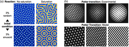
Figure 5. Reaction–diffusion models of pattern formation. (a) Representative solutions with (right) saturation and (left) no-saturation reaction terms and for (top) random and (bottom) analytic initial conditions. The results show the effect of initial conditions on the obtained patterns when a reaction term includes a saturation mechanism. (b) (Top) experimental and (bottom) computational patterns depicting the transition from cellular to strip patterns in a DC planar discharge (adapted from [59] with permission, copyright 1998 The American Physical Society).
Download figure:
Standard image High-resolution imageReaction–diffusion models such as that in equation (2) have also been successfully used to reproduce some aspects of pattern formation phenomena in plasmas. Figure 5(b) shows the transition from hexagonal patterns to stripe patterns by increasing the supply voltage in a DC-driven electrical discharge in nitrogen [59]. The set-up used is similar to the one shown in figure 3(a). The transition from a homogeneous state to hexagon and stripe patterns is relatively well understood theoretically, especially for small-amplitude patterns where the Ginzburg–Landau equation from nonlinear stability theory (section 3.3) is valid [3]. The transition depicted in figure 5(b) occurs with increasing driving voltage, which drives the discharge from the Townsend regime to the glow mode (figure 4). The modeling of the transition shown in figure 5(b) (bottom) used a 2D reaction–diffusion model [61]. Similarly as in the model in figure 5(a), the model in figure 5(b) has a saturation term that prompts to the formation of connected structures. (The model used: Su ~ c0 − c1u − c2uv and Sv ~ d0 − d1v + d2uv + d3uv3(v + d4)−2, where ck, dk ⩾ 0 are model constants.) The development of hexagon clusters consisting of solitary spots occurs via multiplication of the number of spots, which corresponds to the growth of a dissipative structure via a self-completion scenario [59].
Even though reaction–diffusion models can successfully describe important aspects of a plasma system, such as the transition between patterns, their intrinsic semi-empirical nature limits their applicability for further insight or for different types of discharges. Therefore, there is an inherent need to study pattern formation and self-organization using general plasma models.
3.2. Plasma models
3.2.1. Plasma models as transport systems.
Low-temperature plasma processes are rather complicated for their theoretical understanding due to the large diversity of physical–chemical phenomena involved and their nonlinear nature. Such complexity is evident in the mathematical models used to describe them compared to that of other physical, chemical, or biological systems.
Low-temperature plasma models based on the continuum assumption (often denoted as 'fluid models') typically involve a set of conservation equations (e.g. total and/or species mass, linear momentum, energy, etc) derived from moments of Boltzmann equation [62] together with an appropriate set of electromagnetic (Maxwell's) equations, and complemented with material properties and constitutive relations. Conservation equations are expressed in conservative form as  for some conserved variable u = u(t,x) (e.g. mass density ρ, volumetric specific enthalpy ρh, where h is the specific enthalpy), advective and diffusive flux vectors fa = [
 (u)] and fd = [
 (u)], respectively (i is a spatial index), and source term s(u). The set of electromagnetic equations most relevant to low-temperature plasmas (no magnetization, no relativistic, etc) is listed in table 1. In table 1, B denotes the magnetic field, Jq current density, μ0 the permittivity of free space, and Ee the effective electric field (used, in contrast to the real electric field E, to accommodate generalized Ohm's laws consistent with the definition of the constitutive relation for Jq).
Table 1. Electromagnetic field equations.
| Equation | Expression |
|---|---|
| Ampere's law |  |
| Faraday's law |  |
| Generalized Ohm's law |  |
| Gauss's law |  |
| Solenoidal constraint |  |
The set of conservation and electromagnetic equations for a large variety of plasma models can be casted as a single system of transient–advective–diffusive–reactive (TADR) transport equations.
A TADR equation for a generic scalar variable y = y(t,x) is given by:

where  and
and  are the gradient and divergence operators, respectively, A0 is the transient term coefficient, A = [ai] the advection velocity, K = [kij] the diffusivity matrix (i and j are spatial indexes, e.g. i, j = {x, y, z}), and S1 and S0 the first- and zeroth-order reaction terms. Equation (3) is quasi-linear given that the coefficients A0, A, K, S1, and S0 can be functions of y. (Notice that any nonlinearity of the a reactive term can be accommodated by properly defining S1 and S0, i.e. S(y) = S1(y)y + S0(y).) Moreover, equation (3) is expressed in the so-called advective form, which can be obtained from the conservative form by, given u(y), defining:
  ,
,  , and
, and  . The advective form is somewhat more general than the conservative form as the former does not have to be associated to a conserved property or conservation fluxes.
The extension of equation (3) to a system of TADR equations for the vector of unknowns Y = Y(t,x), as needed for denoting plasma flow models, is given by:
where A0, Ai, Kij, and S1 are transport matrices and S0 a vector, which can be function of Y, used to describe each transport process, and Einstein's convention of repeated indexes has been adopted (i.e. summation is implied for any term that contains repeated indexes, e.g.  ). Observe that equation (4) can accommodate different forms of Maxwell's equations, e.g. directly as a first-order system, as a magnetic induction equation in terms of the magnetic field, or as a system in terms of electromagnetic potentials [63].
TADR systems are canonical for the description of transport problems. In fact, TADR systems are often ideal to describe multiphysics and multiscale flow problems, such as incompressible and compressible flows [64, 65], thin-plate elasticity [66], radiation transport [67, 68] problems, and magnetohydrodynamic [69, 70] and nonequilibrium plasma flows [71]. Furthermore, a TADR system is clearly a generalization of the reaction–diffusion system in equation (1), and hence its solution is also prone to the self-organization of patterns.
Of especial relevance for the modeling of low-temperature plasmas are so-called drift–diffusion models and nonequilibrium plasma flow models. Pattern formation studies using such models are presented in section 4. Both types of models are approximations of more general multi-fluid models as described in the review article [72].
3.2.2. Drift–diffusion models.
Drift–diffusion models are particularly suitable for the description of low-pressure discharges and/or when advection (i.e. transport due to bulk fluid motion) is not dominant. These models have been extensively used for the modeling of DBDs (e.g. [17, 72]), 2D and 3D low-pressure–low-current glow discharges (e.g. [45, 73]), and high-pressure glow discharges (e.g. [74]). A drift–diffusion model, as the one used in [45, 75], can be casted as a TADR system by the equations listed in table 2 and using:
where ni and ne denote the number density of ions and electrons, respectively, and ϕ the electric potential. In table 2, Di, De, μi, μe are diffusion coefficients and mobilities for ions and electrons, respectively, α is Townsend's ionization coefficient, β is the coefficient of dissociative recombination,  the electric field strength, ε0 the permittivity of free space, and e the elementary charge. The drift–diffusion model in table 1 has been used for the analysis of bifurcation phenomena leading to the formation in patterns discussed in sections 4.1 and 4.2. More details about these models are found in [45].
Table 2. Drift–diffusion model. For each equation: Transient + Advective − Diffusive − Reactive = 0.
| Equation | Variable | Transient | Advective | Diffusive | Reactive |
|---|---|---|---|---|---|
| Ion conservation | ni |  |
0 |  |
 |
| Electron conservation | ne |  |
0 |  |
 |
| Charge conservation | ϕ | 0 | 0 |  |
 |
3.2.3. Nonequilibrium plasma flow models.
For a general chemical and thermodynamic nonequilibrium plasma flow model, appropriate to describe diverse low-temperature plasmas [76–79], the vector Y can be defined by:
where the vector z specifies the chemical composition of the system (e.g. set of number densities, molar fractions, or mass fractions), p denotes pressure, u mass-averaged velocity, Th and Te heavy-species (i.e. atoms, molecules, ions) and electron temperatures, respectively, ϕe is an effective electric potential, and A is the magnetic vector potential (not to be confused with the advection velocity in equation (3)). Notice that the use of two temperatures but a single bulk velocity makes a model defined by Y in equation (6) a semi-multi-fluid model. Moreover, other variables could be included in equation (6), such a vibrational temperature Tv to describe vibrational energy in molecules or a set of velocities and temperatures for each chemical species as used in multi-fluid models (e.g. [72, 80]).
The increased complexity of including chemical nonequilibrium in a plasma flow model has prompted the use of models relying on the chemical-equilibrium assumption, for which the set of species concentrations are function of the local thermodynamic state only, i.e. z = z(p, Th, Te), and hence do not need to be solver for. Moreover, typically quasi-neutrality is also assumed (i.e.  , where Zs is the charge number of species s (0 for neutral, 1 for first-ionized ions, etc)).
Chemical equilibrium models that further assume LTE in which the energy of all species involved can be characterized by a single equilibrium temperature T (i.e. T = Th = Te) are more commonly used that thermodynamic nonequilibrium (NLTE) models, particularly for the modeling of thermal plasmas (e.g. [81–86]). Nevertheless, thermodynamic nonequilibrium (two-temperature) models have been the only ones so far capable to capture the spontaneous formation of patterns in thermal plasma systems (see section 4.3 and [87, 88]). The chemical equilibrium and thermodynamic nonequilibrium model used in [89–91] is given by the defining Y as:
together with the set of TADR equations in table 3. In table 3, τ is the stress tensor, the sub-scripts h and e are used to denote heavy-species and electron properties, respectively;  is the total derivative, Js is the mass diffusion flux for species s (e.g. Je is the electron mass flux), κ denotes thermal conductivity, σ electrical conductivity, Keh is the energy exchange coefficient [90], εr the net emission coefficient used to describe radiative losses [92], and
  .
.
Table 3. Chemical equilibrium and thermodynamic nonequilibrium plasma flow model. For each equation: Transient + Advective − Diffusive − Reactive = 0.
| Equation | Variable | Transient | Advective | Diffusive | Reactive |
|---|---|---|---|---|---|
| Total mass | p |  |
 |
0 | 0 |
| Momentum | u |  |
 |
 |
 |
| Energy heavy-species | Th |  |
 |
 |
 |
| Energy electrons | Te |  |
 |
 |
 |
| Charge conservation | ϕe | 0 | 0 |  |
0 |
| Magnetic induction | A |  |
 |
 |
0 |
The diffusive term in the equation of conservation of electric charge represents the divergence of the current density Jq, which is given in terms of the effective electric field Ee (table 1). This field is related to the magnetic field B by an electromagnetic potentials formulation, i.e.  and
and  , where ϕe as the effective electric potential and A the magnetic vector potential. The use of ϕp and A allows the a priori satisfaction of the solenoidal constraint
  in Maxwell's equations. As mentioned above, the effective electric field Ee allows the description of generalized Ohm's laws [93]. For example, neglecting Hall effects and charge transport due to ions, the Ee and E are related by:
  , where pe is the electron pressure and ne the number density of electrons. LTE plasma flow models typically assume Ee ≈ E, even though this assumption is not necessary (e.g. for a plasma in chemical equilibrium, the term
  can be calculated as function of the thermodynamic state given by the pressure p and the equilibrium temperature T). The set of transport matrices for the nonequilibrium plasma flow model given by the set of variables in equation (7) and the equations in table 3 is found in [71].
An essential aspect for the formation of patterns is the direct interaction between field variables, more commonly modeled as reaction-like terms (recall Su and Sv in the reaction–diffusion model in section 3.1). The electron–heavy-species energy exchange coefficient Keh in table 3 explicitly couples the two energy equations. Moreover, given its dependence on species mass, collision cross-sections [94, 95], and temperatures Th and Te, this coupling is nonlinear, as often found in pattern formation systems (recall the expressions for Su and Sv terms in the models in figure 5). More details about the NLTE model in table 3 are found in [90, 96].
3.2.4. Comparison of models.
Both drift–diffusion and nonequilibrium flow plasma models are obtained by simplifications of the set of momentum and energy conservation equations for a multi-fluid plasma model [72]. Naturally, both present advantages and limitations which have to be considered before their application to the numerical simulation of a plasma system. A comparison of the models in their treatment of the different phenomena involved in plasma flows is shown in table 4. Generally, drift–diffusion models more suitable for low-pressure systems in which collision frequencies are low, and hence there is weak coupling between the bulk fluid flow and the electromagnetic fields. In contrast, nonequilibrium plasma flow models are more adequate for high-pressure conditions (e.g. from a few Torr to several atm), but are more computationally demanding, which limits the inclusion of detailed chemical kinetics.
Table 4. Comparison between drift–diffusion and chemical equilibrium and thermodynamic nonequilibrium plasma flow models.
| Model | ||
|---|---|---|
| Phenomena | Drift–diffusion | Nonequilibrium plasma flow (NLTE) |
| Mass transport | Assumed negligible, based on background neutral density nn | Mass conservation equation solved to find the pressure field p |
| Species transport | Transport of charged species ni and ne considered, background neutral field nn | Assumed function of thermodynamic state (chemical equilibrium), z(p,Th,Te) |
| Momentum transport | Assumed negligible, based on background neutral density nn | Momentum conservation equation solved to find the velocity field u |
| Heavy-species energy transport | Background heavy-species temperature field Th | Energy conservation equation solved to find heavy-species temperature Th |
| Electron energy transport | Background electron temperature field Te | Energy conservation equation solved to find electron temperature Te |
| Charge transport | Due to transport of charged species ni and ne; charge accumulation possible | Quasi-neutrality assumed, ( ) ) |
| Electromagnetism | Gauss's law considered; magnetic field assumed negligible | Complete set of non-relativistic Maxwell's equations solved (ϕe, A) |
Both plasma models have to be complemented with the calculation of thermodynamic and transport properties, which for are typically highly nonlinear and computationally complex and expensive (e.g. [97–102]), and add further coupling among model variables. Furthermore, it can be noticed that both models, after spatial discretization, lead to differential-algebraic systems of equations due to the presence of zero transient terms (in the charge conservation equation), which leads to the matrix A0 in equation (4) being singular.
3.2.5. Conditions and controlling parameters.
An important aspect of the modeling of plasmas interacting with surfaces is the handling of plasma-surface interactions (section 2.2.3). Such interactions are particularly relevant in low-pressure plasma processing, where surface chemistry can have a dominant role in the overall plasma [72]. The detailed modeling of energy transfer in the cathode region is also particularly relevant for arc discharges [103, 104]. In regard to the modeling of pattern formation in plasmas, more appropriate handling of plasma–surface interactions has been used for drift–diffusion models [45] and the thermal modeling of cathodes [103] than for the nonequilibrium plasma flow models in [87, 88]. At a minimum level of model complexity, plasma–surface interactions are included by the imposition of boundary conditions.
Controlling parameters most often appear in the plasma model through the specification of boundary conditions, e.g. by specifying a given inflow mass rate, pressure, current, driving voltage, or cooling rate. Additionally, controlling parameters can enter the model as material properties, e.g. as a specified value of electrode electrical conductivity. The imposed initial conditions also play a role in time-dependent problems, e.g. when the system is driven to the establishment of dynamic patterns or in conditions such as those depicted in figure 5(a). It is through the variation of controlling parameters that the system is driven to a state that prompts the self-emergence of patterns (e.g. instability, bifurcation), as discussed next.
3.3. Theoretical methods
3.3.1. Plasma models as dynamic systems.
The study of pattern formation and self-organization phenomena is often rooted in the study of dynamic systems. A dynamic system describes the time evolution of the system's variables, typically through a set of nonlinear differential equations for given a set of controlling parameters, i.e.:

where Y = [yv(t,x)] is the state vector (e.g. set of variables in equation (5) or (7)) with v as a variable index, F = [fv(Y;R)] is a vector function (e.g. set of equations in table 2 or 3), and R = [Rp] is the vector of controlling parameters (e.g. quantities used in the specification of constraints, boundary conditions, etc) with p as a parameter index. A semi-colon is used to denote parametric dependency. Equation (8) can be understood as a generalization of the TADR system in equation (4) (i.e.  , assuming A0 is invertible) in which the dependence on controlling parameters is indicated explicitly.
3.3.2. Stability theory.
The first theoretical tool for the study of pattern formation and self-organization is often stability theory [3]. As described in section 2.3, pattern formation occurs in systems outside of equilibrium. Furthermore, the incidence of pattern formation is only possible after the system has passed a state that is a minimum threshold beyond which the system can be considered unstable. Such threshold is given by some critical value of a controlling parameter Rc. Perturbations in the system that reduce the value of the control parameter below Rc decay, whereas those above Rc growth producing a macroscopic change in the system. This behavior of a dynamic system is schematically depicted in figure 6(a). Furthermore, figure 6(b) depicts the steady-state response (output) of a system for increasing R. At R = Rc the system is neutrally stable and presents an initial bifurcation in which a solution may be stable (dominant) whereas the other unstable, and a pattern can occur, e.g. through symmetry-breaking of the solution for lower R. It is the stable solution that often presents patterns (recall that dissipative structures are favored by the second law of thermodynamics). Increasing the value of R leads to subsequent bifurcation events and to multiple solutions, i.e. multiple values yss in f(yss; R) = 0. For even larger values of R the system is driven to a state displaying spatiotemporal chaos, characterized by extreme sensitivity to perturbations, and eventually to turbulence. The progression to chaos and turbulence is not dominantly found in systems that bifurcate because often times other phenomena eventually becoming dominant (e.g. transition from field emission to thermo-field or thermionic emission in DC discharges, depicted in figure 4). A useful summary of bifurcation theory particularly relevant to plasma systems is found in [54].
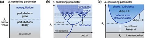
Figure 6. Phenomenology of pattern formation. (a) Patterns form when a controlling parameter (e.g. driving voltage, total current) exceeds a critical value Rc after which small perturbations rapidly grow until a new configuration, displaying a patterned structure, is established. (b) Response of a system as function of a controlling parameter, depicting the occurrence of bifurcation events and the eventual reaching of chaotic and turbulent states. (c) Linear stability theory allows identifying the occurrence of patterns as function of the amplitude of a spatial perturbation (~k−1) and controlling parameter R.
Download figure:
Standard image High-resolution imageStability theory allows obtaining a first approximation of the value of Rc. Given a scalar variable y(t,x) whose dynamics are controlled by a single parameter R and are given by the equation  , stability theory starts by investigating the dynamic behavior of small perturbations
  with respect to a given steady reference state
  , i.e. y(t,x) =
  , where it is implied that
  . The perturbations are assumed to be amenable to a plane wave decomposition, i.e.
where A represents the amplitude of disturbances, i is the imaginary unit, k the wave number vector characterizing the spatial distribution of the perturbation; ω represents frequency and σ = −iω growth rate (not to be confused with electrical conductivity), either of which characterizes the temporal evolution of the perturbation.
After replacing the expansion in equation (9) in the dynamic equation, one obtains a relation between k, R, and σ referred as the dispersion relation, e.g. σ = σ(k;R). Algebraic dispersion relations are obtained for simpler problems (e.g. 1D, weakly-coupled systems) and are amenable to theoretical analyses, whereas differential and nonlinear dispersion relations arising from more complex problems have to be tackled from a computational standpoint (section 3.4). The dispersion relation leads to the identification of regions where the system is expected to be stable or unstable. The instability of the system implies σ > 0, which produces an exponential growth in y'. More generally, given that σ can be a complex number, instability implies Re(σ) > 0; whereas Im(σ) = 0 indicates stationary instability and Im(σ) ≠ 0 oscillatory instability, where Re and Im denote the real and imaginary parts of a complex number, respectively.
Linear stability theory is often adequate for an initial understanding of pattern formation processes because it is relatively straightforward to implement (e.g. using linear decompositions such as equation (9)), depicts the type of dependence of some underlying process parameters (e.g. parameter R), and can be used to determine a characteristic length scale of pattern formation (i.e. ~k−1, where k = ||k|| and || · || denotes the vector norm). Figure 6(c) depicts the type of results obtained with stability theory. Excitations of a given size (k−1) are required for the occurrence of patterns for a given value of R. The threshold of instability is given by the dispersion curve Re(σ) = 0. The minimum value of R producing instability is the critical value Rc for perturbations of size ~ . The region of instability is given by Re(σ) > 0; it is only within this region that patterns can be expected to appear. Nevertheless, these patterns can be stable, static or dynamic, or unstable. For large values of R within the instability domain, the patterns are often effectively destroyed and the system is driven to a state of spatiotemporal chaos and turbulence (section 2.3).
3.3.3. Stability of reaction–diffusion models.
An exemplary example of the use of linear stability theory for the analysis of pattern formation was given by Turing of an activator–inhibitor system, which established what are known as Turing parameters [8, 50]. The system describes the interaction between and activator u and an inhibitor v and is given by the reaction–diffusion model given by equation (2). The analysis starts with the linearization of the reaction terms Su and Sv around reference states (assumed uniform), i.e.  and
and  , where
  and
and  , which leads to:
where Suu, Suv, Svu, and Svv are results of the linearization of Su and Sv (e.g.  ,
,  ), and Dv > Du (i.e. the inhibitor diffuses more rapidly than the activator, see section 3.1). The sign convention used in the linearization in equation (10) is such that, if Suu, Suv, Svu, Svv > 0, then an increase in u causes and increase in both u and v; whereas an increase in v, a decrease in both. The analysis leads to the formation of patterns when [50]:
The controlling parameters are the diffusion coefficients and the functional form of the source terms. These are often chosen empirically in order to reproduce the occurrence of certain types of patterns, and the relations in equation (11) can guide such selection to ensure the occurrence of patterns.
Linear stability theory has also been used for the analysis of diverse plasma systems [105–107]. For example, a linear stability approach was used by Yang and Heberlein to investigate theoretically the instabilities in the anode region of atmospheric pressure arcs [23]; particularly to understand the origin of multiple anode attachments manifested as self-organized erosion patterns (section 4.3).
3.3.4. Nonlinear stability theory.
Despite its advantages, linear stability theory allows for the unphysical prediction of exponentially growing solutions. This limitation, among others, has motivated the development of nonlinear stability theory [108].
In nonlinear stability theory, the decomposition given by equation (9) is extended by allowing A to be a function of time and space, i.e. A = A(t,x). The magnitude of A quantifies the strength of the disturbance. Using the plane wave decomposition in equation (9) considering A(t,x) and after proper scaling, one arrives to an equation for the evolution of the amplitude A of the form:
where ε ~ (R – Rc)/Rc, indicates the deviation from the critical parameter Rc. Equation (12) is known as the Ginzburg–Landau equation and is extensively used in the investigation of spatiotemporal chaos. The equation describes the evolution of the amplitude A due to the competition between growth (+εA term) and saturation (−|A|2A) in the presence of continuous dissipation ( ).
).
Spatiotemporal chaos, which is responsible for the destruction of patterns, manifests itself in all the systems that naturally display pattern formation and self-organization [3], and its incidence is more adequately described by equation (12). Although a powerful tool, the use of nonlinear stability theory has hardly being used in the analysis of low-temperature plasmas, likely due to the complexity and marked nonlinearity of low-temperature plasma models (section 3.2).
3.4. Computational approaches
Computational approaches provide a new dimension, in addition to experimental and theoretical methods, for the investigation of pattern formation and self-organization. These approaches allow the analysis of more comprehensive plasma models than those feasible by theoretical methods, and provide more detailed results and allow more control of parameters and conditions than experimental strategies. Pattern formation in plasma systems can be computationally studied through two main strategies: computational stability/bifurcation analysis and computational experimentation.
3.4.1. Computational stability/bifurcation analysis.
The computational stability/bifurcation analysis approach is a natural extension of the theoretical methods of stability theory in the previous section and depends on the assumptions made on the form of the perturbations. To analyze the stability of a plasma system, similarly as in equation (9), the variable Y (e.g. equation (5) or (7)) is decomposed into a reference solution  (typically static) and a time-dependent perturbation
  , i.e. Y(t,x) =
  (where, as before, it is assumed that
  ) and the decomposition is inserted into equation (4). Different analyses are obtained based on the form of
  , e.g.:

where  is a (constant) vector of amplitudes,
  a space-dependent vector of amplitudes and
  its discrete counterpart,
  is the advective–diffusive–reactive transport operator (see equation (4)), the overbar denotes quantities evaluated at
  , and the matrices M, L, and vector N are obtained from the spatial discretization of the discretized system of partial differential equations (PDEs) (e.g. by a finite differences, finite volume, finite element, or spectral methods). Notice that A0, and hence M (often denoted as the mass matrix), is usually singular due to the charge conservation equation [71]. For both options in equation (13), as before, if Re(σ) > 0, then perturbations (instabilities) tend to grow and the system becomes unstable.
The first option in equation (13) is a dispersion relation of the form σ = σ(k;R), which represents a multi-dimensional dispersion manifold (in contrast to the dispersion curve depicted by Re(σ) = 0 in figure 6(c)). In equation (13), the set of controlling parameters R is assumed implicitly incorporated by appropriate means (e.g. constraints throughout the domain or boundary). This option can only be used to analyze harmonic perturbations with the same wavenumber for all variables.
The second option in equation (13) is a discrete generalized eigenvalue problem, with as many solutions (eigenvalues) as the number of unknowns in the discrete problem (i.e. equal to the number of variables times the number of spatial discretization points). Given that this option does not rely on assumptions about the spatial distribution of  , it allows obtaining multi-dimensional (3D, 2D) static solutions with any degree of symmetry. Notice that the controlling parameters are usually implicitly included within M, L, and N, for example, through the imposition of boundary conditions. A computational bifurcation analysis consists on finding the set of static solutions Yss of F(Yss;Rp) = 0 for a given value of a controlling parameter Rp in R. A detailed description of the mathematical formulation of the theory of multiple solutions and explanation of the different modes for glow and the cathode region of arc discharges is found in the review paper [55].
Computational stability/bifurcation analyses pursued by the first option in equation (13) are the most conservative (and potentially simpler to analyze), whereas those following the second, the most general and hence of greater relevance to plasma systems. Therefore, the rest of the section will mostly address the latter ones. (Other types of stability relations are possible with different assumptions for  ; these usually stand somewhere in between those in equation (13) in terms of comprehensiveness and applicability.)
The computational stability/bifurcation analysis approach has been pursued extensively in fluid dynamics (e.g. [109]) and has been exemplarily demonstrated by the work of Benilov and collaborators for plasma systems (e.g. [54, 55, 110]). The computational complexity and cost of solving the eigenvalue problem in equation (13) for a given value of a controlling parameter Rp is at least comparable to the solution of the actual plasma model. (Notice that the continuous variation of every parameter Rp in R may lead to a response of the system similar to that depicted in figure 6(b).) Therefore, the computational stability/bifurcation analysis approach requires the use of eigenvalue solvers for large-scale problems, such as those obtained from the discretization of PDEs. For example, the eigenvalue solver in Comsol Multiphysics® [111] has been extensively used for this purpose (e.g. [110]). Additionally, these analyses are often complemented with steady-state (static) plasma solvers (which solve: F(Y) = 0) together with continuation strategies to advance the solution in Rp space. Furthermore, in practice, to limit the complexity and computational cost, computational stability/bifurcation analyses often exploit the concept of symmetry breaking by starting from a fundamental mode solution, and then seeking solutions for a deviation of the controlling parameter R (e.g. driving voltage, current) using as initial guess the fundamental solution appropriately perturbed (e.g. by the systematic insertion of noise). For example, given an axi-symmetric solution, a fraction of the domain (wedge) can be used to find a higher mode solution. In fact, the search for higher mode solutions often requires the systematic use of sub-domains with a controlled degree of symmetry [110].
A limitation of the computational stability/bifurcation analysis approach is that it can only be used to find static solutions F(Yss) = 0 (given the assumption of the time-dependency of the growth factor, i.e. exp(σt)). Therefore, dynamic solutions can, in general, not be obtained by this approach. Such solutions can be expected for large values of a parameter Rp, and are depicted in figure 5(b) by the output of the system for large values of R (i.e. after several bifurcation events).
3.4.2. Computational experimentation.
The computational experimentation approach basically consists on performing numerical simulations that allow the potential observation of pattern formation events. Similarly as for physical experiments, this approach will most often lead to the dominant solution. Alternative solutions could potentially be obtained, similarly as for the computational stability/bifurcation approach, by properly inserting controlled perturbations into the fundamental mode solution.
The simulations in computational experimentation have to be based in mathematical models that adequately describe the phenomena driving the formation of patterns. The selection of the adequate mathematical model may not always be evident, particularly when diverse types of coupled phenomena are involved (e.g. electrode material evaporation, electrode heating). For example, drift–diffusion models require a proper set of ionization and recombination mechanisms or a thermal plasma flow model may need to include NLTE to lead to the formation of patterns. Moreover, this approach requires the use of 3D time-dependent models, even for 2D and time-independent (static) configurations of the system geometry and controlling conditions, in order not to restrict potential solutions (e.g. the use of an axi-symmetric model immediately removes the possibility of finding 3D solutions). A limitation of this approach is that a numerical solution may be unstable in the vicinity of the bifurcation point, which may manifest as lack of convergence, but can be stable beyond this vicinity.
The computational experimentation approach can be pursued by basically any appropriate time-dependent plasma solver, such as the general PDE solver in Comsol Multiphysics® [111] for drift–diffusion models; Comsol's Plasma Module for diverse types of low-temperature discharges [112]; or a computational fluid dynamics (CFD) solver appropriately customized for the modeling of plasma flows, such as Ansys Fluent® [113], which has been extensively used for the modeling of diverse thermal plasmas using LTE (e.g. [76, 81, 114]) and NLTE models [89, 91]. The computational experimentation approach has been successfully used in [58] to investigate a DBD using a drift–diffusion model and in [87, 88] to study the spontaneous emergence of patterns in the anode region of an arc discharge using a nonequilibrium plasma flow model (section 4.3).
3.4.3. Numerical and computational challenges.
Both computational approaches need to ensure that the simulations are performed with enough numerical resolution to ensure convergence to discretization-independent solutions. Particularly, for computational experimentation, the discretization of the spatial domain has to ensure enough resolution to resolve the emergence of patterns due to a perturbation of a given wavenumber k (i.e. the local spatial mesh size, e.g. Δx, has to be smaller than the value of k−1). Similarly, the temporal resolution (i.e. the size of time step Δt) has to be small enough to allow the development of transient perturbations in a time scale ~σ−1. The results in section 4.3 demonstrate the sensitivity of the results to the spatial discretization in the case of the simulation of anode patterns in an arc discharge.
Furthermore, the results from computational approaches may depend on the numerical methods used to discretize the TADR system of equations, such as the order of the stencil in finite difference methods, the type and order of elements in finite element methods (FEMs), and the use of upwind strategies, shock-capturing, or total-variation-diminishing approaches, common in CFD and the solution of in advection-dominated transport problems.
A further advantage of computational approaches, not shared by experimental methods, is that they allow a systematic analysis of the effect of different components of the mathematical model. For example, the advective terms in the TADR model can be explicitly suppressed from equation (13) (i.e. by replacing  with
with  as in reaction–diffusion models), which would lead to a different dispersion manifold Re(σ') = 0. The difference between this manifold σ' and the original one σ (from Re(σ) = 0) indicates the role of advective transport to the stability of the system. The results in [54] exemplify this analysis strategy, by showing the marked difference among the CVCs for a glow discharge obtained with a 1D model, with and without diffusion, and the one obtained with a 2D model, which more appropriately captures the expected behavior of the system.
4. Patterns in plasmas over solid surfaces
4.1. Patterns in planar discharges
As described in section 2.3, pattern formation is more often found in superficial processes, such as those over electrodes, and particularly in systems with large aspect ratios (parallel plates, thin slits, etc). In these discharges, cathode and anode phenomena, or more appropriately phenomena along the confining electrodes, are typically highly inter-related. Parallel plate dielectric barrier and cathodic discharges [18] are prominent examples of these types of plasmas and have been extensively used in the investigation of pattern formation and self-organization phenomena.
The studies by Purwins and collaborators using a DC- or AC-driven planar discharge and depicted in figure 3 exemplify the richness of patterns found in these systems. A relatively similar configuration is the DBD system used in [58] and depicted in figure 7. The set-up used is shown in figure 7(a) and was operated in a transient glow discharge regime for different types of gases (He, Ne), pressures, driving voltages, and frequencies. Plasma filaments across the gap are captured as solitons in the observation window, which exhibit particle-like behavior, with motion, generation, annihilation, scattering, and collective interactions leading to the formation of self-organized patterns. The observed patterns, depicted in figure 7(b), included hexagonal solitons, labyrinths, spirals, rings, as well as uniform and hybrid patterns. These types of patterns have also been observed in DBD cryoplasmas [115], of interest for low-damage plasma materials processing.

Figure 7. Patterns in DBDs. (a) Experimental set-up; and (b) a sample of the obtained patterns; from top-left clockwise: hexagonal filamentary solitons, labyrinth structure, hybrid structure, spiral, homogeneous, and concentric ring pattern. Adapted from [58] with permission, copyright 2014 IOP Publishing Ltd.
Download figure:
Standard image High-resolution imageThe authors in [58] observed the possible coexistence of different discharge regimes at different locations within or at different times (e.g. a glow discharge filament can be surrounded by a lower current Townsend discharge region at a slightly different time), which may explain the complexity of the observed patterns and stresses the need for analyses that do not rely the symmetry of patterns.
Dong and collaborators [116] observed a variety of patterns of filaments in a DBD, including spirals, and hexagonal and square lattices, and found a correlation between the temporal dynamics of individual filaments with the change of the spatial symmetry of the patterns as the applied voltage increased, as well as collective vibration of the patterns.
The studies of microdischarges in DBD in air at atmospheric pressure by [19] revealed the formation of patterns reminiscent of 2D crystals. These results correlate with those in [117], in which the quasi-crystal patterns are associated to the self-organization of Voronoi tessellations, which may have potential for applications. The results corroborate the observations of random patterns in [118]. These complex patterns could be associated to modes approaching a state of spatiotemporal chaos (see figure 6).
The suitability of drift–diffusion models for the study of pattern formation and self-organization in DBDs, particularly through computational experimentation, has been fairly well established. For example, the 3D numerical simulations of a DBD discharge using a drift–diffusion model reported in [119] showed quantitative agreement with experimental results (obtained with similar set-up as to the one depicted in figure 3(b)), especially of the filamentary patterns across the gap during the first breakdowns. Moreover, the experimental results in [58] were corroborated and complemented with computational analyses using a 2D drift–diffusion model. The predictive capabilities of the model were contrasted against a reaction–diffusion model (i.e. equation (2) using Su ~ c0 + c1u − c2v − c3u3 and Sv ~ d1u − d2v, where ck, dk ⩾ 0 are model constants), which was properly assessed as an activator–inhibitor system in which the activation is due to ionization in the applied field enhanced by the surface charges, whereas the inhibition is due to the charging of the dielectric which limits the diffusion of filaments and leads to the formation of side filaments beyond the inhibition region. In addition, the work in [17] showed the self-organization of single filaments during a single pulse of a DBD. Their comprehensive 2D model included species transport, electron energy transport, charge accumulation on the surfaces, radiation transport, photo-ionization and encompassed the dielectrics and gas domains in the solution of the charge conservation equation. The authors proposed that the dominant cause for the formation of filamentary patterns is the accumulation of charge on the surfaces of the bounding dielectrics that reinforces successive discharge pulses to occur at the same locations; together with a secondary cause due to the electrostatic repulsion of individual plasma filaments. These mechanisms depict the competition between production/forcing and dissipation/transport processes discussed in section 2.3.
4.2. Cathode patterns
The processes leading to pattern formation and self-organization in plasma electrodes are markedly different between cathodes and anodes. Cathode pattern formation can usually be investigated by partially isolating the cathode region or by neglecting phenomena that do not play major roles near the cathode. In contrast, the analysis of pattern formation over anodes often requires an appropriate description of the anode region together with the adjacent plasma.
Glow and arc discharges are among the plasma systems for which the incidence of cathode patterns has been studied the most. The state-of-the-science in the study of pattern formation in cathodes of glow and arc discharges by computational stability/bifurcation approaches is exemplified by the work of Benilov and collaborators (e.g. [55]).
4.2.1. Cathodic and glow discharges.
Experimentally, Schoenbach and collaborators observed for the first time the self-organization patterns of cathode spots in DC glow microdischarges [18]. Their experimental studies showed the existence of two branches in the CVC, both with positive slope (figure 4). For conventional glow discharges in the milliampere current range, the only discharge mode with a positive slope of the CVC is the abnormal glow mode; and for increasing current after a critical value, the discharge transfers from the abnormal glow into an arc. However, the results in [18] showed that it is possible to stabilize the discharge, even in the glow-to-arc transition range by cooling the cathode. Zhu and Niraula [31] studied pattern formations in a cathodic glow discharge. Their results showed a transition from an arrangement of annular and planetary spots to rings for increasing values of current. In contrast to cathodic microdischarges, which are typically obtained in large aspect-ratio planar configurations, more conventional glow discharges may present a greater variety of intervening phenomena, particularly, 3D effects.
Computationally, Almeida, Benilov, and collaborators have extensively studied cathode patterns in glow discharges using computational stability/bifurcation analyses (e.g. [54, 75]). Their work is exemplified by the results in figure 8. Their analyses were based on a 2D drift–diffusion model (i.e. vector Y in equation (5) and equations in table 2) using the simplified cylindrical model geometry depicted in figure 8(a). The driving parameter R in their model was either the average current density  or the voltage drop U across the discharge (either of which can be used to construct the CVC for the discharge). Figure 8(b) shows the portion of the CVC of relevance for this discharge displaying different branches, each of which corresponds to a particular mode of the discharge and a corresponding cathode pattern. The bifurcation points are denoted by 'a' and 'b' along the curves, and the numerical subscripts indicate the order of their occurrence. The multiple branches in figure 8(b) can be contrasted against the base curve corresponding to the uniform solution (blue curve), and depicted as the normal glow part of the CVC in figure 4. The detailed results obtained by the analyses in [55] are hardly afforded by experimental or theoretical means.
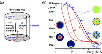
Figure 8. Multiple solutions in glow discharges. (a) Glow discharge model having a cylindrical geometry and voltage drop U or average current density  as controlling parameters. (b) CVC depicting multiple branches and characteristic solution modes, including a single diffuse spot (curve Q) and multiple spot patterns with different degrees of symmetry. Adapted from [54] with permission, Copyright 2008 IOP Publishing Ltd.
Download figure:
Standard image High-resolution imageThe recent work by Bieniek et al [75] demonstrate the suitability of 3D drift–diffusion models using a computational stability/bifurcation analysis together with a stationary solver [111] for the investigation of cathode patterns in glow discharges within a relatively complex geometry, similar to that used in diverse experiments. All the computed spot patterns have been experimentally observed. A review of multiple solutions in DC glow discharges is found in [45] and a detailed description of the theory of multiple solutions in glow discharges is found in [55].
4.2.2. Arc discharges.
In arcs, particularly high intensity discharge (HID) lamps, the formation of cathode spots can severely affect cathode erosion and hence component lifetime [120]. Benilov and collaborators have extensively investigated the existence of multiple solutions in thermionic cathodes in high-pressure arc plasmas (e.g. [103, 104, 121]), manifested by different current transfer spot patterns. Their results stress that the question of stability of steady-state solutions is still open. Their cathode-region model is schematically depicted in figure 9(a). The model was based on the energy conservation equation for the temperature T over the cathode, having as boundary condition the heat transfer to the plasma as function of the voltage drop across the cathode boundary layer U, and as constraint the imposition of a total value of current transferred to the plasma Itot (i.e. Itot =  , where Jq is the current density and Sc the cathode surface). Therefore, model solutions are obtained given the specification of either Itot or U, and hence the steady-state temperature over the cathode is obtained as Tss = Tss(x;U or Itot). Their computational stability/bifurcation analysis approach used a combination of stationary and eigenvalue solvers in Comsol Multiphysics [111]. The obtained results are depicted in figures 9(b) and (c) and elucidate the richness of phenomenological aspects in pattern formation processes over arc discharge cathodes. The results in figure 9(b) correspond to 2D solutions obtained by a zero-gradient boundary condition over the sidewall boundary (i.e. insulated or adiabatic); whereas those in figure 9(c) are 3D solutions obtained by allowing heat conduction through the sidewall. The different curves in figures 9(b) and (c) correspond to different solution modes, and the bifurcation points are indicated with an 'a'. The base curve (in blue) corresponds to the uniform solution depicted as the (non-thermal) arc portion of the CVC in figure 4. These types of analyses can be used to assist cathode design, e.g. by evaluating geometries that favor the stability of a pre-defined mode.

Figure 9. Multiple solutions in cathodic arc discharges. (a) Schematic of the model for the near cathode region; (b) 2D solutions obtained by assuming insulated walls (adapted from [54] with permission, copyright 2009 AIP Publishing LLC); and (c) 3D solutions resulting from considering the sidewall as conductive (adapted from [104] with permission, copyright 2008 IOP Publishing Ltd).
Download figure:
Standard image High-resolution imageThe above arc cathode region model could be extended to include other physical phenomena that may affect the formation of patterns, such the melting and/or evaporation of cathode material, or effects due to bulk fluid flow. For example, the effect of metal evaporation from the cathode on a free-burning arc was studied in [122]. The computational investigations in [122] agreed with experimental observations and revealed that copper evaporated from the cathode causes an increase in electrical conductivity in the anode region, which in turn enhances the constriction of the arc over the anode region. The results revealed higher temperatures in the core and lower temperatures in the arc fringes than when not metal evaporation is included. These results depict the local-to-global coupling in plasma flows, which increases the complexity of the investigation of patterns, particularly over anodes, as discussed next.
4.3. Anode patterns
4.3.1. Anode patterns in arc discharges.
As for cathodes, spot formation over anodes is of relevance to diverse plasma applications, as they can limit process uniformity and electrode life. The formation of anode spots is of particular relevance in HID lamps [123]. The review by Heberlein et al [124] presents a detailed summary of the current understanding of the anode region of electric arcs.
The understanding of pattern formation in high-pressure (atmospheric or higher) arcs is more limited than for other types of plasmas. This is probably due to the harsh conditions typical in these discharges (i.e. high temperatures, current densities, and heat fluxes [52]) combined to the coupled fluid dynamic, thermal, chemical, and electromagnetic phenomena interactions [124]. This limited understanding is evidenced by inconsistent research findings. For example, the experimental investigation in [21] indicate that the transition among multiple anode attachment spots in the free-burning arc occurs due to the development of a thermal instability between Joule heating and gas cooling, whereas the stability analysis and experiments in [22, 23] suggest that multiple anode attachments form only when both, the electron overheating instability and the evaporation–ionization instability, are active. Furthermore, the experimental and theoretical studies in [123] show that the arc attachments on cold (passive) and hot (active) anodes are very different due to the dominance of different types of instabilities.
Computational investigations of anode pattern formation in arc discharges have been scarcer than those of cathode patterns in glow and DBDs (section 4.2). This may be explained by the strong dependence of fluid dynamic effects, such as advective transport (i.e. bulk fluid motion), and strong coupling among fluid dynamic, thermal, and electromagnetic phenomena, which cause large gradients, highly nonlinear interactions and severely increase the complexity of arc discharge models. The larger number of variables, strong nonlinearity and coupling among the equations in the nonequilibrium plasma flow model in table 3 makes computational analyses more expensive and complex than for to the drift–diffusion model in table 2.
Preliminary numerical investigations relevant to the formation of anode patterns in arc discharges is found in [125], which studied the anode region of an arc subject to an impinging flow vertical to the anode surface using a steady-state 2D NLTE plasma flow model. The results captured the experimentally observed diffuse or constricted anode attachments for high and low flow rates, respectively; but lack of numerical convergence was observed for intermediate flow rates, which may be indicative to an underlying bifurcation phenomenon. Computational experimentation with a 3D time-dependent model could lead to the observation of anode spot formation for the intermediate flow rates. Moreover, the study in [126] of a free-burning arc indicates that instabilities inherently develop in a transient and 3D model, which would otherwise be mitigated by the forced symmetry in 2D and/or steady-state models (e.g. the results reported in [81] using a 3D steady-state model did not report the occurrence of anode patterns).
4.3.2. Modeling and simulation of the free-burning arc.
The first report of the spontaneous formation of anode patterns in an arc discharge is found in [87] of a free-burning arc, which has later extended to analyze the effect of anode cooling in [88]. The free-burning arc is a canonical arc discharge extensively studied by theoretical, computational, and experimental means. This discharge is of particular relevance for the study of arc welding (e.g. [127]) and transferred-arc processes (e.g. often found in metallurgy or plasma cutting). Free-burning arc models have been formulated using LTE or NLTE assumptions [128, 129], have considered chemical equilibrium or nonequilibrium [130], have comprised detailed radiative transport [131], and have even included the electrodes within the computational domain [132]. These models have almost exclusively relied on assuming axi-symmetry and steadiness in the solution, which could be expected given the axi-symmetry and steadiness of the geometry and operating conditions. Nevertheless, as described in section 3.4, such assumptions implicitly reduce the number of feasible solutions, and therefore limit the capability of the models to reveal phenomena such as pattern formation and self-organization, which relies on bifurcation and symmetry-breaking.
The investigations of pattern formation in the free-burning arc in [87, 88] used the NLTE plasma flow model given by Y in equation (7) and the set of fluid-electromagnetic equations in table 3. The validation of the NLTE model has been presented in [68, 71, 90, 133] for diverse scalar transport, radiative transport, incompressible, compressible, LTE, and NLTE flow problems.
In the model, heat transfer to the anode qa was modeled as convective heat transfer losses [134] over a water-cooled metal anode driven by the gradient of heavy-species temperature Th, i.e.

where κhr is the translational-reactive heavy-species thermal conductivity,  represents the derivative normal to the anode with n as the unitary vector normal to the anode, hw represents the convective heat transfer coefficient, and Tw = 500 K is used as the reference cooling water temperature. This type of condition is common in CFD and heat transfer, as well as in arc discharge simulations (e.g. [84, 135]). This relatively simple boundary condition allows the simulation of the whole spectrum of cooling levels by varying the value of hw from 0 to
  , i.e.
Equation (15) (top) states that the case of no anode cooling (i.e. zero heat flux from the plasma to the anode) is achieved in the limit  , whereas equation (15) (bottom) indicates that the condition of extreme cooling to a temperature Tw is achieved in the limit
  . Typical values of hw for water cooling range between 200 to 104 W m−2 K−1, and up to 105 W m−2 K−1 if phase change occurs [134, 136]. Other boundary conditions over the anode included zero-gradient for the electron temperature Te, the no-slip velocity condition, and a constant voltage ϕe = 0 V. These conditions can be considered as the simplest for a NLTE model and have been widely adopted by other authors (e.g. [89, 91, 128, 129]).
The computational experimentation approach allowed finding solutions of the form Y = Y(t,x;R), where the set of parameters is R = [hw Itot]⊤ with Itot as the total current over the cathode surface.
The numerical solution of the TADR nonequilibrium plasma flow model given by table 3 was approached using a variational multiscale (VMS) FEM, which has proven been robust and accurate for a wide variety of multiphysics and multiscale problems [137–141], particularly for transport problems related to plasma flows, such as incompressible magnethydrodynamics [142, 143], charge transport in semiconductors [144]. The solution of the resulting time-dependent differential-algebraic system of nonlinear equations was accomplished using a second-order predictor multi-corrector method [145], and the solution of the resulting nonlinear system to be solved at each step with a globalized inexact Newton–Krylov method [146–148]. These methods are closely related to those used in [111].
The study of the free-burning arc in [87] is depicted in figure 10, which shows (a) the model set-up, and (b) and (c), validation results. The domain geometry and conditions are static and axi-symmetric, and did not include the electrode regions. The results in figure 10(b) show agreement with the experimental temperature distributions reported in [128]. The results in figure 10(c) show the expected linear dependence of the voltage drop across the arc |Δϕ| as function of the imposed total current Itot, in agreement with the numerical results in [149] and the experimental findings in [150]. The curve in figure 10(c) is depicted as the (thermal) arc portion of the CVC in figure 4. Furthermore, figure 10(c) shows that the discrepancy in voltage drop with respect to the results obtained with a ~two-times finer mesh are small (the overall difference between the results from the two meshes for other characteristics of the discharge were within 1 and 8% [87]).

Figure 10. Free-burning arc modeling and simulation. (a) Configuration of the system; the domain and imposed conditions are axi-symmetric and time-independent. Depiction of the model validation with: (b) line contours showing (left) the experimental equilibrium (LTE) temperature distribution and (right) computational results of heavy-species temperature (NLTE model); and (c) voltage drop across electrodes as function of current depicting the expected linear variation and the results obtained with a two-times finer spatial discretization. (Adapted from [87] with permission, copyright 2013 IOP Publishing Ltd.)
Download figure:
Standard image High-resolution imageThe computational experimentation followed in [87, 88] did not allowed the observation of multiple branches (or modes) in the CVC (as depicted in the results in figures 8 and 9). Instead, only the dominant solutions were found. This fact is manifested by the single |Δϕ| versus Itot curve in figure 10(c). The simulation results revealed the spontaneous formation of anode spot patterns for varying controlling parameters, as depicted in figure 11. The results in figure 11 show 3D representations of temperature distributions for heavy-species Th (top) and electrons Te (bottom) over the domain for Itot = 200 A. The results for no anode cooling (left), i.e. hw = 0, show a single diffuse attachment over the anode; whereas the results for extreme cooling (right), i.e. hw = ∞, show the emergence of a planetary arrangement of spots in both, Th and Te, distributions.
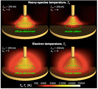
Figure 11. Heavy-species and electron temperature distribution in the free-burning arc. (Top) Heavy-species temperature Th and (bottom) electron temperature Te for (left) no heat transfer to the anode (i.e. adiabatic condition) and (right) extreme cooling of the anode (i.e. fixed anode temperature). The solution for no cooling presents a diffuse plasma–anode attachment, whereas that for extreme cooling displays circular spot patterns observed in both, Th and Te. (Adapted from [88] with permission, copyright 2014 IOP Publishing Ltd).
Download figure:
Standard image High-resolution image4.3.3. Anode pattern formation.
A summary of the solutions of the form Y = Y(t,x;R) with R = [hw Itot]⊤ given by the distribution of heavy-species temperature near the anode surface and depicting the formation of anode patterns is presented in figure 12. The results show the formation of patterned anode attachments with increasing cooling level for a given value to total current Itot. For Itot = 200 A, the anode attachment transitions from axi-symmetric diffuse to patterned with a dominant central spot and a set of smaller, planetary, spots surrounding the main one. This patterned arrangement becomes more accentuated for higher cooling levels. The transition, which can be associated to a bifurcation event given that an axi-symmetric solution should be feasible, occurs for a value of hw ~ 103 and 104 W m−2 K−1. This range for the value of hw is also found in the transitions for Itot = 150 and 100 A. Nevertheless, the obtained patterns for 150 A evolve from planetary and axi-symmetrical to progressively asymmetrical with increasing hw; whereas for 100 A and high cooling levels, the obtained patterns show an asymmetric arrangement of small spots. Asymmetric solutions are particularly puzzling given the axi-symmetry and constancy of conditions.
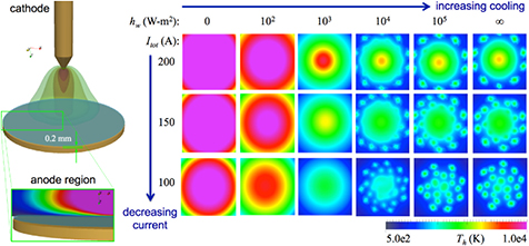
Figure 12. Anode patterns in the free-burning arc. Effect of total current and degree of anode cooling using data from [87, 88]. (Left-top) iso-surfaces of Th depicting the 3D solution; (left-bottom) close-up of the region near the anode; and (right) map of the distribution of Th over the surface 0.2 mm away and parallel to the anode the anode for different values of total current Itot and the convective heat transfer coefficient hw used to model the heat transfer to the anode (i.e. the heat flux from the plasma to the anode is given by: qa = hw(Th − Tw) for a reference value of cooling temperature Tw = 500 K).
Download figure:
Standard image High-resolution imageThe root of this asymmetry is revealed by a set of temporal snapshots of the obtained patterns, which reveal that the patterns for lower currents and higher cooling are in fact dynamic. Such time sequence is depicted in figure 13 for Itot = 100 A and hw = ∞. The results in figure 13 show the formation of new anode spots by the splitting of old ones near the center of the arc, and their subsequent movement radially towards the periphery of the plasma. The observation of dynamic solutions is an advantage of the computational experimentation approach with respect to computational stability/bifurcation. However, the latter allows the identification of multiple solutions. (Computational experimentation may potentially lead to non-dominant solutions for some appropriate type of forcing of the numerical solution or perturbation of boundary conditions.)
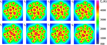
Figure 13. Pattern dynamics in the free-burning arc. Time sequence of the distribution of Th at 0.2 mm above the anode for Itot = 100 A and hw = ∞. The dashed circles emphasize a location where new spots form. (Adapted from [88] with permission, copyright 2014 IOP Publishing Ltd.)
Download figure:
Standard image High-resolution image4.3.4. Sensitivity of numerical solutions.
As discussed in section 3.4, computational pattern formation analyses need to be performed with enough numerical resolution to ensure convergence to discretization-independent solutions. This need is clearly observed by the results shown in figure 14. Figure 14(a) shows experimental anode erosion patterns reported in [23] depicting a central spot and a set of planetary spots, in qualitative agreement with the results described above and presented in figure 14(b) for Itot = 200 A and hw = 104 W m−2 K−1. The results in figure 14(c) correspond to the patterns obtained for the same conditions but using an approximately two-times finer mesh. The comparison of the results in figures 14(b) and (c) clearly indicates lack of convergence to a grid-independent solution. Furthermore, the results in figure 14(c) show certain degree of asymmetry, which, as discussed above, may indicate the onset of a time-dependent solution (e.g. another bifurcation point beyond the transition from a diffuse to a patterned anode attachment).
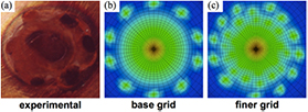
Figure 14. Grid dependency in anode patterns. (a) Experimental erosion patterns over a copper anode; and computational results of Th in the surface 0.2 mm away from the anode obtained with a NLTE model for: (b) a base grid and (c) a two-times finer grid. The results depict the marked dependency of the obtained solutions with the level of resolution of the spatial discretization. (Adapted from [87] with permission, copyright 2013 IOP Publishing Ltd.)
Download figure:
Standard image High-resolution imageIn potential conflict with the need for grid-independent solutions, it has to be considered that the use of progressively finer meshes may lead to spatial discretizations that are incongruent with the physical model used. For example, the assumption of quasi-neutrality in the NLTE model in table 3 implies that variations in the plasma field are larger than the Debye length [49], which clearly imposes a minimum size for the grid spacing. Therefore, a comprehensive computational pattern formation investigation has to concurrently ensure convergence to a grid-independent numerical solution using a physically valid model.
4.3.5. Reduced-order model for anode pattern formation.
The understanding of the mechanisms driving the formation of the above anode patterns is especially challenging due to the complexity of the nonequilibrium plasma flow model used. Reduced-order models, which solve for a sub-set of variables while maintaining the main relevant physical aspects of the system, can be particularly useful for qualitative analyses. Such models can be obtained by suitable approximations of more comprehensive models, such as drift–diffusion and nonequilibrium plasma flow models.
For example, to investigate the role of thermodynamic nonequilibrium, the energy equations in the nonequilibrium plasma flow model in table 3 can be linearized around a reference state (e.g. heavy-species and electron temperatures  and
and  , respectively) in a 2D domain at a distance δw from the anode. Additional approximations lead to a 2D two-temperature reduced-order model of the anode region for the temperature deviations
  and
and  given by:
where the overbars denote properties evaluated at the reference state,  and
and  are (approximate) volumetric heat capacities (notice that hh and he depends on p, Th, and Te),
  is the superficial velocity at a distance δw parallel to the anode (e.g.
  , where
  and
and  are the directional vectors along the x and y axis, respectively),
  is the surface gradient (the z axis is assumed normal to the anode); hw is an effective convective heat transfer coefficient and Tw a reference wall temperature, both used to describe the heat lost to the anode (equation (14)); and
  is a reference value of the electric field.
The system in equation (16) constitutes an advection–diffusion–reaction system, a clear extension of the reaction–diffusion system discussed in section 3.1. The above system describes the competition between energy lost to the anode, energy input through Joule heating, and the equilibration between heavy-species and electron energy and their transport. The formation of anode patterns can be understood as the result of the forcing produced by two competing effects: (i) the loss of energy by heat transfer, which tends to lower the heavy-species temperature Th and (ii) the imposition of a constant value of total current, which tends to maintain high values of electron temperature Te; together with (iii) the equilibration produced by the energy exchange coefficient Keh, and (iv) the overall (advective and diffusive) transport of energy. More effective cooling leads to lowering the value of Th (i.e. for a fixed value of anode heat flux qa and fixed Tw, given qa = hw(Th − Tw), the larger the value of hw, the lower the value of Th), which tends to reduce the electron temperature as well (through the energy exchange term Keh(Te – Th)). But, any decrease in electron temperature Te would cause a decrease in electrical conductivity σ, and hence in current density (given constant  ), which is constrained by the imposition of a total current value (i.e. for a fixed value of total current Itot and anode voltage drop Δϕa, the expression
  , where Jq is the current density and Sa the anode surface, limits the variation in Te through the anode).
The controlling parameters in the model are hw (which controls energy loss) and Itot ~  (which determines energy gain). Therefore, the dynamics of the system could be analyzed by Y = [
 ]⊤, R = [hw Itot]⊤ (similarly as for the NLTE model above), and the expressions in equation (16). The system in equation (16) is in theory amenable to an analysis similar to that by Turing (e.g. equation (11)), except that the strong nonlinearity of the plasma properties make such analysis of little fundamental value, as the reference values can be somewhat arbitrarily chosen.
The reduced-order model in equation (16) seeks to describe the phenomenology of anode pattern formation as a result of competing energy conservation processes. Such explanation is plausibly consistent with the experimental observations and analyses in [21, 22]. For example, the effect of anode material evaporation could be investigated with suitable extensions of the above model and retaining a similar phenomenology: the presence of anode material vapor would increase the electrical conductivity of the plasma, facilitating current transfer, but the phase-change of evaporation is very effective at removing heat from the anode, which would tend to decrease the heavy-species temperature of the plasma.
5. Patterns in plasmas in contact with liquids
5.1. Plasmas in contact with liquids
The study of plasmas in contact with liquids is relevant due to its potential for novel fundamental understanding of the plasma state (e.g. multi-phase plasmas, plasma-driven aqueous kinetics) as well as for their role in established and emerging applications. These applications range from liquid functionalization, water activation and decontamination [35, 36, 151], to nanoparticle and material synthesis [37–41], and to biomaterials processing, bioengineering, and medicine [42, 43, 152–155].
A representative depiction of electrical discharges in contact with liquids is presented in figure 15. Figure 15(a) shows the flow of a non-thermal plasma jet generated from a DBD over liquid water for the inactivation of pathogens, where the liquid surface acts as an electrically-inactive substrate. As discussed in section 2.2.3, the interaction of plasma with neutral surfaces seldom lead to pattern formation; even though the interface is prone to development of diverse types of instabilities. The interaction of a microplasma with a liquid anode is depicted in figure 15(b) for plasma-induced water electrolysis. In this case, despite the electrically-active surface, the formation of surface patterns is impeded by the small size of the plasma–surface interaction region. Specifically, the limited size of the discharge prevents the establishment of the competition between forcing (e.g. plasma kinetics) and dissipation (e.g. species diffusion) processes required for pattern formation. The interaction of a He glow discharge plasma with ambient air over a liquid water anode over a larger interaction area, shown in figure 15(c), does display pattern formation, as described below.
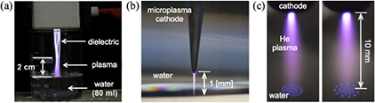
Figure 15. Plasmas in contact with liquids. (a) A non-thermal plasma jet impinging over liquid water for the inactivation of pathogens (adapted from [156] with permission, copyright 2015 AIP Publishing LLC); (b) microplasma over a water anode for plasma-induced water electrolysis (adapted from [157] with permission, copyright 2012 IOP Publishing Ltd); (c) glow discharge over a water anode displaying different types of patterns for increasing current levels (adapted from [33] with permission, copyright 2011 IEEE).
Download figure:
Standard image High-resolution imageThe interaction of plasmas with liquids represents a plasma science frontier involving fundamental issues related to plasma–materials interaction, multi-phase plasma kinetics, and collective effects. The study of plasmas-on-liquids faces distinct challenges due to the broad range, sensitivity, and coupled nature of phenomena involved. For example, whereas deformation and phase-change of the electrode material can often be neglected in the study of discharges with solid electrodes, these phenomena may have a dominant role in discharges on liquid electrodes; or while reactive species rarely interact across and below surface in plasma-materials processing, these species may be transported and react through the bulk liquid (section 2.2.3). Moreover, plasmas-on-liquids present two distinctive types of phenomena: local, across the interface, involving complex plasma and liquid-phase physical and chemical kinetics; and global, along the interface, comprising superficial transport and often the emergence of collective effects such as the self-organization of patterns. Particularly, compared to more conventional electrical discharges, plasmas on liquids show marked sensitivity to pattern formation events and a wider range of intervening parameters.
Electrical discharges in contact with liquids can be distinguished among those within high aspect-ratio configurations (e.g. planar discharges, DBDs) and those within lower aspect-ratios (e.g. jets, columns). The observation of pattern formation in the first type of plasma-on-liquid discharges is exemplified by the work of Dong and collaborators [116, 158] who reported the observation of a rich variety of patterns in a DBD system with two liquid electrodes. The obtained patterns included square-lattices, square-textures, square and hexagonal superlattices, multi-armed spirals, hollow-hexagonals, and rotating-wheels patterns. Despite the inherent increased complexity of having liquid electrodes, these discharges can be expected to display comparable features as those described in sections 2.2 and 4.1. The occurrence of patterns in discharges of the second type is markedly different between those occurring over liquid cathodes and those on liquid anodes.
5.2. Patterns on liquid cathodes
A distinct feature of plasmas with liquid electrodes, compared to solid electrodes, is that the plasma modifies the properties of the liquid. The effect of the plasma on the liquid depends on whether the latter acts as a cathode or anode and if the liquid is dielectric or not.
In a liquid cathode, electrons are transferred to the plasma, whereas plasma ions impact the liquid [159]. The dynamic nature of a liquid cathode is exemplified by the results in figure 16(a) of the acidification and increase in the liquid's conductivity with time by an atmospheric-pressure non-thermal air plasma [44]. The authors in [44] observed that the voltage drop is significantly different between distilled water and electrolyte solutions, whereas acidification of the liquid was always observed. Figure 16(a) also shows the variation in the size of the cathode attachment, temperature, and voltage drop with time. The decrease in the cathode spot size occurs on a larger time scale than that for the drop in pH and hence is correlated with the increase in conductivity. Moreover, the CVC for this discharge showed that for water, the voltage is weakly dependent on current, which is a typical characteristic of mid-current glow discharges; whereas for an electrolyte solution, the voltage variation with current has a negative slope, characteristic of a normal glow discharge (figure 4). Further investigations using advanced spectroscopic diagnostic techniques, as described in the review article [160], revealed the predominance of thermodynamic nonequilibrium in plasma-on-liquid discharges, which is manifested as significant differences in the rotational and excitation temperatures among the intervening species.
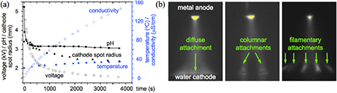
Figure 16. Patterns on liquid cathodes. (a) Variation of cathode spot radius, voltage drop, liquid conductivity, pH, and temperature with time for an atmospheric-pressure non-thermal air discharge over a distilled-water cathode; and (b) characteristic patterns displaying diffuse, columnar, or filamentary attachments over a water cathode observed by different camera shutter times. (Adapted from [44] with permission, copyright 2008 IOP Publishing Ltd.)
Download figure:
Standard image High-resolution imageTypical patterns in plasmas over liquid cathodes are shown in figure 16(b), which show diffuse, columnar, or filamentary attachments over a water cathode observed by different camera shutter times. This dependence on the optical exposure clearly indicates that the formed patterns over the water surface are dynamic. The study reported in [161] using alternate-current excitation observed similar dynamic behavior of the obtained patterns. The macroscopic features across the plasma column (i.e. columnar and filamentary structures) are distinctive characteristics of pattern formation over liquid cathodes, not observed in discharges on liquid anodes.
5.3. Patterns on liquid anodes
In contrast to liquid cathodes, the plasma in contact with a liquid anode supplies gas-phase electrons to the liquid surface, and how these electrons interact with the liquid has not been fully explained [162]. For example, the effect of a liquid electrode on the plasma is also polarity dependent, as represented by the physicochemical mechanism described in [163]. A liquid anode acts as a heat sink for the plasma, which helps stabilize the discharge. This feature is not found in analogous discharges between metal electrodes [164]. Furthermore, temperatures near water anodes have been found to be significantly lower than those for water cathodes [163]. Overall, nonequilibrium is expected in plasmas on water electrodes, even in atmospheric-pressure discharges at low temperatures [164, 165].
As for a liquid cathode, the plasma induces changes on a liquid anode, as shown in figure 17(a) by the change in pH for an atmospheric-pressure AC glow discharge with an electrolyte anode [166]. The results show different rates of decrease in pH with the type of pattern formed: spots, double-rings, or rings; and clearly evidence the relevance of the patterns on the induced physical–chemical kinetics. Figure 17(b) shows the variation of the obtained patterns with pH, depicting the increasingly larger patterns when the liquid changes from acid to neutral. Therefore, the continuous operation of the plasma, which causes the gradual acidification of the liquid, also leads to increasingly constricted anode attachments. Moreover, the results in [166] show that the obtained patterns transitioned from ring-like, to double-ring, and to concentric spots with increasing discharge power.

Figure 17. Patterns on liquid anodes: effect of pH. (a) Variation of electrolyte pH with time for different patterns obtained with an atmospheric-pressure AC glow discharge; and (b) obtained patterns as function of electrolyte pH. (Adapted from [166] with permission; copyright 2015 IOP Publishing Ltd.)
Download figure:
Standard image High-resolution imageIn addition to the effects of the plasma on the liquid, the operating conditions of the discharge produce a diverse range of effects on the obtained patterns, as depicted in figure 18. The effect of total current on the patterns obtained by an atmospheric-pressure DC glow discharge of He on a liquid anode (1% NaCl solution or tap water) is demonstrated in figure 18(a). The obtained patterns transition from a single constricted diffuse spot, to a set of concentric annular patterns, and then to an array of spot patterns for increasing values of current. Figure 18(b) depicts the effect of the imposition of an incident lateral flow of molecular gas on the obtained patterns. The incidence of a stream of N2 over a diffuse uniform (no pattern) anode attachment causes only the deflection of the plasma column. In contrast, the incidence of a stream of O2 causes the emergence of a complex asymmetric spotted pattern at the plasma–liquid interface. Such response is qualitatively maintained for higher flow rates of incident gas. Moreover, further investigations show the emergence of anode patterns due to the diffusion of air on a He discharge, whereas no patterns are observed when a sheath flow of N2 (which limits the entrainment of O2 into the discharge) is used [167].

Figure 18. Patterns on liquid anodes: effect of current and incident gas. (a) The obtained patterns transition from a single constricted diffuse spot, to set of concentric annular patterns, and then to an array of spot patterns for increasing values of current in an atmospheric-pressure DC glow discharge on a liquid water anode; and (b) the imposition of an incident lateral flow of gas causes only the deflection of the plasma column when N2 is used, whereas a complex pattern emerges when O2 is used. (Adapted from [167] with permission, copyright 2014 IOP Publishing Ltd.)
Download figure:
Standard image High-resolution imageThe increased complexity of the experimental investigation of pattern formation and self-organization phenomena in plasmas with liquid electrodes, with respect to that for solid electrodes, is also evidenced in the CVCs shown in figure 19. As for figure 18, a DC glow discharge of He over a liquid anode is used. For both, a 1% NaCl solution or tap water anode, the self-organization of patterns tends to appear for larger inter-electrode spacing and high currents [167, 169]. The emergence of patterns was also found to be dependent on the axial flow rate, with lower flow rates favoring the formation of patterns; as well as on the liquid temperature, particularly on the vapor pressure [167].
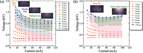
Figure 19. CVCs for glow discharges on liquids. Atmospheric-pressure DC glow discharge of He over: (a) a 1% NaCl solution or (b) tap water anode. A different line is used for a given electrode spacing, whereas a shaded area indicates a specific type of pattern. (Adapted from [167] with permission, copyright 2014 IOP Publishing Ltd.)
Download figure:
Standard image High-resolution imageThe above diversity of phenomena and parameters makes the study of pattern formation and self-organization of plasmas on liquid surfaces more challenging than those over solid electrodes. This fact is particularly evidenced by the lack of theoretical or computational analysis to date. Modeling and simulation of pattern formation of plasmas in contact with liquids could elucidate some of intriguing phenomena driving collective surficial behavior in these discharges.
6. Concluding remarks and outlook
Pattern formation and self-organization are persistent and captivating phenomena commonly observed in both, natural and technological contexts, within diverse varieties of biological, chemical, and physical systems, including plasmas. The study of pattern formation and self-organization phenomena in plasmas interacting with surfaces is important not only for a deeper understanding of nature, but also for their relevance to technological applications that exploit or mitigate self-organization, e.g. from surface activation and texturization, to electrode erosion and process nonuniformity. The diversity of patterns observed in plasmas interacting with surfaces, particularly electrodes, is seldom observed in other types of systems. This diversity, added to the wide range of fluid flow, thermal, chemical and electromagnetic phenomena involved, as well as their marked nonlinearity, makes the study of pattern formation and self-organization in plasmas particularly challenging, which has made their understanding significantly more limited compared to that in other fields, particularly fluid dynamics and biology.
Phenomenologically, pattern formation and self-organization phenomena are related to nonequilibrium, stability, bifurcation and the existence of multiple solutions, and dissipative structures. The study of pattern formation and self-organization in plasmas interacting with surfaces has been based on theoretical, experimental, and computational strategies. Theoretical investigations have been predominantly based on stability theory, dynamic systems, and bifurcation analysis; or on semi-empirical phenomenological models guided by experimental observations and analogies to other system displaying pattern formation (e.g. reaction–diffusion models). Experimental investigations have often relied on specialized configurations designed specifically to explore pattern formation in plasmas. Few reports have indicated the unintended observation of pattern formation events, perhaps due to the sensitivity of these and their often-undesired characteristics. Computational investigations have been distinctly based on stability/bifurcation analyses, which seek to determine the multiple possible static solutions of the system; and on computational experiments, which aim to capture the natural emergence of pattern formation events and to obtain the dominant solution only, which can be either static or dynamic. Both computational approaches are stressed by the need for high numerical accuracy and the use of mathematical models that capture all the relevant processes involved in pattern formation.
Some needs to advance the understanding of pattern formation and self-organization in plasmas interacting with surfaces include:
- Theoretical analyses that explore more comprehensive plasma models, such as multi-fluid and nonequilibrium models with detailed physicochemical kinetics. Such analyses may lead to the determination of characteristic temporal and spatial scales characterizing the patterns, the identification of the values of controlling parameters leading to the onset of pattern formation, and criteria for establishing the occurrence of transitions between patterns.
- Computational analysis methods appropriate to capture the occurrence of pattern formation in general industrial-level plasma solvers. These methods should be based on detailed multi-physics plasma models suitable for the analysis of complex domains with high-accuracy and computational robustness. Furthermore, they should be consistent and complete; this is, they should lead to numerical solutions that are a priori guaranteed to converge to the analytical solution, and should not require calibration parameters. Moreover, these methods should exploit scalable parallel solution strategies suitable for next-generation computational platforms and resources (e.g. [143]).
- Methods capable to track the plasma system beyond the first stages of bifurcation, and which are therefore suitable to capture dynamic solutions and the transition to a spatiotemporal chaos state of the system, and perhaps the eventual establishment of turbulence.
- Computational approaches that lead to solutions independent of the numerical discretization (see section 4.3.4 and figure 20), and that dynamically adapt to the mathematical model most suitable to describe the system (e.g. based on automatic numerical-physical refinement strategies [168]). These approaches would lead to predictive computational tools that can confidently be used for numerical experimentation and scientific discovery.
- Experimental high-resolution non-intrusive spatiotemporal diagnostics, together with analysis strategies that rely as little as possible on assumptions on the system (such as LTE, or Boltzmann distributions).
- Techniques for detailed multi-resolution diagnostics capable to simultaneously track local and global processes, such as species transport across and along the plasma–electrode interface, respectively. These techniques should also be suitable for the analysis of multi-phase systems, particularly for plasmas in contact with liquids.
- Approaches for the control of pattern formation events, either by suppressing or enhancing them. Such approaches could lead to improved applications, such as more resilient plasma–surface treatment processes, and potential to novel ones, such as plasma soliton-based information processing.
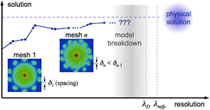
Figure 20. Grid convergence and physical model breakdown. The search of grid-independent solutions by progressive mesh refinement in computational pattern formation simulations faces the challenge of potential model breakdown: the local spacing δ may become smaller than some physical length implied in the continuum model used, such as the Debye length (λD) or mean-free-path (λmfp).
Download figure:
Standard image High-resolution image
The study of pattern formation and self-organization in plasmas interacting with surfaces is an exciting and rich field with many opportunities for greater understanding of nature and potential impact to diverse technological applications.
Acknowledgments
The author acknowledges the financial support provided by the U.S. National Science Foundation through grant PHY-1301935.