

Abstract
We studied the temporal evolution of the electron density distribution in a low pressure pulsed plasma induced by high energy extreme ultraviolet (EUV) photons using microwave cavity resonance spectroscopy (MCRS). In principle, MCRS only provides space averaged information about the electron density. However, we demonstrate here the possibility to obtain spatial information by combining multiple resonant modes. It is shown that EUV-induced plasmas, albeit being a rather exotic plasma, can be explained by known plasma physical laws and processes. Two stages of plasma behaviour are observed: first the electron density distribution contracts, after which it expands. It is shown that the contraction is due to cooling of the electrons. The moment when the density distribution starts to expand is related to the inertia of the ions. After tens of microseconds, the electrons reached the wall of the cavity. The speed of this expansion is dependent on the gas pressure and can be divided into two regimes. It is shown that the acoustic dominated regime the expansion speed is independent of the gas pressure and that in the diffusion dominated regime the expansion depends reciprocal on the gas pressure.
Export citation and abstract BibTeX RIS
Nowadays more and more devices are being connected to the internet. Current predictions indicate that in 2020 more than 25 billion devices will be connected [1]. This results in an increasing global demand for more computational power and memory capacity at higher efficiency. This can be achieved by miniaturizing computer chips. From lithography point of view, for that purpose the next logical step is to use extreme ultra-violet (EUV) radiation at 13.5 nm (92 eV). These high energy photons are partially absorbed by the background gas in the lithography tool, generating a plasma due to photoionization. This EUV-induced plasma is a relatively new phenomenon, which got attention due to the research in the area of EUV lithography [2, 3]. The presence of such plasma can have a long term influence on the optical lifetime of the lithography tool and this influence is yet not fully understood. It is essential to understand the physics of EUV-induced plasmas to predict this impact.
Currently, EUV sources and EUV-induced processes are under huge investigation, for example [4–15]. Recently, Dolgov et al presented an experimental set-up to study EUV-induced processes (e.g. carbon cleaning and ion sputtering) on multilayer mirrors [12]. Moreover, the emission of plasma induced by EUV is studied using optical emission spectroscopy in both man-made plasma [8–11] and astrophysical studies [16, 17]. In previous work, the influence of EUV-induced plasmas on mirrors in the lithography tool was studied using numerical calculations [3, 18]. These authors also attempted to determine the electron density with Langmuir probes, however, they concluded that these probes are not feasible [18]. In recent work we reported the first time-resolved and non-intrusive measurements of the electron density in EUV-induced plasmas in argon by applying microwave cavity resonance spectroscopy [19, 20].
In this contribution we study the expansion of the electron density distribution in EUV-induced plasmas in argon as a function of the gas pressure using MCRS temporally and spatially resolved.
MCRS measurements [21, 22] have been used in other studies to determine the electron density in radio-frequency (RF) plasmas [23–25], discharge tubes [26, 27] and recently in EUV-induced plasmas [19]. Since the method is already extensive described in these publications, we suffice with a brief description of the key concepts only. In MCRS measurements a standing wave is excited in an aluminium (cylindrical) microwave cavity (in our case the cavity as an inner radius of 33 mm and an inner height of 20 mm). The standing waves only exist at specific frequencies, the resonant frequencies  , which depend, amongst others, on the permittivity of the medium inside the cavity. When free electrons are created in the cavity, the permittivity changes, which results in a shift
  of the resonant frequency. The electron density can be calculated from this shift [23]:
where  is the electron mass,
  is the permittivity of vacuum, e the elementary charge and ω and
  are the resonant frequencies with and without plasma, respectively. It should be noted that this method gives the averaged electron density weighted with the square of the local electric field
  of the excited resonant mode [19]:
It should be noted that a single measurement does not contain spatial information about the electron density at all, nor about the expansion of the plasma. Here, we propose the usage of a second mode with a different electric field distribution, meaning that the (spatially dependent) weighting of the electron density is different. Hence, we can obtain spatial information of the electron density, i.e. information about the expansion of the electron density distribution. In our experiments we used two resonant modes, the TM010 and TM110 mode (figure 1). The TM010 mode has a maximum electric field in the centre of the cavity. The TM110 mode has a maximum electric field approximately at half the radius of the cavity (figure 1). This mode has also an azimuthal dependence, however, since the electron density distribution is cylindrically symmetric, the orientation of the mode is irrelevant. In principle any combination of resonant modes can be used, as long as the electric fields of the used modes have a significant different radial dependence.

Figure 1. The electric field in the z-direction of TM010 (left) and TM110 mode (right). This electric field is calculated within the plasimo framework [28, 29].
Download figure:
Standard image High-resolution imageWe obtain spatial information here as follows. Assume we can write the spatial electron density distribution as:

with  the maximum spatial density and f (r, t) a radial distribution function. The electron density measured with the TM010 mode
  is given by:
with  the electric field of the TM010 mode. The electron density measured with the TM110 mode
  is given by:
with  the electric field of the TM110 mode. If we divide
  by
by  , we obtain:
By dividing the weighted densities measured with the TM010 and TM110 mode, we obtain  which contains information about f (r, t). However, f (r, t) still cannot be retrieved directly. This is why we need a set of distribution functions f (r) which describe the general expansion of the plasma. For all these distribution functions we can calculate
  :
:  . Now, we have created a lookup table and can determine f (r) from
  at every moment in time. Hence, we have obtained information about the plasma expansion.
To obtain the set of distribution functions, we used a simplified diffusion model which solves the diffusion equation:
where D is the diffusion coefficient. We are interested in the spatial shape of the distribution only, so the time scale and, hence, the value of D is not important. This is why it is set to 1 here. It should be noted that in the above equation we assume that the electron temperature is always uniform in space, which is an oversimplification. However, it yields a good first approximation of the spatial shapes of the distribution. The cavity is axis-symmetric, so it can be represented with a 2-dimensional (radius r and height z) cylindrical geometry (figure 2). The total computational grid has a radius of 33 mm and a height of 80 mm in order to take into account the plasma outside the cavity. A Neumann boundary condition was applied on the r = 0 axis and Dirichlet boundary conditions on the other boundaries of the grid. On the walls of the cavity we also applied Dirichlet boundary conditions. The initial density distribution is not uniform, but, since the plasma is generated by photoionization, has a similar shape as the EUV beam. Hence, for the initial density distribution (initial condition) in the diffusion model, the shape of the EUV beam is used, which can be approximated by a Gaussian with a full width at half maximum (FWHM) of 2 mm. The diffusion equation is solved using the linear solver in Matlab; the grid has 330 point in the r-direction and has 160 points in the z-direction, the total computational time is a few minutes on a normal desktop computer. At every time step of the simulation, we used the calculated density distribution and the calculated electric fields of the modes to determine the ratio  with equation (6). Furthermore, we averaged the calculated density distribution over the height of the cavity and determined the FWHM of the resulting radial distribution. The calculated ratio
  as a function of the FWHM is plotted in figure 3.

Figure 2. Schematic overview of the geometry used in the diffusion model. The boundary of the grid is spanned by the axis and the dashed lines. A Neumann boundary condition was applied on the r = 0 axis and Dirichlet boundary conditions were applied on the other boundaries of the grid and on the walls of the cavity.
Download figure:
Standard image High-resolution image
Figure 3. The calculated ratio of the electron density measured with the TM010 and TM110 mode versus the FWHM of the density distribution.
Download figure:
Standard image High-resolution imageThe experiment set-up consists of three different chambers (see [20] for detailed information). The source chamber contains the EUV source, which is a xenon-based discharge produced plasma [30]. This source generates an EUV pulse with a duration of 100–200 ns, a repetition rate of 500 Hz and a pulse energy of 44 μJ. A set of elliptical mirrors in the collector chamber focusses the EUV beam in the intermediate focus (IF) located in the measurement chamber. Between the collector and measurement chamber we placed a spectral purity filter (SPF) which only transmits light between 10–20 nm. A cylindrical microwave cavity is placed around the IF. During a measurement we continuously monitor the resonant frequency of the cavity. Details of the diagnostics can be found in our previous publications [19, 20].
We measured the electron density using the TM010 and TM110 modes and determined the ratio  . By comparing the measured ratio with the calculated ratio in figure 3, we obtain the FWHM as a function of time. This FWHM evolution is given in figure 4 for various argon pressures. The results show that the FWHM reaches an asymptote at approximately 17 mm. From our diffusion model we know that this corresponds to a total width of about 63 mm, meaning that the electrons are distributed over the entire cavity, which has a diameter of 66 mm.

Figure 4. The evolution of the FWHM of the radial electron density distribution for various argon pressures.
Download figure:
Standard image High-resolution imageFurthermore, the results in figure 4 show that the plasma expands slower at elevated pressures. We determined the average speed of the expansion by measuring the slope of the FWHM as a function of time between 0.3–1.3 μs. This speed is plotted in figure 5 as a function of pressure. We can distinguish two regimes: a regime at low pressures where the expansion speed is constant and a regime at high pressures where the expansion speed depends reciprocal on the pressure. These two regimes are better visible if we plot the expansion speed times the pressure as a function of the gas pressure (figure 4). At low pressure, the mean free path of the ions is larger than the radius of the plasma. This means that the expansion speed is given by the ion acoustic speed [31]:
with  the Boltzman constant,
  the electron temperature and
  the ion mass. This speed is independent of the pressure and, hence, for pressures for which the mean free path is longer than the radius, we expect a constant speed which is equal to the ion acoustic speed. We call this the acoustic dominated regime. This constant speed is what we observe below 2 Pa. At higher pressures, the mean free path of the ions is smaller than the plasma radius. This means that the expansion speed is determined by the ambipolar diffusion coefficient:
  , with
  mm the typical diffusion length obtained from our diffusion model and
  the ambipolar diffusion coefficient:
where  is the ion mobility at 105 Pa, p is the pressure and
  is the electron temperature in eV [32]. Since
  is inversely proportional to the pressure [32], we expect a reciprocal dependence of the expansion speed on the pressure with a proportionality constant of
  . This reciprocal dependence is exactly what we observe above 3 Pa. We call the regime where the ion mean free path is smaller than the radius of the plasma the diffusion dominated regime.
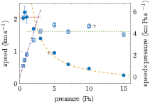
Figure 5. The speed of the expansion of electron density distribution in argon as a function of pressure (•). The fit in the acoustic dominated regime ( ) has a value of
  m s−1and the fit in the diffusion dominated regime (– – –) has a proportionality constant of
  m Pa s−1. For better visibility of the two regimes, we also plotted the expansion speed times, the pressure as a function of the gas pressure (
 ) and the corresponding fits in the acoustic dominated regime (–
  –
– ) and diffusion dominate regime (
 ). The arrows indicate to which axis the graphs correspond. The vertical bars indicate the error.
Download figure:
Standard image High-resolution imageThe transition from the acoustic dominated to the diffusion dominated regime occurs when the mean free path of the ions ( ) is equal to the radius of the plasma (i.e. the ion distribution). The ion neutral collision cross section
  is
is  m2 [32]. We assume that, initially, the radius of the ion distribution is similar to the radius of the EUV beam, which has a total width of 4 mm just after the EUV pulse [19]. This means that the transition occurs at a pressure of about 2 Pa, which is what we observed experimentally (
 Pa).
Pa).
Surprisingly, before the plasma starts to expand, it contracts (figure 6). This could be because the electrons are generated mainly in the centre of the cavity (the location of the EUV beam), i.e. the density in the centre increases faster than near the walls of the cavity. This can lead to a decrease in the FWHM of the electron density distribution, which is observed as a contraction. If this mechanism is causing the contraction, the duration of the contraction is related to the time ionization still occurs. In [20] it was shown that the ionization time is longer at elevated pressures, meaning that also the duration of the contraction should be longer at elevated pressures. Experimentally, however, the opposite is observed, meaning that this mechanism cannot explain the contraction. Another explanation for the contraction is as follows. At the very start of the EUV pulse, electrons which are created run away towards the wall leaving the positive ions behind. This results in a potential difference between the ion core and the wall of the cavity [20]. After this potential difference is established, new electrons created by the EUV beam in the centre of the cavity cannot reach the wall of the cavity due to this potential difference. As a result, these electrons will start to oscillate within the cavity, at certain moments these electrons collide with argon atoms. Due to these collisions, the electrons will lose some of there energy. Hence, the electrons can overcome less potential difference, i.e. the distance the electrons can move away from the ion core becomes smaller as a function of time. As a result, the electron density distribution contracts. The time scale of this contraction is thus related to the collision time of the electrons. This collision time is less than 20 ns above electron energies of 20 eV in 0.5 Pa argon [33], which is much faster than the typical time scale of the contraction. However, due to the cooling of the electrons, the collision time increases to several hundreds of nanoseconds at 1 eV [33], which is comparable to the typical time scale of the contraction.

Figure 6. A zoom in at the start of the evolution of the FWHM of the radial electron density distribution for various argon pressures. The EUV pulse ends at about 120 ns.
Download figure:
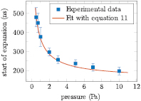
Standard image High-resolution imageAfter the contraction, the plasma starts to expand. The time at which the expansion starts is plotted in figure 7 as a function of the gas pressure. This time is related to the inertia of the ions and, hence, to the inverse of the ion plasma frequency [32]:

with  the ion density and
  the ion mass. In a previous paper [20] we showed that the electron density and, hence, the ion density, depends quadratically on the pressure. This is why the time at which the expansion starts can be fitted with:

where p is the pressure and A, B and C are fitting parameters. The fit in figure 7 is in excellent agreement with the experimental data.
Figure 7. The time at which the electron density distribution starts to expand as a function of the gas pressure. The data is fitted with equation (11).
Download figure:
Standard image High-resolution image
In conclusion, we determined the expansion of the electron density distribution in EUV-induced plasmas in argon using MCRS. It has been shown that EUV-induced plasma, although being a rather uncommon plasma, can be perfectly explained by known plasma physical laws and processes. Due to the cooling of electrons, the electron density distribution first contracts. At the moment the ions start to move, the plasma starts to expand. The speed of this expansion depends on the gas pressure and can be divided into two regimes. In the acoustic dominated regime the expansion speed does not depend on the gas pressure and in the diffusion dominated regime the plasma depends reciprocal on the gas pressure. All subsequent phenomena observed could be perfectly fitted by simplified models.
Acknowledgments
The authors would like to thank ASML for their financial support and the opportunity to use its EUV sources and J van Dijk and D Mihailova for their help with plasimo