


ABSTRACT
We report on a high angular resolution survey of circumstellar disks around 24 northern sky Be stars. The K-band continuum survey was made using the CHARA Array long baseline interferometer (baselines of 30–331 m). The interferometric visibilities were corrected for the flux contribution of stellar companions in those cases where the Be star is a member of a known binary or multiple system. For those targets with good (u, v) coverage, we used a four-parameter Gaussian elliptical disk model to fit the visibilities and to determine the axial ratio, position angle, K-band photospheric flux contribution, and angular diameter of the disk's major axis. For the other targets with relatively limited (u, v) coverage, we constrained the axial ratio, inclination angle, and/or disk position angle where necessary in order to resolve the degeneracy between possible model solutions. We also made fits of the ultraviolet and infrared spectral energy distributions (SEDs) to estimate the stellar angular diameter and infrared flux excess of each target. The mean ratio of the disk diameter (measured in K-band emission) to stellar diameter (from SED modeling) is 4.4 among the 14 cases where we reliably resolved the disk emission, a value which is generally lower than the disk size ratio measured in the higher opacity Hα emission line. We estimated the equatorial rotational velocity from the projected rotational velocity and disk inclination for 12 stars, and most of these stars rotate close to or at the critical rotational velocity.
Export citation and abstract BibTeX RIS
1. INTRODUCTION
Classical Be stars are non-supergiant, B-type stars that are surrounded by hot gaseous disks. This circumstellar gas is responsible for many observational characteristics such as hydrogen Balmer emission lines, IR flux excess, and short- and long-term flux variability (Porter & Rivinius 2003). Optical and infrared interferometry has become an important tool in characterizing Be stars and their disks (Stee 2011). The first interferometric survey of Be stars was made by Quirrenbach et al. (1997) to resolve the Hα emission in seven Be stars. Their survey showed that the emitting regions are flattened, which is strong observational evidence of a disk-like geometry. Quirrenbach et al. (1997) combined optical interferometry and spectropolarimetry to derive the disk position angle on the sky, and they found good agreement between these techniques. Tycner et al. (2004, 2005, 2006, 2008) used the Navy Precision Optical Interferometer (NPOI) to observe the Hα emission from the disks of seven Be stars. Their observations showed that a direct correlation exists between the disk sizes and the net Hα luminosities.
Infrared observations have begun to reveal the spatial properties of the continuum and line emission of Be star disks. Gies et al. (2007) made the first CHARA Array long-baseline interferometric observations in the K-band of four bright Be stars, γ Cas, ϕ Per, ζ Tau, and κ Dra, and they were able to resolve the disks and to constrain their geometrical and physical properties. Meilland et al. (2007) studied the geometry and kinematics of the Be star κ CMa in the Brγ emission line and in the nearby continuum using the VLTI/AMBER instrument. Meilland et al. (2011) observed the Be binary system δ Sco using spectrally resolved interferometry with the VLTI/AMBER and CHARA/VEGA instruments. Their observations show that the disk varies in size from 4.8 mas in Hα, to 2.9 mas in Brγ, and to 2.4 mas in the K-band continuum. Meilland et al. (2012) completed a survey of eight Be stars with VLTI/AMBER and measured the disk extensions in the Brγ line and the nearby continuum. Their study suggests that the disk kinematics are dominated by Keplerian rotation and that the central stars have a mean ratio of angular rotational to critical velocity of Ωrot/Ωcrit = 0.95. In addition, Meilland et al. (2009) used the VLTI/MIDI instrument to determine the N-band (10 μm) disk angular size for seven Be stars.
Interferometry offers us the means to explore Be star disks in large numbers and to begin to understand their properties as a whole. Here we present results from such a survey that we conducted in the K-band continuum using the CHARA Array long-baseline interferometer. In Section 2, we list our sample stars, present our observational data sets, and describe the data reduction process. In Section 3, we describe a method that we implemented to correct the interferometric measurements for the flux of stellar companions. We discuss in Section 4 the spectral energy distributions (SEDs) and their use in estimating the stellar angular diameter and infrared excesses of Be stars. In Section 5, we present fits of the interferometric visibilities using simple geometrical models, and in Section 6, we discuss the results with a particular comparison of the K-band and Hα disk sizes. Finally, we summarize our results and draw our conclusions in Section 7.
2. OBSERVATIONS AND REDUCTION
We selected 24 Be stars as targets for this interferometric survey. The main selection criteria were that the stars are nearby and bright, well within the limiting magnitude of the CHARA Classic tip-tilt servo system (V < 11) and the near-IR fringe detector (K < 8.5). The selected Be stars had to have declinations north of about −15° to be accessible with the interferometer at low air-mass values. Furthermore, most of the targets have recently shown hydrogen emission and a near-IR flux excess. We relied particularly on spectrophotometric and Hα observations conducted by Tycner et al. (2006), Grundstrom (2007), Gies et al. (2007), and Touhami et al. (2010). The targets and their adopted stellar parameters are presented in Table 1. Columns 1 and 2 list the star names, Columns 3–5 list the spectral classification from the compilation by Yudin (2001) and the stellar effective temperature Teff and gravity log g from Frémat et al. (2005, see their Table 9 "Apparent parameters"). The stars HD 166014 and HD 202904 are not listed by Frémat et al. (2005), so we used the parameters for these two from Grundstrom (2007). Columns 6 and 7 list predictions for the position angle (P.A.) of the projected major axis of the disk that should be 90° different from the intrinsic polarization angle (McDavid 1999; Yudin 2001) and for r, the ratio of the minor to major axis sizes according to the estimated stellar inclination from Frémat et al. (2005).
Table 1. Adopted Stellar Parameters
| HD | Star | Spectral | Teff | log g | P.A. | r |
|---|---|---|---|---|---|---|
| Number | Name | Class. | (K) | (cm s−2) | (°) | |
| HD 004180 | o Cas | B2 Ve | 14438 | 3.284 | 164 | 0.582 |
| HD 005394 | γ Cas | B0 IVe | 26431 | 3.800 | 20 | 0.764 |
| HD 010516 | ϕ Per | B0.5 IVe | 25556 | 3.899 | 117 | 0.322 |
| HD 022192 | ψ Per | B4.5 Ve | 15767 | 3.465 | 125 | 0.280 |
| HD 023630 | η Tau | B5 IIIe | 12258 | 3.047 | 124 | 0.727 |
| HD 023862 | 28 Tau | B8 Vpe | 12106 | 3.937 | 159 | 0.438 |
| HD 025940 | 48 Per | B4 Ve | 16158 | 3.572 | 55 | 0.798 |
| HD 037202 | ζ Tau | B1 IVe | 19310 | 3.732 | 122 | 0.071 |
| HD 058715 | β CMi | B8 Ve | 11772 | 3.811 | 140 | 0.779 |
| HD 109387 | κ Dra | B6 IIIpe | 13982 | 3.479 | 102 | 0.660 |
| HD 138749 | θ CrB | B6Vnne | 14457 | 3.745 | 177 | 0.200 |
| HD 142926 | 4 Her | B9 pe | 12076 | 3.917 | 70 | 0.300 |
| HD 142983 | 48 Lib | B3 IVe | 15000 | 3.500 | 50 | 0.405 |
| HD 148184 | χ Oph | B1.5 Vpe | 28783 | 3.913 | 20 | 0.947 |
| HD 164284 | 66 Oph | B2 IV | 21609 | 3.943 | 18 | 0.685 |
| HD 166014 | o Her | B9.5 III | 9800 | 3.500 | 89 | 0.868 |
| HD 198183 | λ Cyg | B5 Ve | 13925 | 3.167 | 30 | 0.826 |
| HD 200120 | 59 Cyg | B1.5 Ve | 21750 | 3.784 | 95 | 0.310 |
| HD 202904 |  Cyg Cyg |
B2.5 Vne | 19100 | 3.900 | 27 | 0.887 |
| HD 203467 | 6 Cep | B2.5 Ve | 17087 | 3.377 | 76 | 0.799 |
| HD 209409 | o Aqr | B7 IVe | 12942 | 3.701 | 96 | 0.364 |
| HD 212076 | 31 Peg | B1.5 Vne | 12942 | 3.701 | 148 | 0.955 |
| HD 217675 | o And | B6 IIIpe | 14052 | 3.229 | 25 | 0.022 |
| HD 217891 | β Psc | B5 Ve | 14359 | 3.672 | 38 | 0.943 |
Download table as: ASCIITypeset image
Measuring the instrumental transfer function of the CHARA Array interferometer is performed by observing calibrator stars with known angular sizes before and after each target observation. The calibrator stars are selected to be close to the targets in the sky, unresolved with the interferometer's largest baseline, and without known spectroscopic or visual binary companions. We collected photometric data on each calibrator star in order to construct their SED and to determine their angular diameter. The collected UBVRIJHK photometry (available from Touhami 2012) is transformed into calibrated flux measurements using procedures described by Colina et al. (1996) and Cohen et al. (2003). The stellar effective temperature Teff and the gravity log g (generally from the compilation of Soubiran et al. 2010) are used to produce a model flux distribution that is based on Kurucz stellar atmosphere models. Note that we generally used Johnson U magnitudes compiled by Karataş & Schuster (2006) and B, V magnitudes from Ammons et al. (2006), who list Tycho B and V magnitudes that are slightly different from Johnson B, V magnitudes. The photographic R and I magnitudes were collected from Monet et al. (2003), which are only slightly different from Johnson R, I magnitudes. The near-IR J, H, K photometry was collected from the Two Micron All Sky Survey (2MASS; Skrutskie et al. 2006). The use of non-standard photometry introduces errors in the best-fit, limb-darkened angular diameter of the calibrators that are comparable to or smaller than the estimated uncertainties given in Table 2. We also collected measurements of E(B − V) and applied a reddening correction to the model SED before fitting the SED of the calibrators. We then computed a limb-darkened angular diameter θLD by direct comparison of the observed and model flux distributions. Based upon the limb-darkening coefficients given by Claret (2000), we transformed the limb-darkened angular diameter to an equivalent uniform-disk angular diameter θUD assuming a projected baseline of 300 m.
Table 2. Calibrator Star Angular Diameters
| Calibrator | Object | Teff | Ref. | log g | Ref. | Spectral | E(B − V) | Ref. | θLD | θUD |
|---|---|---|---|---|---|---|---|---|---|---|
| HD Number | HD Number | (K) | (cm s−2) | Class. | (mag) | (mas) | (mas) | |||
| (1) | (2) | (3) | (4) | (5) | (6) | (7) | (8) | (9) | (10) | (11) |
| HD 004222 | HD 004180 | 8970 | 1 | 4.20 | 2 | A2 V | 0.009 | 3 | 0.303 ± 0.017 | 0.301 ± 0.021 |
| HD 006210 | HD 005394 | 6065 | 4 | 3.86 | 4 | F6 V | 0.009 | 5 | 0.516 ± 0.025 | 0.506 ± 0.035 |
| HD 011151 | HD 010516 | 6405 | 6 | 4.00 | 6 | F5 V | 0.003 | 7 | 0.424 ± 0.011 | 0.416 ± 0.029 |
| HD 020675 | HD 022192 | 6577 | 6 | 4.28 | 6 | F6 V | 0.006 | 7 | 0.418 ± 0.018 | 0.417 ± 0.028 |
| HD 024167 | HD 023630 | 8200 | 1 | 4.01 | 8 | A5 V | 0.016 | 8 | 0.246 ± 0.015 | 0.243 ± 0.017 |
| HD 024357 | HD 023862 | 6890 | 1 | 4.30 | 2 | F4 V | 0.008 | 8 | 0.374 ± 0.014 | 0.368 ± 0.026 |
| HD 025948 | HD 025940 | 6440 | 1 | 4.07 | 8 | F5 V | 0.008 | 7 | 0.374 ± 0.014 | 0.367 ± 0.025 |
| HD 037147 | HD 037202 | 7200 | 1 | 4.13 | 8 | F0 V | 0.003 | 8 | 0.403 ± 0.021 | 0.397 ± 0.028 |
| HD 057006 | HD 058715 | 6166 | 9 | 3.77 | 9 | F8 V | 0.001 | 7 | 0.501 ± 0.031 | 0.491 ± 0.034 |
| HD 111456 | HD 109387 | 6313 | 10 | 4.70 | 10 | F6 V | 0.000 | 7 | 0.477 ± 0.028 | 0.467 ± 0.033 |
| HD 142640 | HD 142983 | 6481 | 4 | 4.09 | 4 | F6 V | 0.005 | 7 | 0.363 ± 0.013 | 0.356 ± 0.025 |
| HD 144585 | HD 148184 | 5831 | 11 | 4.03 | 11 | G5 V | 0.005 | 7 | 0.438 ± 0.012 | 0.429 ± 0.030 |
| HD 159139 | HD 166014 | 9550 | 2 | 4.17 | 2 | A1 V | 0.023 | 8 | 0.248 ± 0.013 | 0.246 ± 0.017 |
| HD 161941 | HD 164284 | 10512 | 12 | 3.67 | 12 | B9.5 V | 0.180 | 3 | 0.194 ± 0.037 | 0.194 ± 0.014 |
| HD 166233 | HD 164284 | 6661 | 12 | 3.57 | 12 | F2 V | 0.003 | 7 | 0.405 ± 0.026 | 0.398 ± 0.027 |
| HD 168914 | HD 166014 | 7600 | 2 | 4.20 | 2 | A7 V | 0.000 | 13 | 0.456 ± 0.023 | 0.450 ± 0.031 |
| HD 192455 | HD 203467 | 6251 | 4 | 4.05 | 4 | F5 V | 0.003 | 7 | 0.504 ± 0.026 | 0.494 ± 0.035 |
| HD 196629 | HD 198183 | 6996 | 14 | 4.25 | 15 | F0 V | 0.007 | 8 | 0.285 ± 0.010 | 0.280 ± 0.020 |
| HD 203454 | HD 202904 | 6146 | 16 | 4.50 | 16 | F8 V | 0.001 | 8 | 0.406 ± 0.025 | 0.398 ± 0.028 |
| HD 211575 | HD 209409 | 6300 | 17 | 4.00 | 17 | F3 V | 0.006 | 7 | 0.367 ± 0.024 | 0.360 ± 0.025 |
| HD 213617 | HD 212076 | 7259 | 18 | 4.40 | 18 | F1 V | 0.017 | 8 | 0.278 ± 0.010 | 0.274 ± 0.019 |
| HD 217877 | HD 217891 | 5953 | 6 | 4.29 | 6 | F8 V | 0.003 | 7 | 0.365 ± 0.149 | 0.358 ± 0.025 |
| HD 217926 | HD 217891 | 6528 | 14 | 3.63 | 8 | F2 V | 0.005 | 7 | 0.335 ± 0.013 | 0.329 ± 0.023 |
| HD 218470 | HD 217675 | 6407 | 19 | 4.07 | 19 | F5 V | 0.004 | 7 | 0.491 ± 0.028 | 0.482 ± 0.033 |
References. (1) Wright et al. 2003; (2) Lafrasse et al. 2010; (3) from B−V and spectral classification; (4) Balachandran 1990; (5) Karataş & Schuster 2006; (6) Valenti & Fischer 2005; (7) Ammons et al. 2006; (8) Philip & Egret 1980; (9) da Silva et al. 2011; (10) Schröder et al. 2009; (11) Edvardsson et al. 1993; (12) Prugniel & Soubiran 2001; (13) Gray et al. 2001; (14) Masana et al. 2006; (15) Allende Prieto & Lambert 1999; (16) Boesgaard & Friel 1990; (17) Boesgaard & Tripicco 1986; (18) Gerbaldi et al. 2007; (19) Fuhrmann 1998.
Download table as: ASCIITypeset image
Columns 1 and 2 of Table 2 list the calibrator star and its corresponding target, respectively, Columns 3 and 4 list the calibrator effective temperature Teff and reference source, Columns 5 and 6 give the surface gravity log g and reference source, Column 7 gives the spectral classification, and Columns 8 and 9 list the adopted interstellar reddening E(B − V) and the reference source, respectively. Column 10 of Table 2 lists the best-fit limb-darkened angular diameter θLD derived from fitting the calibrator SED, and Column 11 lists the corresponding uniform-disk angular diameter θUD.
The observations were conducted between 2007 October and 2010 November using the CHARA Classic beam combiner operating in the K-band (effective wavelength = 2.1329 μm; ten Brummelaar et al. 2005). We need a minimum of two interferometer baselines at substantially different projected angles on the sky to map the circumstellar disks around our targets, and we generally used the southwest baseline of length ∼278 m oriented at 39° west of north (S1/W1) and the southeast baseline of length ∼330 m oriented at 22° east of north (S1/E1). Each target and its calibrator were observed throughout a given night in a series of 200 scans recorded with a near-IR detector on a single pixel at a frequency that ranged between 500–750 Hz, depending on the seeing conditions of each particular night of observation. The interferometric raw visibilities were then estimated by performing an integration of the fringe power spectrum. We used the CHARA Data Reduction Software (ReduceIR; ten Brummelaar et al. 2005) to extract and calibrate the target and the calibrator interferometric visibilities. Then the raw visibilities were calibrated by comparing them to the time-interpolated calibrator visibilities and rescaling them according to the predicted calibrator visibility for the given projected baseline and stellar angular diameter. The resulting calibrated visibilities are listed in Table 3. Column 1 of Table 3 lists target HD number, Column 2 lists the heliocentric Julian date of mid-observation, Column 3 lists the telescope pair used in each observation, Columns 4 and 5 list the u and v frequencies, respectively, Column 6 lists the projected baseline, Column 7 lists the effective baseline (see Section 5.2), Columns 8 and 9 list the calibrated visibility and its corresponding uncertainty, respectively, and lastly, Columns 10 and 11 list the visibility measurements and uncertainties corrected for the flux of stellar companions for those cases with known binary parameters. We will discuss this correction in detail in the next section.
Table 3. Calibrated Visibilities
| HD | Date | Telescope | u | v | Baseline | Effective | V | δV | Vc | δVc |
|---|---|---|---|---|---|---|---|---|---|---|
| Number | (HJD−2,400,000) | Pair | (cycles arcsec−1) | (cycles arcsec−1) | (m) | Baseline (m) | ||||
| (1) | (2) | (3) | (4) | (5) | (6) | (7) | (8) | (9) | (10) | (11) |
| HD 004180 | 54756.622 | S1/W1 | −75.187 | −627.643 | 278.114 | 162.970 | 0.705 | 0.042 | 0.689 | 0.046 |
| HD 004180 | 54756.629 | S1/W1 | −44.906 | −630.398 | 278.055 | 164.379 | 0.693 | 0.042 | 0.838 | 0.045 |
| HD 004180 | 54756.637 | S1/W1 | −15.062 | −631.747 | 278.024 | 166.438 | 0.821 | 0.047 | 0.826 | 0.051 |
| HD 004180 | 54756.649 | S1/W1 | 19.818 | −631.622 | 278.027 | 169.637 | 0.736 | 0.044 | 0.865 | 0.048 |
| HD 004180 | 54756.661 | S1/W1 | 52.167 | −629.866 | 278.067 | 173.303 | 0.767 | 0.048 | 0.793 | 0.053 |
| HD 004180 | 54757.610 | S1/W1 | −91.896 | −625.513 | 278.157 | 162.450 | 0.812 | 0.045 | 0.863 | 0.049 |
| HD 004180 | 54757.626 | S1/W1 | −53.847 | −629.731 | 278.070 | 163.890 | 0.569 | 0.032 | 0.670 | 0.035 |
| HD 004180 | 54757.633 | S1/W1 | −21.944 | −631.555 | 278.029 | 165.906 | 0.724 | 0.041 | 0.762 | 0.045 |
| HD 004180 | 54757.645 | S1/W1 | 11.396 | −631.820 | 278.023 | 168.790 | 0.609 | 0.032 | 0.680 | 0.035 |
| HD 004180 | 54757.657 | S1/W1 | 44.336 | −630.437 | 278.054 | 172.357 | 0.790 | 0.035 | 0.863 | 0.038 |
Only a portion of this table is shown here to demonstrate its form and content. A machine-readable version of the full table is available.
Download table as: DataTypeset image
The internal uncertainties from fitting individual fringes are generally smaller than <5%. The scatter in the data depends mostly on the target magnitude and seeing conditions at the time of the observations, which usually varies with a Fried parameter in the range r0 ≃ 2.5–14 cm. The visibility uncertainties for the brightest targets range between 2% and 5%, while those for the faintest ones reach up to 8%.
Overall we obtained a relatively good set of observations at different hour angles for each star in our sample, with the exceptions of HD 58715 and HD 148184 where the position angle coverage was limited to only one projected baseline. Figure 1 shows the distribution of the observations in the (u, v) plane for our sample.
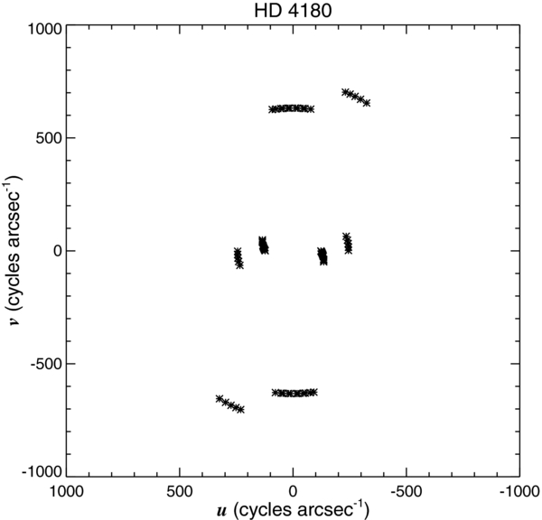
Figure 1.
Sampling of the frequency (u, v) plane for our Be star sample. Observations conducted in this survey are indicated by star symbols while archived measurements from Gies et al. (2007) are shown by diamonds. (The complete figure set (24 images) is available in the online journal.)
Download figure:
Standard image High-resolution image3. CORRECTION FOR THE FLUX OF NEARBY COMPANIONS
3.1. Influence of Binary Companions on Interferometric Measurements
Our measurements of the sizes and orientations of Be star disks are based upon the observed decline in visibility caused by the extended angular distribution of disk flux. However, a drop in visibility can also occur if a stellar companion is within the effective field of view of the interferometer, and if the binary component is ignored, then the disk dimensions will be overestimated (in the extreme case apparently implying the presence of a large disk where none is present). Binary systems are relatively common among B-stars in general and Be stars in particular (Abt 1987; Mason et al. 1997; Gies 2001), so it is important to investigate what role they play in the interpretation of our interferometric measurements.
Fortunately, the signatures of binary companions in interferometric observations are well understood (Herbison-Evans et al. 1971; Armstrong et al. 1992; Dyck et al. 1995; Boden 2000), and given the projected separation and magnitude difference we can determine how the companion will affect our measurement. According to the van Cittert–Zernike theorem, the complex visibility is related to the Fourier transform of the angular spatial distribution in the sky, and the measured fringe amplitude is proportional to the real part of the visibility (Dyck et al. 1995; Boden 2000). In the ideal case of a binary star consisting of two point sources, the visibility varies according to a cosinusoidal term with a frequency that depends on the projected separation and the baseline and wavelength of observation. The interferometric fringe observed will display an amplitude that depends on the real part of the visibility according to the projected separation and binary flux ratio. For observations like ours that record the flux over a wide filter band, the fringe pattern is only seen over a range in optical path delay that is related to the coherence length. Binaries with separations smaller than the coherence length will display the full amplitude variation expected from the visibility dependence on binary separation and flux ratio (Boden 2000; Raghavan et al. 2009), while those with separations larger than the coherence length will appear as separated fringe packets (Dyck et al. 1995; O'Brien et al. 2011; Raghavan et al. 2012).
Thus, there are several separation ranges that are key to this discussion. First, we may ignore those binary companions that are outside of the field of view of the interferometer (0.8 × 0.8 arcsec; Section 3.6) and separated by more than atmospheric seeing disk. Second, there are binary companions that are effectively within the field of view, but whose projected separations are large enough that the fringe packets of the components do not overlap (≳ 9 mas for an observation with a 300 m baseline). This is by far the most common case for our observations, and indeed the fringe packet of the companion is usually located far beyond the recorded scan. In this situation the flux of the companion will act to dilute the measured visibility of the fringe but will not change its morphology (Section 3.3). Third, there are binaries that have such small projected separations (≲ 9 mas for an observation with a 300 m baseline) that their fringe packets overlap and create an oscillatory pattern in the observed visibility due to the interference between fringe packets (Section 3.3). This probably occurred in only a few cases among our observations (Section 3.7).
Ideally, we should model the fringe visibility in terms of the binary projected separation and flux ratio together with a parameterization of the Be disk properties (Section 5.1). However, because this is a survey program, our observational results are generally too sparse in coverage of baseline and position angle range to attempt such a general solution. For example, most of the known companions have angular separations that are relatively large, and the fringe packet of a companion would have only been recorded in short baseline observations. However, such short baseline data would not resolve the Be disks, which is our primary scientific goal. There are a few cases where the projected separations are small and the binary creates oscillations in visibility with projected baseline, but again our baseline coverage is generally too sparse to measure these together with the disk properties. Consequently, we made the decision to rely solely on published data on the binary companions of our targets (Section 3.2) in order to perform the corrections to the measured visibility where it was necessary to do so (i.e., the known companion was sufficiently bright and close enough to influence our visibility measurements).
The visibility correction procedure we adopted is outlined in the following subsections. The method is built upon the scheme described by Dyck et al. (1995) and considers how a binary companion influences the appearance of the combined fringe packets. We use estimates of the flux ratio (Sections 3.5 and 3.6) and the orbital projected separation (Section 3.2) for each observation to build a numerical relation between the Be star visibility and net observed visibility. Then we interpolate within these relations to determine the Be star visibility alone (Section 3.3). We also extend this approach to correct the visibilities for two multiple star systems (Section 3.4).
3.2. Binary Stars in the Sample
Many Be stars in our sample are known binaries or multiple systems. We checked for evidence of the presence of companions through a literature search with frequent consultation of the Washington Double Star (WDS) Catalog (Mason et al. 2001), the Fourth Catalog of Interferometric Measurements of Binary Stars (Hartkopf et al. 2001), and the Third Photometric Magnitude Difference Catalog.6 We only considered those companions close enough to influence the interferometry results (i.e., those with separations less than a few arcsec). We show the binary search results in Table 4, which includes visual binaries (typical periods >1 yr) and spectroscopic binaries (typical periods <1 yr). Columns of Table 4 list the star name, number of components, reference code for speckle interferometric observations, and then in each row, the component designation, orbital period, angular semimajor axis, the estimated K-band magnitude difference between the components ▵K, a Y or N for whether or not a correction for the flux of companions was applied to the data, and a reference code for investigations on each system. Entries appended with a semicolon in Table 4 indicate parameter values with large uncertainties. These include the single-lined spectroscopic binaries, where we simply assumed a primary mass from the spectral classification and 1 M☉ for the companion to derive the semimajor axis a, which was transformed to an angular semimajor axis using the distance from Hipparcos (van Leeuwen 2007).
Table 4. Binary Star Properties
| HD | Number of | Speckle | Binary | P | a | ΔK | Corr. | Ref. |
|---|---|---|---|---|---|---|---|---|
| Number | Components | Obs. Ref. | Designation | (yr) | (mas) | (mag) | ||
| HD 004180 | 3 | 1 | A, B | 2.824 | 17 | 2.6 | Y | 2 |
| Ba, Bb | 0.01: | 0.4: | 0: | Y | 3 | |||
| HD 005394 | 3 | 1 | A, B | 1800: | 2070: | 6.5: | N | 4 |
| Aa, Ab | 0.557 | 8.2: | 3.5–5.5 | N | 5, 6 | |||
| HD 010516 | 2 | 1 | A, B | 0.347 | 4.9 | 3.1 | Y | 7 |
| HD 022192 | 1 | 1 | ⋅⋅⋅ | ⋅⋅⋅ | ⋅⋅⋅ | ⋅⋅⋅ | N | 8 |
| HD 023630 | 1 | 1 | ⋅⋅⋅ | ⋅⋅⋅ | ⋅⋅⋅ | ⋅⋅⋅ | N | 4 |
| HD 023862 | 3 | 9 | Aa, Ab | 35: | 150: | 2.1: | Y | 10 |
| Aa1, Aa2 | 0.597 | 8.8 | 1.0–5.0 | Y | 11 | |||
| HD 025940 | 1 | ⋅⋅⋅ | ⋅⋅⋅ | ⋅⋅⋅ | ⋅⋅⋅ | ⋅⋅⋅ | N | 8 |
| HD 037202 | 2 | 1 | A, B | 0.364 | 7.7 | 2.7–4.5 | N | 12 |
| HD 058715 | 1 | 1 | ⋅⋅⋅ | ⋅⋅⋅ | ⋅⋅⋅ | ⋅⋅⋅ | N | 1 |
| HD 109387 | 2 | ⋅⋅⋅ | A, B | 0.169 | 3.3 | 1.4–3.1 | N | 13 |
| HD 138749 | 2 | 14 | A, B | 161: | 582: | 1.8 | Y | 15 |
| HD 142926 | 2 | 1 | A, B | 0.126 | 2.7 | 1.0–2.5 | N | 16 |
| HD 142983 | 1 | ⋅⋅⋅ | ⋅⋅⋅ | ⋅⋅⋅ | ⋅⋅⋅ | ⋅⋅⋅ | N | 17 |
| HD 148184 | 2 | ⋅⋅⋅ | A, B | 0.0934 | 3.1 | 3.8–5.9 | N | 18 |
| HD 164284 | 2 | 14 | A, B | 43: | 103: | 2.1 | Y | 19 |
| HD 166014 | 2 | 14 | ⋅⋅⋅ | ⋅⋅⋅ | ⋅⋅⋅ | 2.5 | Y | 3 |
| HD 198183 | 3 | 14 | A, B | 461 | 770 | 1.2 | Y | 20 |
| Aa, Ab | 11.63 | 49 | 0.7: | Y | 21 | |||
| HD 200120 | 3 | 14 | Aa, Ab | 161: | 208: | 2.6 | Y | 22 |
| Aa1, Aa2 | 0.077 | 1.1 | 2.8–4.7 | Y | 23 | |||
| HD 202904 | 1 | 1 | ⋅⋅⋅ | ⋅⋅⋅ | ⋅⋅⋅ | ⋅⋅⋅ | N | 24 |
| HD 203467 | 1 | ⋅⋅⋅ | ⋅⋅⋅ | ⋅⋅⋅ | ⋅⋅⋅ | ⋅⋅⋅ | N | 25 |
| HD 209409 | 1 | 1 | ⋅⋅⋅ | ⋅⋅⋅ | ⋅⋅⋅ | ⋅⋅⋅ | N | 26 |
| HD 212076 | 1 | 1 | ⋅⋅⋅ | ⋅⋅⋅ | ⋅⋅⋅ | ⋅⋅⋅ | N | 27 |
| HD 217675 | 4 | 14 | A, B | 117.4 | 295 | 2.2 | Y | 28 |
| Aa, Ab | 5.6 | 61 | 2.1 | Y | 28 | |||
| Ba, Bb | 0.090 | 1.9 | 0.0 | Y | 28 | |||
| HD 217891 | 1 | 1 | ⋅⋅⋅ | ⋅⋅⋅ | ⋅⋅⋅ | ⋅⋅⋅ | N | 29 |
References. (1) Mason et al. 1997; (2) Koubský et al. 2010; (3) Grundstrom 2007; (4) Roberts et al. 2007; (5) Harmanec et al. 2000; (6) Miroshnichenko et al. 2002; (7) Gies et al. 2007; (8) Delaa et al. 2011; (9) Mason et al. 1993; (10) Luthardt & Menchenkova 1994; (11) Nemravová et al. 2010; (12) Ruždjak et al. 2009; (13) Saad et al. 2005; (14) Mason et al. 2009; (15) Fabricius & Makarov 2000; (16) Koubský et al. 1997; (17) Rivinius et al. 2006; (18) Harmanec 1987; (19) Tokovinin et al. 2010; (20) Starikova 1982; (21) Balega & Balega 1988; (22) B. D. Mason, private communication; (23) Maintz et al. 2005; (24) Neiner et al. 2005; (25) Koubský et al. 2003; (26) Oudmaijer & Parr 2010; (27) Rivinius et al. 2003; (28) Zhuchkov et al. 2010; (29) Dachs et al. 1986.
Download table as: ASCIITypeset image
We find that 10 of the 24 Be stars in our sample have no known companion, and five others have companions that are too faint (all single-lined spectroscopic binaries) to influence the interferometric measurements. Thus, no corrected visibilities are listed for these 15 targets in Table 3. However, the companions were bright enough (▵K < 3.2) and close enough (separation <1'') for the remaining nine targets that we had to implement the corrections method outlined below.
We need to determine the companion's separation and position angle at the time of each observation in order to find the angular separation projected along the baseline we used. This was done by calculating the binary relative separation for the time of observation from the astrometric orbital parameters using the method outlined by Raghavan et al. (2009). We show in Table 5 the adopted orbital parameters for those binaries where we made visibility corrections. Note that no entry is present for HD 166014, where only one published measurement exists (see the Appendix), and we simply assumed that the projected separation was larger than the recorded scan length. There are four cases where we present new orbital elements that are based upon published astrometric measurements, and we caution that these are preliminary and used only to estimate the separations and position angles at the times of the CHARA Array observations. Details about these preliminary fits are given in the Appendix.
Table 5. Adopted Binary Orbital Elements
| HD | P | e | T | ω | a | i | Ω | ▵Kobs | Ref. |
|---|---|---|---|---|---|---|---|---|---|
| Number | (days) | (HJD) | (°) | (mas) | (°) | (°) | (mag) | ||
| HD 004180 | 1031.550 | 0.00 | 2452792.200 | 180.0 | 17.00 | 115.0 | 267 | 2.6 | Koubský et al. (2010) |
| HD 010516 | 126.673 | 0.00 | 2450091.770 | 180.0 | 4.90 | 72.5 | 117 | 3.1 | Gies et al. (1998) |
| HD 023862 | 12615.000 | 0.90 | 2453629.000 | 115.0 | 150.47 | 138.0 | 357 | 2.1 | This work |
| HD 138749 | 73048.440 | 0.50 | 2433000.000 | 30.0 | 581.61 | 98.0 | 21 | 1.8 | This work |
| HD 164284 | 9861.539 | 0.40 | 2451150.000 | 165.0 | 103.23 | 52.0 | 180 | 2.1 | This work |
| HD 198183 | 4272.603 | 0.52 | 2444797.000 | 253.5 | 48.70 | 135.1 | 119 | 0.7 | Baize (1993), this work |
| HD 198183 | 168559.275 | 0.35 | 2378057.800 | 322.0 | 770.00 | 146.3 | 144 | 1.2 | Baize (1983) |
| HD 200120 | 58973.320 | 0.26 | 2460416.414 | 265.5 | 207.60 | 145.8 | 205 | 2.6 | B. D. Mason, private communication |
| HD 217675 | 2059.966 | 0.22 | 2452859.405 | 55.0 | 61.00 | 152.0 | 318 | 2.1 | Zhuchkov et al. (2010) |
| HD 217675 | 42879.434 | 0.37 | 2455050.859 | 144.2 | 295.00 | 109.6 | 7 | 2.2 | Zhuchkov et al. (2010) |
Download table as: ASCIITypeset image
3.3. Fringe Visibility for Be Stars in Binaries
The changes in visibility caused by a binary companion can be described equivalently in terms of the real part of the complex visibility or the amplitude of interfering fringe packets (Dyck et al. 1995; Boden 2000). Here we develop a fringe packet approach to the problem that simulates the binary changes and that is directly applicable to the fringe amplitudes that we measure. We begin by considering how the fringe patterns of binaries overlap in order to assess the changes in visibility caused by a binary consisting of two unresolved stars, and then we extend the analysis to the situation where one star (Be plus disk) is partially resolved. The fringe packet for star i observed in an interferometric scan of changing optical path length has the form

where x = πa/∧coh, a is the scan position relative to the center of the fringe, ∧coh is the coherence length given by λ2/δλ (equal to 13 μm for the CHARA Classic K' filter), and ϕ is a phase shift introduced by atmospheric fluctuations (O'Brien et al. 2011). If two stars are present in the field of view (Section 3.6) with a projected separation along the scan vector of x2, then their fringe patterns may overlap and change the composite appearance of the fringe according to (Boden 2000)

where f1 and f2 are the monochromatic fluxes of the stars. Then the fringe visibility is calculated by
In this discussion we will ignore the very small decline in fringe amplitude related to the angular diameters of the stars themselves, because their angular diameters are all very small (see Table 6).
Table 6. SED Fits of Be Stars
| HD | E(B − V) | δE(B − V) | θs | δθs | E⋆(UV − K) | δE⋆(UV − K) | cp | δcp |
|---|---|---|---|---|---|---|---|---|
| Number | (mag) | (mag) | (mas) | (mas) | (mag) | (mag) | ||
| HD 004180 | 0.118 | 0.008 | 0.333 | 0.009 | 0.070 | 0.016 | 0.938 | 0.014 |
| HD 005394 | 0.096 | 0.008 | 0.446 | 0.012 | 1.442 | 0.230 | 0.265 | 0.057 |
| HD 010516 | 0.162 | 0.010 | 0.235 | 0.008 | 0.936 | 0.283 | 0.422 | 0.111 |
| HD 022192 | 0.099 | 0.008 | 0.307 | 0.008 | 0.533 | 0.264 | 0.612 | 0.150 |
| HD 023630 | 0.014 | 0.008 | 0.638 | 0.019 | 0.662 | 0.234 | 0.544 | 0.118 |
| HD 023862 | 0.017 | 0.008 | 0.229 | 0.006 | 0.547 | 0.023 | 0.604 | 0.013 |
| HD 025940 | 0.104 | 0.008 | 0.329 | 0.009 | 0.671 | 0.312 | 0.539 | 0.157 |
| HD 037202 | 0.044 | 0.009 | 0.445 | 0.015 | 0.785 | 0.280 | 0.485 | 0.127 |
| HD 058715 | 0.001 | 0.008 | 0.664 | 0.020 | 0.175 | 0.264 | 0.851 | 0.209 |
| HD 109387 | 0.022 | 0.008 | 0.385 | 0.011 | 0.435 | 0.036 | 0.670 | 0.022 |
| HD 138749 | 0.000 | 0.008 | 0.296 | 0.008 | 0.198 | 0.019 | 0.833 | 0.014 |
| HD 142926 | 0.012 | 0.008 | 0.183 | 0.005 | 0.202 | 0.015 | 0.830 | 0.011 |
| HD 142983 | 0.000 | 0.007 | 0.172 | 0.004 | 1.329 | 0.020 | 0.294 | 0.005 |
| HD 148184 | 0.354 | 0.010 | 0.201 | 0.007 | 2.008 | 0.280 | 0.157 | 0.041 |
| HD 164284 | 0.089 | 0.008 | 0.179 | 0.005 | 0.328 | 0.027 | 0.739 | 0.018 |
| HD 166014 | 0.000 | 0.007 | 0.521 | 0.013 | 0.066 | 0.354 | 0.941 | 0.312 |
| HD 198183 | 0.000 | 0.007 | 0.199 | 0.005 | 0.314 | 0.029 | 0.749 | 0.020 |
| HD 200120 | 0.000 | 0.007 | 0.149 | 0.004 | 1.446 | 0.348 | 0.264 | 0.086 |
| HD 202904 | 0.113 | 0.008 | 0.295 | 0.009 | 0.053 | 0.404 | 0.952 | 0.363 |
| HD 203467 | 0.156 | 0.010 | 0.197 | 0.007 | 0.948 | 0.031 | 0.418 | 0.012 |
| HD 209409 | 0.015 | 0.008 | 0.268 | 0.007 | 0.472 | 0.016 | 0.647 | 0.010 |
| HD 212076 | 0.059 | 0.008 | 0.189 | 0.005 | 0.782 | 0.017 | 0.487 | 0.008 |
| HD 217675 | 0.046 | 0.008 | 0.396 | 0.010 | 0.003 | 0.458 | 0.997 | 0.443 |
| HD 217891 | 0.001 | 0.008 | 0.259 | 0.008 | 0.330 | 0.020 | 0.738 | 0.014 |
Download table as: ASCIITypeset image
We show a series of such combined fringe patterns in the panels of Figure 2 for an assumed flux ratio of f2/f1 = 0.5. In the top panel, the projected separation is zero, and the two patterns add to make the fringe pattern of a single unresolved star. The associated visibility that we would measure equals one in this case. However, in the second panel from the top, we show how a projected separation of 1 μm results in a much lower visibility because the peaks associated with star 1 are largely eliminated by the troughs associated with star 2. In the third panel from the top, the separation is just large enough (comparable to the coherence length) that the fringe pattern of the companion emerges from the blend, and the lower panel shows a separated fringe packet in which both fringe patterns are clearly visible. Note that the relationship between the projected angular separation (mas = milli-arcsecond) and the separation of fringe centers (μm) is given by
where B is the projected baseline in meters. For instance, using a 330 m baseline, the longest scan length is 150 μm, which corresponds to a separation of ∼94 mas.
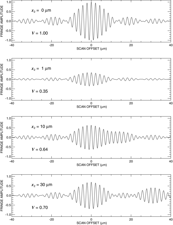
Figure 2. A series of combined fringe patterns for an assumed flux ratio of f2/f1 = 0.5 and a projected separation of zero (upper panel), 1 μm (second panel from the top), 10 μm (third panel from the top), and 30 μm (bottom panel). The 30 μm separation would correspond to a projected angular separation of 20.6 mas for a 300 m baseline (see Equation (4)).
Download figure:
Standard image High-resolution imageWe show in Figure 3 the net visibility that would be measured as a function of projected separation x2. This shows that in general the observed visibility will be less than that of a single star. As expected, for very close separations the visibility varies cosinusoidally with x2 with a frequency of 2π/λ. On the other hand, for projected separations larger than the coherence length ∧coh, the visibility approaches the value 1/(1 + f2/f1) equal to the semiamplitude of the flux diluted fringe pattern of the target.
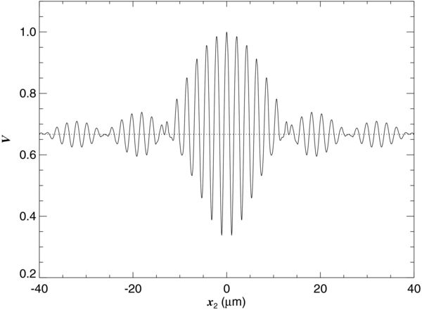
Figure 3. The net visibility as a function of the binary projected separation x2 for the fringe patterns shown in Figure 2.
Download figure:
Standard image High-resolution imageNow suppose that star 1 is a Be star with a disk that is partially resolved, so that if it were observed alone, it would show a visibility V = Vc < 1. Consequently, its fringe pattern would have an semiamplitude given by Vc/(1 + f2/f1). We show a selection of model binary fringe patterns in Figure 4 again for f2/f1 = 0.5 and a specific separation of x2 = 10 μm. The panels show from top to bottom the progressive appearance of the combined fringe patterns as Vc drops from 1 to 0.25. Now the visibility drops in tandem until Vc = 0.50 where the maximum and minimum are set by the fringe pattern of the companion. We show the relationship between the Be star visibility Vc and the net observed visibility Vo in Figure 5 (solid line for x2 = 10 μm). At this separation, there is some slight destructive interference between the fringe patterns that decreases the maximum amplitude for star 2, and as Vc declines to zero, the net visibility attains the amplitude of star 2 alone (f2/f1)/(1 + f2/f1). Figure 5 also shows the (Vc, Vo) relationship for two other separations. The dotted line shows the case of zero separation for maximum constructive interference, and here the visibility declines linearly to (f2/f1)/(1 + f2/f1) as Vc tends to zero. Finally, the dashed line shows the case for a very large separation in which the fringe pattern of star 2 falls beyond the recorded portion of the scan. Here the visibility starts at its diluted value of 1/(1 + f2/f1) at Vc = 1 and declines to near zero at Vc = 0.
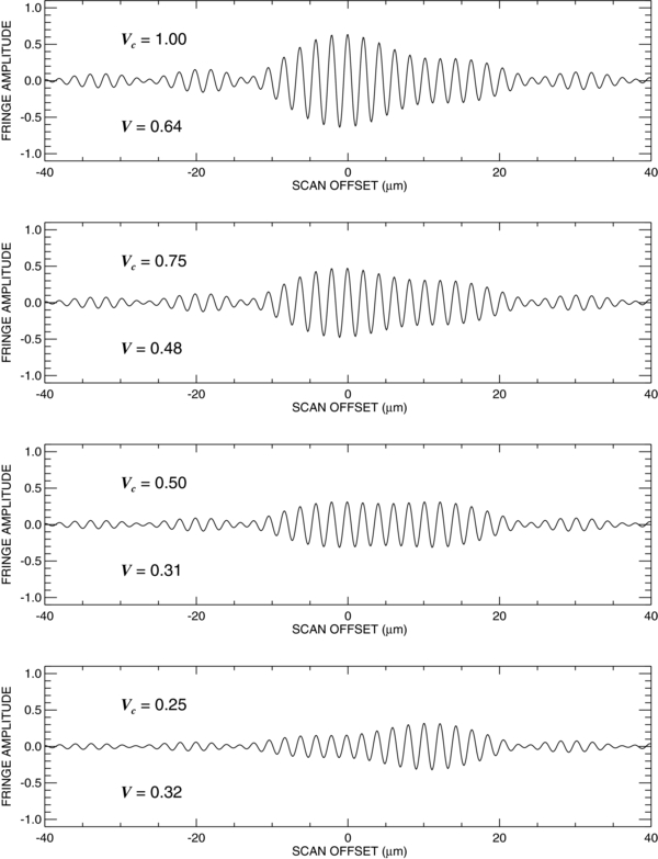
Figure 4. Model binary fringe patterns for f2/f1 = 0.5 and a separation of 10 μm. From top to bottom, the panels show the progressive appearance of the combined fringe patterns as the visibility of a star-plus-disk Vc drops from 1 to 0.25.
Download figure:
Standard image High-resolution image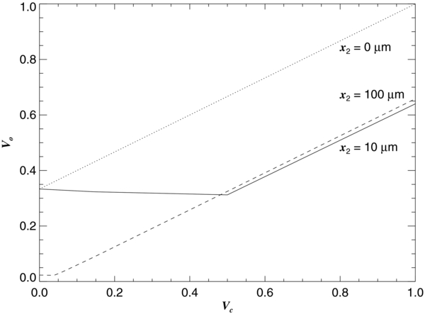
Figure 5. The relationship between the Be star visibility Vc and the net observed visibility Vo. The various lines show the predictions for three binary separation values x2 (see Figure 4 for the x2 = 10 μm case).
Download figure:
Standard image High-resolution imageThus, to correct the observed visibilities for the presence of a companion, we need a diagram like Figure 5 for each observation of a target. We calculated the projected separation of the stars at the time of the observation from the dot product of the relative position vector (from the angular orbital elements given in Table 5) and the (u, v) spatial frequencies for the baseline used. Then we created an associated (Vc, Vo) diagram for each observation based upon the projected separation and effective flux ratio. The corrected visibility Vc was then found by interpolating in the relationship at the observed Vo value. In some rare circumstances, we encountered a double-valued (Vo, Vc) relation, so no correction was attempted because of this ambiguity.
3.4. Fringe Visibility for Be Stars in Multiple Systems
There are six systems in our sample with two or more close companions. Both companions of HD 5394 (γ Cas) are faint, so no correction was made. In the cases of HD 23862 (Pleione) and HD 200120 (59 Cyg), the inner companion is very faint, so corrections were made for only the outer, brighter companion. The spectroscopic pair that comprises the B component of HD 4180 (o Cas) has such a small angular semimajor axis that it was treated as a single object, and thus this system was also corrected as a binary star (Section 3.3). This left two systems, HD 198183 (the triple λ Cyg) and HD 217675 (the quadruple o And), that required corrections for the flux of additional components. The very close B pair of o And was regarded as a single object (see the Appendix), so both λ Cyg and o And were treated as triple star systems.
We made visibility corrections for these two systems in much the same way as for the binaries, except in this case the fringe normalizations were assigned by
Again, we formed model visibilities from the coaddition of the fringe patterns, determined the (Vc, Vo) relationships for the time and baseline configuration of each observation, and then used the inverted relation (Vo, Vc) to determine the corrected visibility.
Unfortunately, there are significant uncertainties surrounding both the magnitude differences and orbital elements for the companions of HD 198183 and HD 217675, and these introduce corresponding uncertainties in the amounts of visibility correction. Our results on these two systems must therefore be regarded as representative visibility solutions rather than definitive ones. However, the corrected interferometry visibilities are all close to one for these two Be stars, which suggests that their disks are only marginally resolved if at all. On the other hand, the much lower uncorrected visibilities of these two show that the influence of the companions is clearly present. Both targets will be important subjects for future, multiple baseline observations with the CHARA Array to determine their orbital properties.
3.5. K-band Magnitude Difference
Our visibility correction procedure requires a knowledge of both the projected separation of the stars (Section 3.2) and their monochromatic flux ratio. Unfortunately, the magnitude differences between the Be star primary and the companion are generally available only in the V-band, and we need to estimate the magnitude differences in the K-band. We must consider the color difference between the components and how much brighter the Be star plus disk appears in the K-band compared to the V-band. The predicted magnitude difference is given by
where F2, F1, andFd are the monochromatic K-band fluxes for the Be companion, the Be star, and the Be disk, respectively. We can estimate the first term from the color differences of the Be star and companion using

where we will assume that the disk contribution is negligible in the V-band so that ▵Vbin = ▵Vobs. In the absence of other information, we estimated the color differences (V − K) by assuming that both the Be star and companion are main-sequence objects, and we used the relationship between (V − K) and magnitude difference from a primary star of effective temperature Teff(Be) (Frémat et al. 2005) for main-sequence stars from Lejeune & Schaerer (2001) to find (V − K) for both stars.
We determined the infrared flux excess term (1 + Fd/F1) from our observed estimate of E⋆(V⋆ − K) (Touhami et al. 2011), which are related by
where the superscripts indicate the filter band. If we assume that the disk contributes no flux in the V-band, then we can rearrange this equation to find the K-band flux excess relative to that of the Be star alone. Then we can combine the results from the two equations above to predict the observed K-band magnitude difference
Our estimates for ▵Kobs are listed in Tables 4 and 5. Note that there are several instances where we give a range for the magnitude difference; these are Be stars that are single-lined spectroscopic binaries with a companion of an unknown type. We consider two hypothetical cases. First, we assume that the companion is a main-sequence star of one solar mass, and we use the Lejeune & Schaerer (2001) main-sequence relation to obtain the magnitude and color differences of the companion. The second case is to assume that the companion is a hot subdwarf (similar to the case of ϕ Per; see Gies et al. 1998) with a typical effective temperature of 30 kK and a stellar radius of 1 R☉. We then estimate ▵Kobs by adopting the main-sequence radius for the Be star according to its effective temperature and by using the Planck function for both stars in order to estimate the monochromatic K-band flux ratio. Table 4 lists those cases with a hyphen in the ▵K column giving the magnitude difference range between that for a hot subdwarf (smaller) and for a solar-type companion (larger). However, we made no visibility corrections in most of these cases because the nature of the companion is so uncertain (with the exception of ϕ Per where the companion's spectrum was detected and characterized by Gies et al. 1998).
3.6. Seeing and Effective Flux Ratio
The CHARA Classic observations were recorded on a single pixel of the Near Infrared Observer camera (NIRO), and the physical size of the pixel corresponds to a square of dimensions 0.8 × 0.8 arcsec on the sky. The flux of companions with separations small compared to 0.8 arcsec will be more or less completely included in the observations, but the flux of companions with larger separations from the central Be star may be only partially recorded according to the separation and seeing conditions at the time of observation. Therefore, we need to calculate the effective flux ratio of companion to target based upon the relative amounts of flux as recorded by this one pixel.
Seeing is usually computed in real time according to the CHARA tip-tilt measurements of the V-band flux of the targets. By assuming that the K-band seeing varies with wavelength by λ−1/5 (Young 1974), the K-band seeing disk is about ∼0.76 times that in V. The effective flux ratio is given by

where I1 and I2 are the net intensity contributions of the primary and secondary component, respectively, recorded by the pixel. We assume a Gaussian profile for the point-spread function as projected on the detector,
where (x0, y0) are the coordinates of the central position of the star on the detector chip, and σ is related to the seeing (σ = 2.355−1θseeing). The intensity distributions of the primary and the secondary components integrated over one pixel on the detector are given by
where ρ is the separation of the binary, and Q is the actual ratio of primary to secondary flux, which is derived from the magnitude difference of the two components in the K-band,

3.7. Visibility Corrections and Their Uncertainties
We used the visibility correction scheme described in Sections 3.3 and 3.4 with the predicted projected angular separation (from the orbital elements in Table 5 and the observed (u, v) spatial frequencies in Table 3) and the effective flux ratio (Sections 3.5 and 3.6) to derive estimates of the Be star visibility alone. The corrected visibilities and their corresponding uncertainties are listed in the last two columns of Table 3 for the nine cases with significant companions. These uncertainties do not include the contributions to the error budget from uncertainties in projected separation and flux ratio. In most cases the projected separations are much larger than the coherence length (typically 9 to 27 mas for 300 m to 100 m baselines), which corresponds to the separated fringe packet case (see lower panel of Figure 2). Thus, the correction depends mainly on the flux dilution term, 1/(1 + f2/f1), and typical uncertainties of 0.2 mag for ▵Kobs only amount to correction uncertainties of ≈0.02 in visibility, i.e., generally smaller than the measurement errors. On the other hand, binaries with projected separations less than the coherence length (mainly observations of o Cas and ϕ Per; see Table 5) have corrections that reflect the fringe amplitude oscillation caused by beating between the fringe patterns of the components (Figure 3). These corrections may amount to (f2/f1)/(1 + f2/f1) in visibility, ≈0.10 for the relatively faint companions considered here. Figure 3 shows that the full range of the correction varies over a projected separation difference of ▵x2 = λ/2, which corresponds to a projected angular separation difference of approximately 0.7 to 2.2 mas for 300 m and 100 m baselines, respectively. The predictive accuracy of the orbital separation probably has comparable uncertainties for the cases of o Cas and ϕ Per, so it is possible that the uncertainties in the corrections may be similar to the corrections themselves in these close separation instances. Nevertheless, we found that implementing the corrections even in these close cases tended to reduce the scatter in the fit of the Be disk visibilities (Section 5.1), so we will adopt the corrected visibilities in the subsequent analysis of all nine targets with significant companions.
4. SPECTRAL ENERGY DISTRIBUTIONS
The SEDs of our sample stars can help us to estimate the photospheric angular diameter of the Be star and the IR flux excess (from a comparison of the observed and extrapolated stellar IR fluxes). The observed IR flux excess can thus be directly compared with the disk flux fraction derived from fits of the visibility measurements. One difficulty with this approach is that the IR flux excess is usually derived assuming that the disk contributes no flux in the optical range, so the stellar SED can be normalized to the optical flux. However, this may lead to an underestimate of the IR excess if the disk flux emission is significant in the optical, which may be the case for stars with dense and large circumstellar disks. The disk flux fraction declines at lower wavelength because of the drop in free–free opacity, and the disk contribution is negligible in the ultraviolet (UV) part of the spectrum. Therefore, we decided to make fits of the UV flux to set the photospheric flux normalization, which will provide a more reliable estimate of the IR flux excess.
We collected UV spectra for all our targets from the archive of the International Ultraviolet Explorer (IUE) satellite, maintained at the NASA Mikulski Archive for Space Telescopes at STScI.7 In most cases, we used the available low dispersion, SWP (1150–1900 Å) and LWP/LWR (1800–3300 Å) spectra, and in cases where there were fewer than two each of these, we used high-dispersion spectra for these two spectral ranges. In the case of HD 217891, all but one of the spectra were made with the small aperture, so we formed an average spectrum and rescaled the flux to that measured by the TD-1 satellite (Thompson et al. 1978). In the case of HD 203467, there were no long-wavelength spectra available in the IUE archive, so we used a combination of IUE SWP spectra (1150–1900 Å), SKYLAB objective-prism spectrophotometry (1900–2300 Å; Henize et al. 1979), and OAO-2 spectral scans (2300–3200 Å; Meade & Code 1980). Fluxes from each spectrum were averaged into 10 Å bins from 1155 to 3195 Å, and then the fluxes from all the available spectra for a given target were averaged at each point in this wavelength grid.
We created model spectra to compare with the IUE observations by interpolating in the grid of model LTE spectra obtained from R. Kurucz. These models were calculated for solar abundances and a microturbulent velocity of 2 km s−1. The interpolation was made in effective temperature and gravity using estimates for these parameters (see Table 1) from the Be star compilation of Frémat et al. (2005). For those sample stars in binaries, we formed a composite model spectrum by adding a model spectrum for each companion that was scaled according to the K-band magnitude difference listed in Table 5.
We then made a nonlinear, least-squares fit of the observed UV spectrum with a model spectrum transformed according to the extinction curve of Fitzpatrick (1999) and normalized by the stellar, limb-darkened angular diameter θLD, and we assumed a standard ratio of total to selective extinction of R = 3.1 for the interstellar extinction curve. Finally, we considered an extension of the fitted photospheric SED into the K-band, and we determined an IR flux excess from
where the monochromatic K-band fluxes are F1 for the Be star component, Ftot for the sum of the photospheric fluxes of the Be and all companions (if any), and Fobs is the observed flux from 2MASS (Cohen et al. 2003; Cutri et al. 2003).
Our results are listed in Table 6 that gives the HD number of the star, the derived reddening E(B − V) and its uncertainty, the limb-darkened stellar angular diameter θs and its uncertainty, and the infrared excess from the disk E⋆(UV − K) and its uncertainty. The final columns list the photospheric fraction of flux cp and its uncertainty that are related to the IR flux excess by

Our derived interstellar reddening values are generally smaller than those derived from the optical colors because the disk flux contribution increases with increasing wavelength through the optical band which mimics interstellar reddening (Dougherty et al. 1994). Furthermore, our derived angular diameters may be smaller in some cases from previous estimates because of the neglect of the flux of the companions in earlier work. Note that we have neglected the effects of rotation (oblateness and gravity darkening) on the SED, and these may influence the flux normalization (Frémat et al. 2005).
5. GAUSSIAN ELLIPTICAL FITS
5.1. Method
Here we show how we can use the interferometric visibility measurements to estimate the stellar and disk flux contributions and to determine the spatial properties of the disk emission component. We used a two-component geometrical disk model to fit the CHARA Classic observations and to measure the characteristic sizes of the circumstellar disks. The model consists of a small uniform disk representing the central Be star and an elliptical Gaussian component representing the circumstellar disk (Quirrenbach et al. 1997; Tycner et al. 2004). Because the Fourier transform function is additive, the total visibility of the system is the sum of the visibility function of the central star and the disk,

where Vtot, Vs, and Vd are the total, stellar, and disk visibilities, respectively, and cp is the ratio of the photospheric flux contribution to the total flux of the system. The visibility for a uniform disk star of angular diameter θs is

where J1 is the first-order Bessel function of the first kind and x is the spatial frequency of the interferometric observation,  . The central Be star is usually mostly unresolved even at the longest baseline of the interferometer, which brings its visibility close to unity, Vs ≃ 1. The disk visibility is given by a Gaussian elliptical distribution
where θmaj is the full width at half-maximum (FWHM) of the spatial Gaussian distribution along the major axis and s is given by

where r is the axial ratio and P.A. is the position angle of the disk major axis. Thus, the Gaussian elliptical model has four free parameters: the photospheric contribution cp, the axial ratio r, the position angle P.A., and the disk angular size θmaj.
5.2. The Effective Baseline
The brightness distribution of the disk projected onto the sky is a function of the inclination and position angle of the major axis. Interferometric observations with a given baseline Bp will sample the disk elliptical distribution according to the angle between the projection of the baseline on the sky and the position angle of the disk major axis. It is helpful to consider rescaling the baseline to account for the changes in the disk size with direction. For a flat disk inclined by an angle i and oriented with the major axis at a position angle P.A. (measured from north to east), we can rescale using the effective baseline Beff (Tannirkulam et al. 2008)
where ϕobs is the baseline position angle at the time of the observations. This new quantity, the effective baseline, takes into consideration the decrease in the interferometric resolution due to the inclination of the disk in the sky, and thus for the purposes of analysis, it transforms the projected brightness distribution of the disk into a nearly circularly symmetric brightness distribution. Thus, the disk part of the visibility can be considered as a function of Beff alone, and below we will use this parameter to present the interferometric results. However, if there is also a stellar flux contribution, than its projection and visibility will be a function of the projected baseline Bp only (if the star appears spherical in the sky). Consequently, models with both stellar and disk contributions should be presented for both the major and minor axis directions in order to show the range in visibility with baseline direction in a single plot. Along the minor axis, for example, ϕobs − P.A. = 90°, so that the relation becomes Beff = Bpcos i, and consequently for edge-on systems with i ∼ 90° a given Beff may correspond to a Bp far larger than available with the Array. Such observations (if possible) would start to resolve the stellar disk and lead to low net visibility (see the dotted line in Figure 8.3).
5.3. Model Degeneracy
The simple geometrical representation of the Be star system may in some cases present a solution family or degeneracy that exists between two fundamental parameters of the Gaussian elliptical model: the Gaussian FWHM θmaj and the stellar photospheric contribution cp. In order to explain the ambiguity in the model, we consider the case of a locus of (cp, θmaj) that produces the same visibility measurement at a particular baseline. We illustrate this relation in Figure 6, which shows an example of a series of (cp, θmaj) Gaussian elliptical visibility curves that all produce a visibility point V = 0.8 at a projected baseline of 200 m (for λ = 2.1329 μm and a Be star angular diameter θUD = 0.3 mas). The plot shows models for (cp, θmaj) = (0.156, 0.6 mas) (solid line), (cp, θmaj) = (0.719, 1.2 mas) (dotted line), and (cp, θmaj) = (0.816, 2.4 mas) (dashed line). Figure 7 shows the relationship between the Gaussian elliptical FWHM and the stellar photospheric contribution for the family of curves that go through the observed point V = 0.8 at a 200 m baseline. Larger circumstellar disks are associated with larger stellar flux contributions, and vice versa, which demonstrates that a single interferometric measurement does not discriminate between a bright small disk and a large faint one. Additional measurements at different baselines are necessary to resolve this ambiguity.
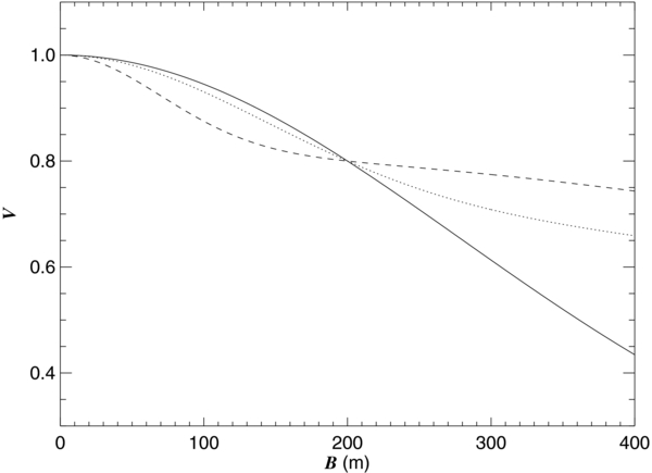
Figure 6. A set of three Gaussian elliptical models of different (cp, θmaj) that produce a visibility point V = 0.8 at a 200 m projected baseline. The solid curve is for (cp, θmaj) = (0.156, 0.6 mas), the dotted curve is for (cp, θmaj) = (0.719, 1.2 mas), and the dashed curve is for (cp, θmaj) = (0.816, 2.4 mas).
Download figure:
Standard image High-resolution image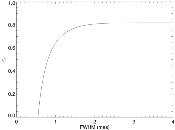
Figure 7. The relation between cp and θmaj = FWHM for Gaussian elliptical visibility models that go through the same observed point of V = 0.8 at a 200 m baseline.
Download figure:
Standard image High-resolution imageNote that if the interferometric observations are all located on one projected baseline in the (u, v) plane, then the disk properties are defined in only one dimension. Thus, in such circumstances it is not possible to estimate the axial ratio r or the position angle of the disk major axis P.A. Only a lower limit for θmaj can be set in such cases.
5.4. Fitting Results
The circumstellar disk is modeled with a Gaussian elliptical flux distribution centered on the Be star. This disk model has four independent parameters (r, P.A., cp, θmaj), and one assumed parameter, the stellar diameter θs (Table 6). The fitting procedure consists of solving for the model parameters using the IDL nonlinear least-squares curve fitting routine MPFIT (Markwardt 2009), which provides a robust way to perform multi-parameter surface fitting. Model parameters can be fixed or free depending on the (u, v) distribution of the observations.
For the cases with limited coverage in the (u, v) plane, setting some model parameters to fixed values was necessary in order to successfully fit the data. We adopted additional constraints on some model parameters that are well defined from studies such as inclination estimates from Frémat et al. (2005) and intrinsic polarization angles from McDavid (1999) and Yudin (2001). Also, we occasionally used values of the IR flux excess derived from the SEDs of Be stars to estimate the stellar photospheric contribution cp when needed.
Our fitting results are summarized in Table 7, where the cases with a fixed parameter are identified by a zero value assigned to its corresponding uncertainty. Column 1 of Table 7 lists the HD number of the star, Columns 2 and 3 list the axial ratio r and its uncertainty, Columns 4 and 5 list the disk position angle along the major axis P.A. and its uncertainty, Columns 6 and 7 list the photospheric contribution cp and its uncertainty, Columns 8 and 9 list the angular FWHM of the disk major axis θmaj and its uncertainty, Column 10 lists the reduced  of the fit, Columns 11 and 12 list the corrected photospheric contribution cp(corr) and its uncertainty (see Section 5.5), respectively, Columns 13 and 14 list the disk-to-star radius ratio Rd/Rs and its uncertainty, and finally, Column 15 indicates the cases of fully resolved disks (Y), marginally resolved disks (M), and unresolved disks (N) in our Be star sample.
Table 7. Gaussian Elliptical Fits of the Interferometric Visibilities
| HD | r | δra | P.A. | δP.A.a | cp | δcpa | θmaj | δθmaj |  |
cp(corr) | δcp(corr) | Rd/Rs | δRd/Rs | Res. |
|---|---|---|---|---|---|---|---|---|---|---|---|---|---|---|
| Number | (°) | (°) | (mas) | (mas) | ||||||||||
| (1) | (2) | (3) | (4) | (5) | (6) | (7) | (8) | (9) | (10) | (11) | (12) | (13) | (14) | (15) |
| HD 004180 | 0.583 | 0.101 | 101.4 | 13.8 | 0.500 | 0.000 | 1.027 | 0.173 | 3.03 | 0.558 | 0.019 | 3.243 | 0.493 | Y |
| HD 005394 | 0.722 | 0.038 | 38.2 | 5.0 | 0.082 | 0.036 | 1.236 | 0.063 | 15.63 | 0.190 | 0.032 | 2.946 | 0.134 | Y |
| HD 010516 | 0.100 | 0.000 | 135.5 | 3.5 | 0.682 | 0.017 | 2.441 | 0.198 | 8.18 | 0.700 | 0.016 | 10.437 | 0.838 | Y |
| HD 022192 | 0.251 | 0.562 | 136.8 | 4.5 | 0.518 | 0.000 | 1.030 | 0.264 | 1.50 | 0.612 | 0.090 | 3.502 | 0.898 | Y |
| HD 023630 | 1.000 | 0.000 | 00.0 | 0.0 | 0.448 | 0.297 | 0.091 | 0.000 | 5.85 | 1.000 | 0.000 | 1.010 | 0.000 | N |
| HD 023862 | 0.438 | 0.000 | 159.0 | 0.0 | 0.500 | 0.000 | 0.364 | 0.220 | 3.33 | 0.715 | 0.057 | 1.879 | 2.315 | M |
| HD 025940 | 0.866 | 0.000 | 108.0 | 0.0 | 0.412 | 0.000 | 0.597 | 0.245 | 2.55 | 0.539 | 0.009 | 2.072 | 0.676 | Y |
| HD 037202 | 0.148 | 0.027 | 125.4 | 1.3 | 0.422 | 0.016 | 1.790 | 0.073 | 4.30 | 0.534 | 0.013 | 4.146 | 0.159 | Y |
| HD 058715 | 0.783 | 0.000 | 139.5 | 0.0 | 0.717 | 0.000 | 0.777 | 0.181 | 2.77 | 0.851 | 0.132 | 1.539 | 0.194 | Y |
| HD 109387 | 1.000 | 0.000 | 0.0 | 0.0 | 0.803 | 0.025 | 3.214 | 0.749 | 6.36 | 0.805 | 0.025 | 8.407 | 1.932 | Y |
| HD 138749 | 0.200 | 0.000 | 177.0 | 0.0 | 0.500 | 0.000 | 0.261 | 0.177 | 2.06 | 0.907 | 0.056 | 1.332 | 0.470 | N |
| HD 142926 | 0.270 | 0.082 | 98.4 | 5.7 | 0.822 | 0.000 | 1.329 | 0.714 | 0.51 | 0.830 | 0.005 | 7.330 | 3.824 | M |
| HD 142983 | 0.405 | 0.000 | 50.0 | 0.0 | 0.242 | 0.000 | 0.836 | 0.164 | 0.75 | 0.294 | 0.005 | 4.963 | 0.936 | Y |
| HD 148184 | 0.947 | 0.000 | 20.0 | 0.0 | 0.123 | 0.000 | 0.858 | 0.142 | 1.59 | 0.157 | 0.004 | 4.385 | 0.690 | Y |
| HD 164284 | 0.685 | 0.000 | 18.0 | 0.0 | 0.728 | 0.000 | 0.892 | 0.187 | 2.92 | 0.739 | 0.005 | 5.082 | 1.025 | M |
| HD 166014 | 0.435 | 0.279 | 67.8 | 32.5 | 0.250 | 0.000 | 0.337 | 0.105 | 1.88 | 0.941 | 0.069 | 1.191 | 0.108 | M |
| HD 198183 | 0.826 | 0.000 | 30.0 | 0.0 | 0.133 | 0.000 | 0.163 | 0.198 | 4.91 | 0.749 | 0.177 | 1.292 | 0.779 | N |
| HD 200120 | 0.310 | 0.000 | 95.0 | 0.0 | 0.143 | 0.000 | 0.554 | 0.190 | 4.67 | 0.264 | 0.023 | 3.852 | 1.219 | M |
| HD 202904 | 0.258 | 0.129 | 108.8 | 2.9 | 0.541 | 0.370 | 1.211 | 0.786 | 1.75 | 0.604 | 0.319 | 4.225 | 2.544 | Y |
| HD 203467 | 0.799 | 0.000 | 76.0 | 0.0 | 0.343 | 0.000 | 0.528 | 0.087 | 1.62 | 0.418 | 0.006 | 2.861 | 0.415 | Y |
| HD 209409 | 0.249 | 0.059 | 107.5 | 2.2 | 0.617 | 0.000 | 1.525 | 0.642 | 1.80 | 0.647 | 0.006 | 5.776 | 2.374 | Y |
| HD 212076 | 0.955 | 0.000 | 148.0 | 0.0 | 0.308 | 0.000 | 0.295 | 0.044 | 1.61 | 0.487 | 0.032 | 1.852 | 0.202 | M |
| HD 217675 | 0.022 | 0.000 | 25.0 | 0.0 | 0.340 | 0.195 | 0.056 | 0.000 | 2.23 | 1.000 | 0.000 | 1.010 | 0.000 | N |
| HD 217891 | 0.702 | 0.150 | 30.6 | 17.1 | 0.692 | 0.309 | 0.804 | 0.593 | 1.81 | 0.722 | 0.279 | 3.261 | 2.098 | Y |
Note. aUncertainty of zero indicates cases where the model parameter was fixed in advance of the fit.
Download table as: ASCIITypeset image
Plots of the best-fit solutions showing the visibility curves of the system disk-plus-star as a function of the effective baseline in meters along with our interferometric data are presented in Figure 8. The solid lines in Figure 8 represent the best-fit visibility model of the disk along the major axis, the dotted lines represent the best-fit visibility model of the disk along the minor axis, and the star signs represent the interferometric data.
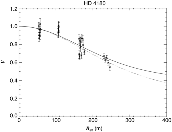
Figure 8.
Calibrated visibilities vs. the effective baseline. The solid line and the dotted lines represent the Gaussian elliptical model along the major and minor axes, respectively, and the star signs represent the interferometric data. (The complete figure set (24 images) is available in the online journal.)
Download figure:
Standard image High-resolution imageWe find that the circumstellar disks of the four Be stars, HD 23630, HD 138749, HD 198183, and HD 217675 were unresolved at the time of our CHARA Array observations, while the circumstellar disks of HD 23862, HD 142926, HD 164284, HD 166014, HD 200120, and HD 212076 were only marginally resolved. Those are the cases where we had to fix r, P.A., and/or cp in order to make Gaussian elliptical model fits to the data. On the other hand, we successfully resolved the circumstellar disks around the other 14 Be stars and were able to perform four-parameter Gaussian elliptical fits for most of them as listed in Table 7.
5.5. Corrections to the Gaussian Model
Modeling a circumstellar disk with an elliptical Gaussian intensity distribution is convenient but not completely realistic. The flux distribution in the model assumes that light components from the circumstellar disk and the central star are summed and that no mutual obscuration occurs. It is important to note that in the case of small disks most of the model disk flux is spatially coincident with the photosphere of the star, so the assignment of the flux components becomes biased.
To illustrate this effect, we show in Figure 9 the model components for a case with a faint disk. The dotted line in Figure 9 shows the assumed form of the intensity of the uniform disk of the star (angular diameter of 0.68 mas), the dashed line shows the Gaussian distribution of the circumstellar disk along the projected major axis (FWHM = 0.55 mas), and the solid line shows the sum of the two intensity components. In the case where the FWHM of the circumstellar emission is similar to or smaller than the stellar diameter, most of the disk flux occurs over the stellar photosphere where the sum produces a distribution similar to that of a limb-darkened star.

Figure 9. A set of intensity profiles for a faint disk case. The diagram shows the stellar (uniform disk) flux (dotted line), the Gaussian circumstellar disk flux (dashed line), and their sum (upper solid line). In this case the Gaussian FWHM (indicated by the dash-dotted line) is smaller than the stellar diameter, and the revised circumstellar disk radius (from Equation (21)) is shown as lower solid line on the right side.
Download figure:
Standard image High-resolution imageThe interpretation of the results obtained from the Gaussian elliptical fits must be regarded with caution in situations where the derived disk radius is smaller than the star's radius and a significant fraction of the disk flux is spatially coincident with that of the star. Consequently, we decided to correct the Gaussian elliptical fitting results in two ways. First, the disk radius was set based upon the relative intensity decline from the stellar radius, and we adopted the disk radius to be that distance where the Gaussian light distribution along the major axis has declined to half its value at the stellar equator. The resulting ratio of disk radius to star radius is then given by
where θmaj is the Gaussian FWHM along the major axis derived from the fits, and θs is the angular diameter of the central star. Second, the model intensity over the photosphere of the star from both the stellar and disk components was assigned to the flux from the star in an optically thin approximation. The fraction of the disk flux that falls on top of the star is f(1 − cp), where f is found by integrating over the stellar disk the Gaussian spatial distribution given by (Tycner et al. 2004)
where r is the axial ratio and (x, y) are the sky coordinates in the direction of the minor and major axes. Consequently, this fraction of the model disk flux should be reassigned to the star and removed from the disk contribution. Then the revised ratio of total disk to stellar flux is
which is lower than the simple estimate of (1 − cp)/cp. We list in Columns 11–14 of Table 7 the revised values of the stellar flux contribution cp and the Be disk radius Rd/Rs (along with the corresponding uncertainties) obtained by applying this correction using the stellar angular diameters from Table 6.
6. DISCUSSION
6.1. Comparison with Other Results
It is important to validate our results against other published data wherever possible. However, since this is the first large-scale study of the K-band emission of northern Be stars, it is difficult to make direct comparisons. We list in Table 8 the available measurements of Gaussian elliptical model parameters of Be star disks for the stars in our sample (excluding the work of Gies et al. 2007 that is included in our analysis). There is only one other K-band measurement available by Pott et al. (2010), but even in this case a direct comparison of θmaj is difficult because of the different assumptions made about the remaining parameters. Measurements of the disk emission in other bands will likely yield different diameter estimates (Section 6.2). Nevertheless, we can compare our results on the geometry of the disks with previous work, and we can consider the parameter estimates resulting from other kinds of observations.
Table 8. Other Interferometric Results
| HD | r | δr | P.A. | δP.A. | θmaj | δθmaj | Band | Ref. |
|---|---|---|---|---|---|---|---|---|
| Number | (°) | (°) | (mas) | (mas) | ||||
| (1) | (2) | (3) | (4) | (5) | (6) | (7) | (8) | (9) |
| HD 004180 | 1.00 | ⋅⋅⋅ | ⋅⋅⋅ | ⋅⋅⋅ | 1.90 | 0.10 | Hα | 1 |
| HD 005394 | 0.70 | 0.02 | 19 | 2 | 3.47 | 0.02 | Hα | 2 |
| HD 005394 | 0.58 | 0.03 | 31 | 1 | 3.59 | 0.04 | Hα | 3 |
| HD 005394 | 0.74 | 0.05 | 19 | 5 | 0.76 | 0.05 | R | 4 |
| HD 005394 | 0.75 | 0.05 | 12 | 9 | 0.82 | 0.08 | H | 4 |
| HD 010516 | 0.46 | 0.04 | 118 | 5 | 2.67 | 0.20 | Hα | 2 |
| HD 010516 | 0.27 | 0.01 | 119 | 1 | 2.89 | 0.09 | Hα | 3 |
| HD 022192 | 0.47 | 0.11 | 147 | 11 | 3.26 | 0.23 | Hα | 2 |
| HD 022192 | 0.34 | 0.10 | 96 | 2 | 4.00 | 0.20 | Hα | 5 |
| HD 022192 | <0.61 | ⋅⋅⋅ | 158 | 10 | 111.00 | 16.00 | 15 GHz | 6 |
| HD 023630 | 0.95 | 0.22 | 19 | ⋅⋅⋅ | 2.65 | 0.14 | Hα | 2 |
| HD 023630 | 0.75 | 0.05 | 45 | 9 | 2.08 | 0.18 | Hα | 7 |
| HD 025940 | 0.89 | 0.13 | 68 | ⋅⋅⋅ | 2.77 | 0.56 | Hα | 2 |
| HD 025940 | 0.77 | 0.10 | 115 | 33 | 2.10 | 0.20 | Hα | 5 |
| HD 037202 | 0.28 | 0.02 | 122 | 4 | 4.53 | 0.52 | Hα | 2 |
| HD 037202 | 0.31 | 0.07 | 118 | 4 | 3.14 | 0.21 | Hα | 8 |
| HD 037202 | 0.24 | 0.14 | 123 | 6 | 1.57 | 0.28 | H | 9 |
| HD 037202 | ⋅⋅⋅ | ⋅⋅⋅ | 126 | 2 | ⋅⋅⋅ | ⋅⋅⋅ | Brγ | 10 |
| HD 058715 | ⋅⋅⋅ | ⋅⋅⋅ | ⋅⋅⋅ | ⋅⋅⋅ | 2.65 | 0.10 | Hα | 2 |
| HD 058715 | 0.69 | 0.15 | 40 | 30 | 2.13 | 0.50 | Hα | 7 |
| HD 058715 | 0.76 | 0.10 | 140 | 6 | 0.33 | 0.18 | H | 10 |
| HD 109387 | 1.00 | ⋅⋅⋅ | ⋅⋅⋅ | ⋅⋅⋅ | 2.00 | 0.30 | Hα | 11 |
| HD 142983 | 0.60 | 0.11 | 50 | 9 | 1.72 | 0.20 | H | 12 |
| HD 142983 | ⋅⋅⋅ | ⋅⋅⋅ | 50 | ⋅⋅⋅ | 1.65 | 0.05 | K | 13 |
| HD 148184 | 1.00 | ⋅⋅⋅ | ⋅⋅⋅ | ⋅⋅⋅ | 3.46 | 0.07 | Hα | 14 |
| HD 202904 | 1.00 | ⋅⋅⋅ | ⋅⋅⋅ | ⋅⋅⋅ | 1.00 | 0.20 | Hα | 11 |
| HD 217891 | 1.00 | ⋅⋅⋅ | ⋅⋅⋅ | ⋅⋅⋅ | 2.40 | 0.20 | Hα | 11 |
References. (1) Koubský et al. 2010; (2) Quirrenbach et al. 1997; (3) Tycner et al. 2006; (4) Stee et al. 2012; (5) Delaa et al. 2011; (6) Dougherty & Taylor 1992; (7) Tycner et al. 2005; (8) Tycner et al. 2004; (9) Schaefer et al. 2010; (10) Kraus et al. 2012; (11) C. Tycner, private communication; (12) Štefl et al. 2012; (13) Pott et al. 2010; (14) Tycner et al. 2008.
Download table as: ASCIITypeset image
We begin by comparing the stellar and disk flux contributions that we derived from the Gaussian elliptical fits (Table 7) with those estimated from the IR-excess in the SEDs (Table 6). Among the 14 stars in our sample with reliable detections of disk emission, we fit for the stellar flux contribution in six cases. The corrected parameter cp(corr) = Fs/(Fs + Fd) is plotted together with the SED estimate of this ratio in Figure 10. The uncertainties are significant, but these two estimates of stellar flux in the K-band appear to be consistent (perhaps surprisingly so, because of the known temporal flux variations and large time span between the 2MASS photometry and our interferometric observations).
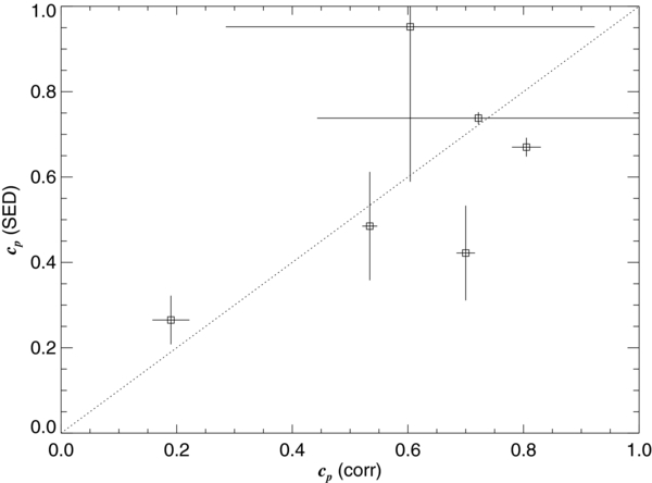
Figure 10. A comparison between the values of the K-band photospheric contribution cp(SED) derived from the SED fits and those from the Gaussian elliptical fits cp(corr).
Download figure:
Standard image High-resolution imageNext we consider the disk axial ratio r that is related approximately to the disk normal inclination i by (Grundstrom & Gies 2006)

where the second term accounts for the increase in the minor axis size caused by the increase in disk thickness with radius. We expect that the disk inclination will be the same as the stellar spin inclination because the disk is probably fed by equatorial mass loss. Frémat et al. (2005) estimated the stellar inclinations for most of our targets by comparing the projected rotational velocity Vsin i with the critical rotational velocity Vcrit, for which the equatorial centripetal and gravitational accelerations balance, and by assuming that Be stars as a class share a common ratio of angular rotational to critical velocity. The axial ratios derived from their estimates of spin inclination are given in the final column of Table 1. There are seven targets with fitted estimates of r among our 14 reliable detections, and we plot these values together with r(i) from the inclinations from Frémat et al. (2005) in Figure 11 (indicated by square symbols). Figure 11 includes other r estimates from previous interferometry (Table 8). With two exceptions ( Cyg = HD 202904 above and γ Cas = HD 5394 below), the estimates from interferometry and rotational line broadening are in broad agreement. Three of our targets have prior interferometric estimates of r, and our results agree within the uncertainties. Note that the increase in disk thickness with radius implies that r will appear larger in bands where the disk emission extends to larger radius (Hα), and in two cases (ψ Per = HD 22192 and ζ Tau = HD 37202) r(Hα) is larger than r(K-band), while they are the same in the third case (γ Cas = HD 5394).
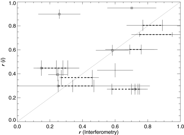
Figure 11. A comparison between the values of the disk axial ratio r(i) adopted from the stellar inclinations given by Frémat et al. (2005) and those derived from interferometry (our estimates are indicated by square symbols while the rest are from prior work listed in Table 8). Thick dashed lines connect the various estimates from interferometry for the same star.
Download figure:
Standard image High-resolution imageThe disk normal is expected to have the same position angle in the sky as that for the intrinsic polarization (from scattering in the inner disk; Quirrenbach et al. 1997). We show in Figure 12 a comparison of the position angles derived from interferometry with those from polarimetric studies (McDavid 1999; Yudin 2001). These generally agree within the uncertainties, but there are some exceptions ( Cyg = HD 202904 and several cases with large axial ratio r where it is difficult to determine position angle). Our results are fully consistent for four targets with previous interferometric estimates of P.A. All these comparisons lend support to our strategy of fixing the cp, r, and P.A. parameters in those cases where there were ambiguities with the full four-parameter, Gaussian elliptical fit.
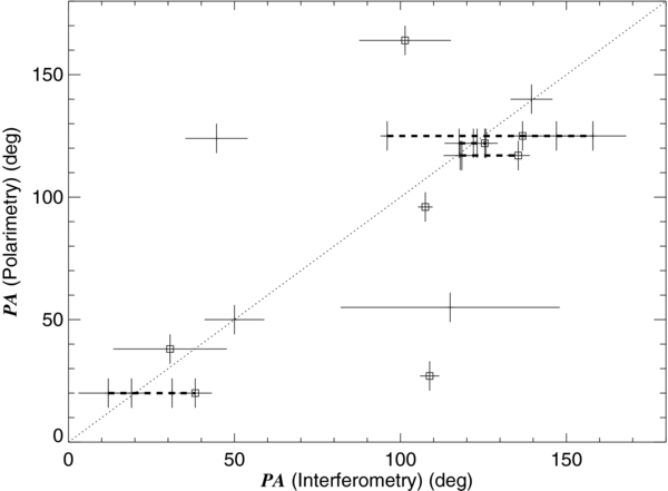
Figure 12. A comparison between the values of the disk long axis position angle P.A. adopted from the intrinsic polarization angle plus 90° (McDavid 1999; Yudin 2001) and those derived from interferometry (our estimates are indicated by square symbols while the rest are from prior work listed in Table 8). Thick dashed lines connect the various estimates from interferometry for the same star.
Download figure:
Standard image High-resolution image6.2. Disk Diameters
We clearly detected the visibility decline due to the disk in 14 stars in our sample. The ratio of disk to stellar radius (Table 7, Column 13) varies from 1.5 to 10 with a mean value of 4.4 among this subsample, but our detections are probably biased toward those cases with larger and brighter disks. We compare these K-band diameters with those measured for Hα (Table 8) in Figure 13, and this demonstrates that in most cases the Hα disk diameters are much larger. Gies et al. (2007) attributed this difference to the larger opacity of Hα compared to the free–free and bound–free opacities that dominate the disk emission in the near-infrared. There are three targets that fall below the trend:  Cyg = HD 202904 (but with an uncertainty that may be consistent with the trend), ϕ Per = HD 10516, and κ Dra = HD 109387. It is curious that the latter two are both short-period binaries, and it may be that the usually larger Hα emitting regions are truncated by tidal forces, so that their K-band and Hα disk sizes are comparable. After setting aside these three discrepant cases, the unweighted slope of the relation starting from an origin at (Rd(K-band)/Rs, Rd(Hα)/Rs) = (1, 1) is ▵Rd(Hα)/▵Rd(K-band) = 4.0 ± 0.5 (s.d. of the mean), and this slope is indicated by a dotted line in Figure 13. Such a correlation is helpful in predicting the size of the circumstellar disk in the K-band from Hα observations, and vice versa, especially since Be star disks are generally highly variable and simultaneous, multi-wavelength observations are usually difficult to obtain.
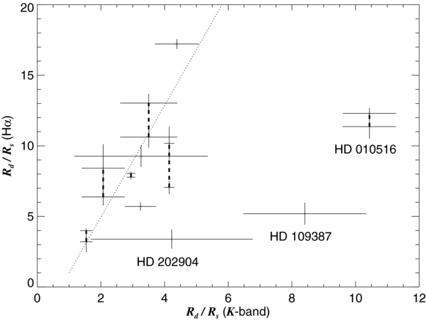
Figure 13. A comparison of the K-band disk sizes with the Hα disk sizes (Rd/Rs = θmaj/θs with θmaj from Table 8 and θs from Table 7). The dotted line represents a linear fit to the data with a slope of 4.0. Thick dashed lines connect multiple Hα measurements for the same star.
Download figure:
Standard image High-resolution imageNext, we consider the connection between disk size and brightness. If the disk gas near the central Be star has a temperature that is some fraction of the stellar temperature, then we might expect to find a correlation between the surface intensity I of the inner disk and star in the limit of high disk optical depth,

for some constant b. We can explore this relationship by considering the Gaussian elliptical model prediction for the disk brightness at the stellar equator (Tycner et al. 2004),
The mean stellar intensity in the model is
Then we can equate these with proportionality constant b to obtain
This relation predicts that the disk to star flux ratio (left-hand side) is approximately proportional to the ratio of disk to star projected area (right-hand side).
The Gaussian elliptical parameters from Table 7 and the stellar angular diameters from Table 6 were used to calculate the terms on both sides of the equation, and they are plotted together in Figure 14 (where we assumed a minimum uncertainty of 5% for those cases where the formal uncertainties may be underestimated). We see that the Be stars with the largest disk to stellar flux ratio are often those with a large ratio of circumstellar to stellar angular diameter. However, a counter example is the case of κ Dra = HD 109387 that is plotted with a large but faint disk (lower right location in Figure 14). The fit of the Gaussian elliptical model parameters in this case is constrained by a set of 100 m baseline measurements from Gies et al. (2007) (see Figure 8.10), and if a fit was made from the new measurements alone, then the disk size would be much smaller (as also suggested by the smaller Hα disk size shown in Figure 13). Given these uncertainties, our measurement for κ Dra may be set aside from consideration here. An unweighted, nonparametric, correlation test for the remaining 13 Be stars yields a Kendall's statistic of τ = 0.205, which has null rejection probability of 37%, i.e., a value which is not small enough to reject with confidence the null hypothesis of no correlation. We suspect that the poor correlation results from a break down among the faint disk stars of our simplifying assumption that the disks are optically thick, which may only be applicable to the brightest disk cases. We show for completeness in Figure 14 a linear fit of the sample of 13 stars that has a constant of proportionality of b = 0.18 ± 0.04 (s.d. of the mean). We caution again that such a relation may only hold for dense, optically thick disks and that our results may be biased against detection of fainter disks in general. We are planning to investigate further the question of disk surface intensity in another paper that will apply physical models and radiative transfer calculations to fit the observed visibilities.
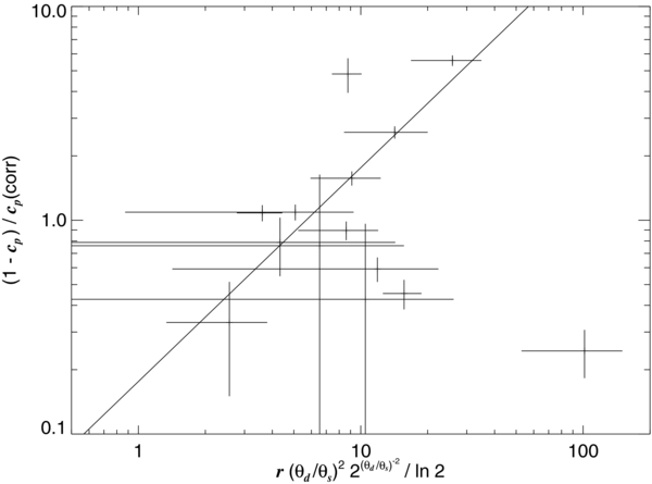
Figure 14. A plot of the approximate disk to star flux ratio Fd/Fs = (1 − cp)/cp(corr) as a function of a product related to the projected disk to stellar area on the sky. A linear relationship (unit slope line) may exist for large optically thick disks. The scatter is largest among faint disk systems (the lower, right point represents κ Dra = HD 109387).
Download figure:
Standard image High-resolution image6.3. Detection Limits
We found that the criterion for a confident detection of the circumstellar disk is usually a decline in visibility below V = 0.8 at the longest baselines available. We can use this criterion to estimate the limitations on disk sizes that we can detect for Be stars at different distances. The visibility measured along baselines aligned with the projected major axis of the disk is a function of the photospheric flux fraction cp, the ratio of disk to stellar radius Rd/Rs, and the stellar angular diameter θs (Equations (17)– (19)). Thus, given Rd/Rs and θs we can find θmaj, and the remaining parameter to estimate is cp. In practice this could be estimated from a simultaneous analysis of the SED of the Be star. However, for our purpose here, we adopted the relationship between the disk to star flux ratio and projected surface areas (Equation (29) and Figure 14) to estimate cp from r and Rd/Rs. This relationship is poorly defined for fainter disks ((1 − cp)/cp < 1), where the disks become optically thin and the ratio of areas argument no longer applies.
The stellar angular diameter is found from the assumed stellar radius and distance, and we made estimates for two cases, B0 V and B8 V types for the Be star, and for three distances corresponding to visual magnitudes 3, 5, and 7. We used stellar radii and absolute magnitudes for these classifications from the compilation of Gray (2005), and we neglected any extinction in the calculation of distance from the magnitude difference. Figure 15 shows the resulting predicted visibilities for a K-band measurement with a projected baseline of 300 m as a function of Rd/Rs for these different cases. Each plot shows how the visibility at this baseline declines as the disk size increases, and we can use these to estimate the smallest disk detectable. For example, we see in Figure 15(a) for a B0 V star of apparent magnitude 5 that the curve dips below V = 0.8 at Rd/Rs = 3.4 from which we would infer that only disks larger than this would be detected with the CHARA Array. As expected, we can detect smaller disks in nearer (brighter) Be stars. Figure 15(b) shows the case for a later B8 V type that is somewhat more favorable for detection of smaller disks. Note that at small disk radii we simply assume that all the flux is stellar, so the limiting visibility near Rd/Rs = 1 corresponds to the stellar visibility.
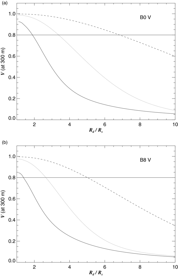
Figure 15. A plot of the expected calibrated visibility measured at a baseline of 300 m for a Be star of type B0 V (a) and B8 V (b) as a function of disk to stellar radius along the major axis. The thick solid, dotted, and dashed lines correspond to predictions for a star of visual magnitude 3, 5, and 7, respectively. The thin horizontal line marks the V = 0.8 criterion, and if the visibility drops below this line then the disk is detected with some confidence.
Download figure:
Standard image High-resolution image
6.4. Rotational and Critical Velocities
Be stars are generally fast rotators, but it is difficult to determine the actual equatorial rotational velocity Vrot from the observed projected rotational velocity Vsin i (measured from the rotational Doppler broadening of the lines; Townsend et al. 2004) because of the unknown stellar inclination i. If we assume that the stellar spin and disk rotational axes are coaligned, then we can use the disk axial ratio to set the stellar inclination (Equation (25)). We collected the seven r values derived from our fits (Table 7) together with estimates from previous work (Table 8) to find mean sin i factors for 12 Be stars in our program. We adopted the projected photospheric rotational velocities Vsin i and the critical rotational velocities Vcrit from Frémat et al. (2005), who derived these values after making corrections for the effects of gravity darkening. Then we divided Vsin i by sin i to find the equatorial rotational velocity Vrot. Our results appear in Table 9 that lists the HD number of the star, Vsin i and Vcrit (Frémat et al. 2005), Vrot, and two ratios, Vrot/Vcrit and Ωrot/Ωcrit. The ratio of angular rotational velocities is given for the Roche approximation using expressions from Ekström et al. (2008),
Table 9. Linear Rotational and Critical Velocities
| HD | Vsin i | Vcrit | Vrot | Vrot/Vcrit | Ωrot/Ωcrit |
|---|---|---|---|---|---|
| Number | (km s−1) | (km s−1) | (km s−1) | ||
| HD 004180 | 208 ± 13 | 332 ± 21 | 249 ± 26 | 0.75 ± 0.09 | 0.91 ± 0.06 |
| HD 005394 | 441 ± 27 | 577 ± 36 | 599 ± 37 | 1.04 ± 0.09 | ≈1 |
| HD 010516 | 462 ± 33 | 590 ± 42 | 487 ± 6 | 0.82 ± 0.06 | 0.96 ± 0.03 |
| HD 022192 | 295 ± 15 | 397 ± 20 | 310 ± 70 | 0.78 ± 0.18 | 0.93 ± 0.11 |
| HD 023630 | 149 ± 8 | 274 ± 15 | 216 ± 20 | 0.79 ± 0.09 | 0.94 ± 0.05 |
| HD 025940 | 220 ± 13 | 386 ± 21 | 323 ± 82 | 0.84 ± 0.22 | 0.96 ± 0.10 |
| HD 037202 | 326 ± 7 | 466 ± 13 | 333 ± 6 | 0.71 ± 0.02 | 0.89 ± 0.02 |
| HD 058715 | 231 ± 14 | 380 ± 24 | 327 ± 91 | 0.86 ± 0.25 | 0.97 ± 0.10 |
| HD 142983 | 407 ± 22 | 501 ± 28 | 484 ± 56 | 0.97 ± 0.12 | 1.00 ± 0.01 |
| HD 202904 | 167 ± 20 | 468 ± 30 | 171 ± 7 | 0.37 ± 0.03 | 0.52 ± 0.04 |
| HD 209409 | 282 ± 20 | 391 ± 27 | 288 ± 4 | 0.74 ± 0.05 | 0.90 ± 0.04 |
| HD 217891 | 100 ± 6 | 367 ± 24 | 135 ± 44 | 0.37 ± 0.12 | 0.53 ± 0.16 |
Download table as: ASCIITypeset image
We find that most of the stars in this subsample are rotating very quickly, and two targets may have attained the critical rate (γ Cas = HD 5394 and 48 Lib = HD 142983). However, there are two targets with much more moderate rotational velocities, β Psc = HD 217891 and  Cyg = HD 202904. The former has a rather large axial ratio r = 0.70 ± 0.15, and it is possible that the uncertainties would allow a small inclination and hence large rotational velocity. However, the case of
  Cyg is more difficult to understand. Neiner et al. (2005) argue on the basis of the narrow lines in the spectrum that the axial ratio should be close to r ≈ 0.9 if it is actually a rapid rotator. This is much larger than the value we derive from the Gaussian elliptical fits, r = 0.26 ± 0.13. Additional interferometric observations are needed to confirm or remove this discrepancy.
We find a mean angular velocity ratio of Ωrot/Ωcrit = 0.88 ± 0.17 (s.d.) for the sample of 12 Be stars or 0.95 ± 0.04 (s.d.) if we remove β Psc and  Cyg from the sample. These results support earlier Be star angular velocity ratio estimates of 0.88 (Frémat et al. 2005), 0.7–1.0 (Cranmer 2005), 0.8–1.0 (Huang et al. 2010), and 0.95 ± 0.02 (Meilland et al. 2012). The consistency of these results suggests that rapid rotation in Be stars plays a key role in the Be phenomenon.
7. CONCLUSIONS
Our CHARA Array interferometric survey of northern sky Be stars has led to the resolution of extended K-band continuum emission from the disks of 14 stars among of our sample of 24 stars. We interpreted the visibility measurements with a simple geometrical model that assumes a Gaussian elliptical brightness distribution for the circumstellar disks. The model fits yield estimates of the disk angular diameter, axial ratio, position angle, and the photospheric and disk flux contributions in the K-band. We demonstrated that the results are consistent with earlier interferometric studies of the disk Hα emission and with other estimates for the disk parameters from spectroscopic and polarimetric studies.
We determined estimates for the stellar angular diameters and infrared flux excesses from fits of the UV and near-infrared SEDs. We find that the mean ratio of the K-band disk to stellar diameter is 4.4 with a range from 1.5 to 10 for the detected cases. The ratio is similar among both early- and late-type Be stars, which suggests that Be star disks tend to scale in size and flux with the properties of the central star (although we caution that fainter, smaller disks may have escaped detection). The diameters of the K-band emitting region are much smaller than those for the Hα emission in most cases, and the difference is probably due to the higher opacity of Hα that extends the emission to the lower density gas found at larger radii. The apparent axial ratio of the disk emission is related to the disk inclination, and we can reliably assign the derived inclination to the stellar spin axis also. We used the interferometrically observed axial ratios for a subsample of 12 Be stars to convert the projected rotational velocity from spectroscopy to the equatorial rotational velocity, and we found that these stars generally rotate close to their critical velocities.
We were surprised to find that so many of our targets (14 of 24) are members of binary and multiple star systems, and we developed methods to account for the influence of the flux of the companions on the interferometric visibilities. Some Be stars may have been spun up through mass transfer in a close binary system (Pols et al. 1991), and we have identified the spectral features of the hot, stripped-down, mass donor star in several cases (Gies et al. 1998; Maintz et al. 2005; Peters et al. 2008). Tokovinin et al. (2006) has found that a large fraction of close, spectroscopic binaries among solar-type stars have distant third companions, and it is possible that the tertiary received the excess angular momentum from the natal cloud that needed to be removed from the central region in order to form a close binary during star formation. Thus, the presence of a wide companion around a Be star may indicate that the central object was originally a close binary that subsequently experienced interaction, mass transfer, and spin-up of the gainer. The derivation of orbits for these wide companions will be especially useful to measure masses of Be stars and to see, for example, if they are overluminous for their mass because of large-scale internal mixing caused by mass transfer and fast rotation (Gies et al. 1998).
Our survey provides a first epoch of diameter measurements that will serve in future studies of the growth and dissipation of disks that are frequently observed in Be stars (Porter & Rivinius 2003). The Gaussian elliptical models provide a useful but first-order description of the disks, and it will be important to explore the development of disk asymmetries related to disk instabilities (such as one-armed spiral features; Carciofi et al. 2009). Such studies will require closure phase measurements in addition to interferometric visibility, and instruments at the CHARA Array like the Michigan Infrared Combiner (Monnier et al. 2010) and VEGA (Mourard et al. 2011) that use multiple telescopes and baselines will eventually allow us to reconstruct images of Be star disks. Such images will be vitally important to test physical models of the disks and to determine the nature of the companion stars.
We are grateful to Vincent Coudé du Foresto, William Hartkopf, Carol Jones, Robert Kurucz, Brian Mason, Rafael Millan-Gabet, John Monnier, David O'Brien, Deepak Raghavan, Lewis Roberts, Philippe Stee, and Christopher Tycner for important contributions to this work. This material is based upon work supported by the National Science Foundation under grants AST-0606861 and AST-1009080 (Gies) and AST-0606958 and AST-0908253 (McAlister). S.T.R. acknowledges partial support from NASA grant NNH09AK731. Yamina Touhami also gratefully acknowledges the support of a Georgia Space Grant Consortium Fellowship and a NASA/NExScI visiting fellowship to the California Institute of Technology. Institutional support has been provided from the GSU College of Arts and Sciences and from the Research Program Enhancement fund of the Board of Regents of the University System of Georgia, administered through the GSU Office of the Vice President for Research and Economic Development. The IUE spectra presented in this paper were obtained from the Mikulski Archive for Space Telescopes (MAST) at STScI. STScI is operated by the Association of Universities for Research in Astronomy, Inc., under NASA contract NAS5-26555. Support for MAST for non-HST data is provided by the NASA Office of Space Science via grant NNX09AF08G and by other grants and contracts.
Facility: CHARA - Center for High Angular Resolution Astronomy interferometer
APPENDIX: NOTES ON INDIVIDUAL STARS
HD 4180. Koubský et al. (2010) present a single-lined spectroscopic orbit for HD 4180 plus interferometric observations from NPOI of the resolved system A, B. The components of this binary system are too close for speckle resolution, and the object appeared single in observations by Mason et al. (1997). Grundstrom (2007) observed spectral features corresponding to two similar late-B or early-A stars that showed Doppler shifts on a timescale of approximately 4 days, and these probably form in the close (Ba, Bb) system that was suspected by Koubský et al. (2010). We have estimated the K-band magnitude difference using the magnitude difference from NPOI ▵R = 2.9 mag (Koubský et al. 2010), the estimated spectral types from Koubský et al. (2010), the near-IR color calibration from Wegner (1994), and the flux excess E⋆(V⋆ − K) = 0.13 mag from Touhami et al. (2011).
HD 5394. γ Cas is a single-lined spectroscopic binary with a faint (undetected) companion (Harmanec et al. 2000; Miroshnichenko et al. 2002; Nemravová et al. 2012; Smith et al. 2012). Although this binary could be resolved in our CHARA visibility observations, the expected large magnitude difference makes detection very difficult. The distant and faint B companion (Roberts et al. 2007) will have no influence on our measurements. Smith et al. (2012) and Stee et al. (2012) discuss CHARA Array H-band and R-band measurements of the disk size and orientation.
HD 10516. ϕ Per is a double-lined spectroscopic system with a hot subdwarf companion (Gies et al. 1998). We used the FUV flux ratio, temperatures, and gravities from Gies et al. (1998) and derived magnitude differences by scaling model SEDs from Lanz & Hubeny (2003).
HD 22192. No companion is evident in speckle data (Mason et al. 1997) nor in CHARA VEGA interferometric observations (Delaa et al. 2011).
HD 23630. Alcyone is a bright Pleiades member with seven visual components listed in the WDS, but all these components have separations greater than 79 arcsec. The star appears single in speckle (Mason et al. 1997) and adaptive optics (AO) observations (Roberts et al. 2007).
HD 23862. Pleione is a single-lined spectroscopic binary with a low-mass companion, possibly a hot subdwarf or an M-dwarf (Nemravová et al. 2010). The next companion is CHARA 125 that has a separation of ρ ≈ 0 23 (Mason et al. 1993; Roberts et al. 2007), but it is not always detected in speckle measurements, indicating a large magnitude difference of ▵V ≈ 3.5 mag. Luthardt & Menchenkova (1994) present a radial velocity study that suggests that the orbital period is ≈35 yr, and the eccentricity is found to be large. We assumed that the orbital period is the same as that associated with the spectroscopic shell episodes P = 34.5 yr (Sharov & Lyutyi 1988; Tanaka et al. 2007) and that speckle companion CHARA 125 is the companion in this orbit (Gies et al. 1990). We then made a preliminary orbital fit of the speckle data (Mason et al. 1993) to arrive at the elements presented in Table 5, although we caution that this is probably only one of a family of possible solutions. There are five other, fainter but wider (ρ > 46), visual companions in the WDS, which should not affect our measurements.
HD 25940. No companion is evident in the CHARA VEGA observations of Delaa et al. (2011). No speckle observations of this star are published.
HD 37202. Ruždjak et al. (2009) present an analysis of the single-lined spectroscopic orbit for ζ Tau. No other components are found in speckle (Mason et al. 1993) or interferometric observations (Štefl et al. 2009; Schaefer et al. 2010). Interferometric observations of disk asymmetries are described by Štefl et al. (2009), Carciofi et al. (2009), and Schaefer et al. (2010).
HD 58715. Jarad et al. (1989) suggest that β CMi is a single-lined, spectroscopic binary with a period of 218 days, but this result has not yet been confirmed by other investigators. Interferometric studies by Meilland et al. (2009) and Kraus et al. (2012) show no evidence of a close companion. Furthermore, no companion is found in speckle data (Mason et al. 1993) and AO imaging (Janson et al. 2011). Eight faint and distant companions are listed in the WDS.
HD 109387. Saad et al. (2005) show that κ Dra is a single-lined, spectroscopic binary with a faint companion. Gies et al. (2007) found that the addition of a hot companion improved the fit of the K-band interferometry, but Jones et al. (2008) point out that density exponent derived by Gies et al. (2007) is significantly lower than that determined from Hα interferometry. This discrepancy casts some doubt about the detection of the companion. There are no published speckle measurements of this star.
HD 138749. θ CrB has a companion whose separation has increased from 0642 in 1976 to 0813 in 2010 according to the WDS, but the position angle varied by only 4° over the same interval, and this suggests a large orbital eccentricity and/or an inclination ≈90°. The B, V-band magnitudes were measured by Fabricius & Makarov (2000), and these suggest that the system consists of a B6 Vnne primary and an A2 V secondary. Assigning masses for these classifications and assuming that the semimajor axis is close to the smallest observed (a = 05), we have calculated a preliminary period that is given in Table 5. There are 28 measurements (from 1976 to 2010) of separation and position angle in the Fourth Catalog of Interferometric Measurements of Binary Stars (Hartkopf et al. 2001) that we used to derive the preliminary orbital elements that are given in Table 5. There are no obvious radial velocity variations indicative of a spectroscopic binary (Rivinius et al. 2006).
HD 142926. Koubský et al. (1997) present a single-lined spectroscopic orbit for 4 Her. They argue that the companion star must be a small and faint object since they see no evidence of its spectral features. No other companions are observed with speckle interferometry (Mason et al. 1997) nor are any companions listed in the WDS.
HD 142983. The spectrum of 48 Lib is dominated by shell features that vary on a timescale of a decade, and it is very difficult to study the photospheric spectrum of the star (B3: IV:e shell) to search for radial velocity variations (Rivinius et al. 2006; Štefl et al. 2012). Unfortunately, there are no published speckle observations, and there are no companions indicated in the WDS. We assume it is a single object. Recent H-band interferometric observations are discussed by Štefl et al. (2012).
HD 148184. Harmanec (1987) presents a preliminary single-lined orbit for χ Oph with a period of 34.121 days. There are no available speckle observations, and no companion is indicated in the WDS. Tycner et al. (2008) obtained Hα interferometric observations, and they make no mention of evidence of a companion.
HD 164284. The visual companion of 66 Oph was first discovered by Mason et al. (2009) and confirmed by Tokovinin et al. (2010). We assumed that the current separation corresponds to the angular semimajor axis, and we estimated the orbital period by assigning masses assuming main-sequence stars, the temperature from Frémat et al. (2005), and the measured ▵V = 2.7 mag (Tokovinin et al. 2010). There are only four measurements in the Fourth Catalog of Interferometric Measurements of Binary Stars (Hartkopf et al. 2001), but we used these to arrive at the preliminary orbital elements presented in Table 5. Floquet et al. (2002) discuss spectroscopy of the star and pulsational behavior, but no mention is made of a spectroscopic binary companion.
HD 166014. Tokovinin (1985) reported a marginal detection of a close companion to o Her at a separation of 60 mas, but this was not confirmed in later speckle observations by Mason et al. (2009). However, the interferometric measurements for this star showed lower visibilities at short baselines, which could not be fitted by the standard Gaussian elliptical model. Consequently, we assumed that this decreased visibility is due to the presence of the companion found by Tokovinin (1985). We applied the binary flux dilution correction to fit the data by assuming a companion that is 2.5 mag fainter than the Be star in the K-band. There is no known spectroscopic companion, and Grundstrom (2007) found no evidence of radial velocity variability.
HD 198183. The λ Cyg system consists of at least four stars. Component C is distant and faint, so we ignored its flux. The AB system has a long period (≈462 yr; Baize 1983), and we used the orbital elements from Baize (1983) to estimate the position of A,B. Balega & Balega (1988) and Baize (1993) determined an astrometric orbit for the close pair MCA 63 Aa, Ab that apparently consists of similar magnitude stars. However, this close pair was not detected in recent speckle observations by Mason et al. (2009), presumably because their separation was too small at that time. Grundstrom (2007) notes the presence of some-short term line profile variability that might be explained as a composite spectrum consisting of the Be star (Aa) plus a single-lined spectroscopic binary, so it is possible that B or Ab has a companion. The magnitude difference of A, B was determined in the Tycho system by Fabricius & Makarov (2000), and we converted this to a Johnson ▵V = 1.46 ± 0.02 mag using the formulae from Mamajek et al. (2002). The magnitude and color differences of A, B suggest that component B is a late B-type star, and we used ▵V, the effective temperature of Aa from Huang & Gies (2008), and the main-sequence relations from Lejeune & Schaerer (2001) to estimate the K-band magnitude difference. We encountered two problems related to the visibility correction for the inner companion Ab. First, the orbit from Baize (1993) predicted that the Aa and Ab fringe patterns would cross each other for the baseline orientations of observations from JD 2,455,365, and consequently, large visibility variations were predicted when none were observed. We suspect that the orbit needs revision, and for the purposes of the visibility correction, we altered the epoch of periastron from BY 1982.668 to BY 1981.526 so that the predicted, projected separations at the time of our observations were always larger than half the fringe scan length. The second problem concerned the flux contribution of Ab. W. Hartkopf (USNO) kindly retrieved his speckle data on the close Aa,Ab pair and derived an approximate magnitude difference of ▵V = 0.4 ± 0.3 mag. Because we have no color information for the close pair, we simply assumed that K-band magnitude difference was the same. We found that with Ab this bright, the dilution correction was too large and led to corrected visibilities larger than one. By increasing this estimate to ▵V = 0.4 + 1σ = 0.7 mag, the mean of the corrected visibilities was approximately one. This indicates that the Be star disk was probably unresolved, unless the flux contributions of the companions are actually significantly lower than these estimates.
HD 200120. 59 Cyg has a nearby B companion (Mason et al. 2009) plus three other very distant and faint components. B. Mason (USNO) kindly provided us with a preliminary orbit for A,B (Table 5) that we used to estimate the position and separation at the times of our CHARA Array observations. The Be star is also a spectroscopic binary with a hot subdwarf companion (Maintz et al. 2005), and consequently we assume that the smaller ▵K (brighter) estimate is more reliable in Table 4.
HD 202904.  Cyg has four faint and distant companions listed in the WDS, but there is no close companion detected in speckle interferometric observations (Mason et al. 1997). Neiner et al. (2005) discuss spectroscopic radial velocities that may be consistent with binary motion for a period of 11.4 yr, but further measurements are required to verify their suggestion.
HD 203467. There are no companions of 6 Cep listed in the WDS, and, unfortunately, there are no published speckle observations of this star. Spectroscopic observations are discussed by Koubský et al. (2003) who show that the profiles vary with a 1.621 day cycle, a period that is probably related to pulsation or rotation.
HD 209409. There are no companions of o Aqr listed in the WDS, and no companions were found by Oudmaijer & Parr (2010) using AO observations with VLT/NACO. Rivinius et al. (2006) discuss spectroscopy of this Be-shell star and note no evidence of a binary companion. Meilland et al. (2012) obtained preliminary K-band interferometry with VLTI/AMBER, but they did not resolve the disk in the continuum.
HD 212076. No companions of 31 Peg are listed in the WDS. Rivinius et al. (2003) describe the short term spectroscopic variations related to pulsations, but there is no evidence of a spectroscopic companion.
HD 217675. Zhuchkov et al. (2010) present a re-analysis of all the existing plus new astrometric and radial velocity measurements for o And. They show that the system has a 2 + 2 hierarchy and the pairs share a wide orbit with a period of 117 yr. The A component is probably a spectroscopic binary consisting of the Be star and late-B star companion in a 5.7 yr orbit, while the B component consists of a pair of similar late-B stars in a 33 day spectroscopic orbit. We treated the B component as a single object because the binary separation is so small, and then we corrected the visibilities using the orbits from Zhuchkov et al. (2010) and the magnitude differences of ▵V(A, B) = 2.21 (Zhuchkov et al. 2010) and ▵V(Aa, Ab) = 1.90 (Horch et al. 2004). The flux ratios in the K-band were estimated using the V−K color calibration from Wegner (1994) and spectral types from Zhuchkov et al. (2010).
HD 217891. No companions of β Psc are listed in the WDS and none were found in adaptive optics observations by Roberts et al. (2007). Dachs et al. (1986) discuss radial velocity measurements that appear to be relatively constant.