


ABSTRACT
We report new observations by the Solar Wind Around Pluto instrument on the New Horizons spacecraft, which measures energy per charge (E/q) spectra of solar wind and interstellar pick-up ions (PUIs) between 11 AU and 22 AU from the Sun. The data provide an unprecedented look at PUIs as there have been very few measurements of PUIs beyond 10 AU. We analyzed the PUI part of the spectra by comparing them to the classic Vasyliunas and Siscoe PUI model. Our analysis indicates that PUIs are usually well-described by this distribution. We derive parameters relevant to PUI studies, such as the ionization rate normalized to 1 AU. Our result for the average ionization rate between 11 and 12 AU agrees with an independently derived average value found during the same time. Later, we find a general increase in the ionization rate, which is consistent with the increase in solar activity. We also calculate the PUI thermal pressure, which appears to be roughly consistent with previous results. Through fitting of the solar wind proton peaks in our spectra, we derive solar wind thermal pressures. Based on our analysis, we predict a ratio of PUI thermal pressure to solar wind thermal pressure just inside the termination shock to be between 100 and >1000.
Export citation and abstract BibTeX RIS
1. INTRODUCTION
Interstellar pick-up ions (PUIs) are neutral particles that drift into the heliosphere from the interstellar medium and become ionized. PUIs gyrate around the heliospheric magnetic field, which is approximately frozen in to the solar wind, and are not thermalized. Thus they have a velocity distribution that is distinct from the solar wind's; this distribution is much hotter but less dense than the solar wind, with a sharp drop-off at twice the solar wind speed. Due to this higher temperature, PUIs are a large source of thermal pressure in the outer heliosphere. They also act as seed particles for energetic particle populations due to their higher average energy in the solar wind frame, which gives them an advantage in both Fermi type-1 and -2 acceleration processes. Hence, the termination shock of the solar wind is "weak" because most of the solar wind's energy is transferred to PUIs at the shock (Richardson et al. 2008).
Here we report PUI measurements from the Solar Wind Around Pluto (SWAP) instrument on board New Horizons between 11 and 22 AU from the Sun. Prior to New Horizons, very few measurements beyond 10 AU were made. New Horizons' primary mission is to make the first encounter with Pluto. On the way, SWAP and the other instruments on New Horizons collect data intermittently. For example, several new discoveries have been made of Jupiter's distant magnetotail using SWAP data taken during New Horizons' gravity-assist encounter with Jupiter (McComas et al. 2007; Ebert et al. 2010).
2. OBSERVATIONS
SWAP is a top-hat style electrostatic analyzer with a coincidence detection system. SWAP detects ions between ∼22 eV e−1 and 7.8 keV e−1 in 64 voltage steps (McComas et al. 2008a). Here we show data collected while SWAP was in its nominal orientation, with New Horizons' high-gain antenna pointed toward Earth. Previously published SWAP PUI data are special observations made when SWAP was pointed far away from the solar direction (McComas et al. 2010; Randol et al. 2012). SWAP collects three types of data products: histogram, real-time, and summary (McComas et al. 2008a). Here we analyze many individual histogram-type energy spectra collected between 2008 and 2012. Figure 1 shows the trajectory of New Horizons over this time period.

Figure 1. Parameters describing New Horizons' trajectory vs. year found from SPICE. Solid line: distance from the Sun to New Horizons, r; dotted line: polar angle from interstellar direction to New Horizons, θ; dashed line: radial component of spacecraft velocity, vs, ∥; dash-dotted line: component of the spacecraft velocity orthogonal to the radial direction, vs, ⊥.
Download figure:
Standard image High-resolution imageThe individual histogram spectra are averaged over a length of time, which is different for each one. For this analysis, we require that no less than 400 sweeps of the full voltage range were made during each histogram to ensure adequate statistical certainty at all energies. The maximum number of sweeps was 1350, with a mode of 1284. Each sweep lasts 32 s, but the actual time spent collecting data in each step is the last 0.39 s of the 0.5 s spent at each voltage (to allow for settling of voltages immediately after changing them). Thus the minimum and maximum integration times are 2.6 and 8.8 minutes per voltage step, respectively. In addition, we also require that the solar wind must not change speeds significantly during the period of integration.
Figure 2 shows the 97 histograms that meet the above criteria, stacked vertically so as to display them all in a convenient manner. The horizontal axis, W, is each spectrum's measured energy per charge (E/q), converted to speed assuming protons, normalized by its solar wind bulk speed, uSW. W is the relative speed in the spacecraft frame; later in the paper, we use w to refer to the relative ion speed in the solar wind frame. The vertical axis, C', is found using the formula Cexp (i), where C is the coincidence count rate in Hz, and i is the index number of each spectrum, which runs from 0 to 96. Note that the quantity C' is not used anywhere else in the paper. The spectra have also been color-coded by distance: blue is ∼11 AU, greens are 16–18 AU, orange is ∼20 AU, and red is ∼21 AU (all plots contain this color-coding). We note that any vertical gaps occur naturally and are due to an increase in the count rate, C, prior to scaling. The gaps that occur at distance (color) changes are due to variation of the solar wind and PUIs during the time SWAP was not collecting data.
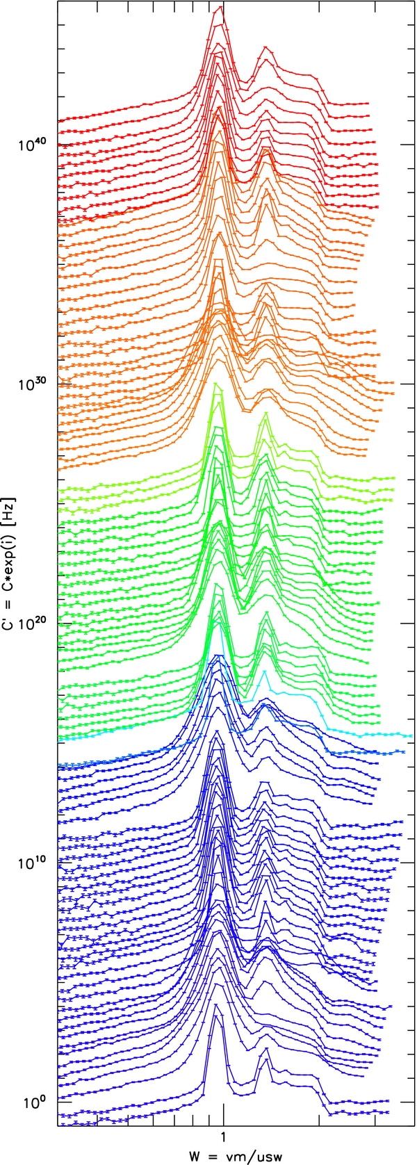
Figure 2. C' vs. W, the relative ion speed in the spacecraft frame. The spectra are stacked vertically in order of collection, the formula for which is C' = Cexp (i), where C is the true count rate and i is index number of each spectrum, which runs from 0 to 96. Note that C' is not used anywhere else in this article. Color refers to heliocentric distance: blue is ∼11 AU; greens are 16–18 AU; orange is ∼20 AU; and red is ∼21 AU.
Download figure:
Standard image High-resolution imageThe spectra in Figure 2 are dominated by the solar wind H+ peak at W ≈ 1, usually followed by solar wind He2 + at W ≈ 1.4. Sometimes there is also a peak found between W = 1.4 and 1.7, which is most likely solar wind heavy ions (e.g., O6 +). The location in W of the solar wind peaks is found theoretically by the formula  , where m and q are particle mass and charge, respectively. This is due to the fact that each of the solar wind species has roughly the same bulk speed but a different mass; thus, the peaks have different E/q. Finally, there is a sharp drop-off of the PUI distribution at W ≈ 2; however, not all spectra display the expected sharp drop-off at W = 2. In a few spectra, the drop-off is obscured by solar wind heavy ions. Others have drop-offs at what are clearly much higher speeds, and most of these are associated with extremely hot distributions. At energies higher than the drop-off, the spectra show what appears to be the beginning of the suprathermal tail. We infer this from the fact that the spectra appear to often follow a power law with various slopes. There also appears to be variation in the relative speed W at which the suprathermal distribution begins. At times there also appears to be a small peak between W = 2 and 3, which is likely due to additional solar wind heavy ions.
3. ANALYSIS
To quantitatively diagnose the PUIs, we compare the data to a model consisting of a velocity distribution function transformed into the spacecraft frame and averaged over the entrance aperture of SWAP. The velocity distribution we used for the PUIs, derived by Vasyliunas & Siscoe (1976), includes the effects of ionization, convection, and adiabatic cooling, assuming that ions are scattered instantly and isotropically in the solar wind frame
where N is the interstellar density, which we take to be 0.056 cm−3 (Gloeckler et al. 2009), β is the production ionization rate referenced at rE, which we take to be 1 AU, u is the solar wind bulk speed, λ is the ionization length scale and is related to the loss ionization rate by the relation  , where V is the interstellar neutral bulk speed, r is the distance from the Sun, θ is the polar angle from the heliospheric nose direction (i.e., the direction from which the interstellar wind blows), w equals v/u, where v is the ion speed in the solar wind frame, and Θ is the usual Heaviside theta function, which is 0 for negative arguments and 1 otherwise.
This form assumes a certain density distribution for the interstellar neutrals, that is the "cold model," such that all ions at infinity have the same speed and direction. Within that model, we also assume that the parameter μ, which represents the ratio of the outward force of radiation pressure to the inward force of gravity, equals 1, yielding straight neutral trajectories through the heliosphere. The approximation of μ = 1 allows for mathematical simplicity and is a good approximation to the values expected around solar minimum (0.7 < μ ⩽ 1; Rucinski & Bzowski 1995), as opposed to around solar maximum (1 < μ < 1.4). For μ > 1, the cold model is qualitatively different than for μ < 1, specifically it contains a singularity surface (Thomas 1978). With these assumptions, the expression for the neutral density is

This approximate form for the interstellar neutral density is quite good in the nose direction and during solar minimum, where and when our measurements were made. See Thomas (1978) for a comparison between the cold model and a more physical but also more mathematically complex model that accounts for the temperature of the interstellar neutrals at infinity, known as the hot model. Specifically, see Figure 3 for a comparison between the hot and cold models for interstellar neutral H in the interstellar nose direction.
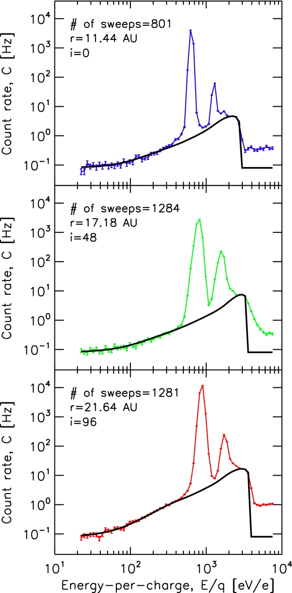
Figure 3. Coincidence count rate, C, vs. E/q spectra measured by SWAP at three distances. Thin lines connect individual data points. Error bars represent Poisson statistics. Bold lines are model comparisons (PUIs plus a background).
Download figure:
Standard image High-resolution imageThe transformation consists of two parts: a velocity shift and a conversion from distribution function to model count rate. The first, a non-relativistic velocity transformation, is v + u = vs + vm, where v is the ion velocity in the solar wind frame, u is the bulk velocity of the solar wind in the inertial frame, vs is the spacecraft velocity in the inertial frame, and vm is the ion velocity in the spacecraft frame. For this analysis, we assume that u is constant and in the radial direction.
To find v, we use the formula
where v is the magnitude of v, etc. and ⊥ and ∥ refer to perpendicular and parallel to the radial direction, respectively. Figure 1 also shows the speeds vs, ∥ and vs, ⊥. ϕ is a coordinate in the spacecraft reference frame that describes the direction from which a particle arrives. ϕ = 0 represents a particle arriving in the center of SWAP's field of view (FOV). We also assume for this analysis that ϕ = 0 corresponds to the anti-radial direction, which is not strictly true. However, it is a good approximation since theoretically the Earth–spacecraft–Sun angle is never more than 6° at these distances. Since SWAP has no directional information and a large FOV, the angle ϕ must be integrated over to find the count rate. Hence, the conversion from distribution function to count rate is
where Δϕ is the planar FOV of the instrument, 276°, vm is the E/q of the instrument converted into speed assuming protons, and g is the geometric factor of the instrument shown in Randol et al. (2012) that accounts for the increase in g with decreasing E/q due to focusing within the post-acceleration region of the instrument, normalized to the laboratory value measured at 1 keV e−1, ∼2.1 × 10⁻³ cm2 sr eV eV−1 (McComas et al. 2008a).
Three examples of the comparison between model and data are given in Figure 3. These examples display a range of different solar wind conditions. For good agreement between model and data at the lowest energies, we included a model background count rate to the model PUI distribution. This background rate was found to vary between 0.05 and 0.09 Hz, which is quite reasonable. As can be seen, the quality of the comparison is very good at low energies and near the PUI drop-off. This was done intentionally to optimize the agreement between model and data where the PUIs are most dominant. At all other energies, PUIs are overwhelmed by the larger signal of the solar wind distributions.
4. RESULTS
Figure 4 shows the ionization rate derived from the model PUI distributions versus time. The filled circles are βL, the ionization loss rate, calculated from the parameter λ such that  , where V is the interstellar neutral bulk speed, taken to be 23.2 km s−1 (McComas et al. 2012). Open circles are β as written in Equation (1). The dashed line represents the latest estimate of the total ionization rate as derived from Solar and Heliospheric Observatory Solar Wind Anisotropies data (Lallement et al. 2010), which agrees well with our average value during the same time period. The systematic increase in both ionization rates with time is consistent with the increase in solar activity since 2008.
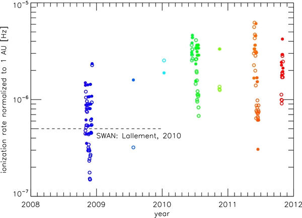
Figure 4. Ionization rates derived from model comparisons to data vs. time. Filled circles are β, the production ionization rate, and empty circles are βL, the ionization loss rate, as in Equation (1).
Download figure:
Standard image High-resolution imageFigure 5 shows β as a function of βL, with the dashed line representing β = βL. As can be seen, the two ionization rates do not match. On average, βL is a factor of ∼2 higher than β, with a standard deviation of ∼1. Roughly the same factor is found by Gloeckler et al. (1997), taking into account their different values of N and V. The derived bulk speed is shown in Figure 6.
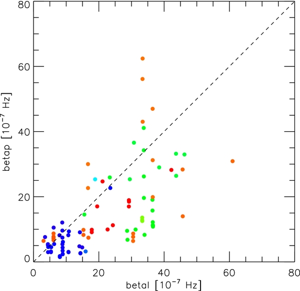
Figure 5. The ionization production rate, β, vs. the ionization loss rate, βL, found from model comparisons to SWAP data. The dashed line is β = βL.
Download figure:
Standard image High-resolution image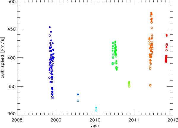
Figure 6. Model bulk speeds vs. time. Filled circles represent u, the bulk speed of the PUI distribution, and empty circles are uSW, the bulk speed of the solar wind proton distribution.
Download figure:
Standard image High-resolution imageFinally, Figure 7 shows the thermal pressure calculated from the PUI model results versus distance. Using spherical coordinates, the thermal pressure, p, is found in the usual way by performing the integral
where m is the particle mass. Substituting Equation (1) into Equation (5), the thermal pressure is
where  is the exponential integral. In Figure 7, we set θ to zero to remove the θ-dependence from the thermal pressure, so as to better show its evolution with distance. The filled circles represent each of the 97 spectra. The error bars represent the mean plus or minus one standard deviation in each distance bin (see Table 1). We bin each 1 AU beginning at 11 AU exactly, but the error bars are placed at the mean distance of the actual data in the bin to overlay the individual data points. We also show steady-state model curves, calculated from Equation (6) like the data, but instead using constant parameters. u is taken to be 440 km s−1, N and V are kept at 0.056 cm−3 and 23.2 km s−1, and the steady-state β is taken to be
  . The blue curve shows the calculation with λ = 5 AU. The less than perfect agreement between the blue curve and the data at distances larger than 12 AU is mainly due to the systematic increase in β and βL as a function of time, as shown in Figure 4. Therefore, we also show as the red curve the steady-state PUI thermal pressure with λ = 15 AU, with all the other parameters the same, which is roughly the average λ of the 21–22 AU data.

Figure 7. PUI thermal pressure, p, vs. distance, r. The filled circles are PUI thermal pressures found from Equation (6) using parameters derived by comparing the model to each individual spectrum. Error bars represent standard deviations from the mean of each distance bin. The squares are indirect PUI thermal pressure measurements from Voyager 2 (Burlaga et al. 1996). The curves labeled SW and Mag represent the solar wind thermal and magnetic pressures derived from fitting power laws to Voyager 2 measurements inside ∼40 AU (Burlaga et al. 1996). The diamonds represent several key direct measurements of PUIs from Ulysses SWICS (Gloeckler et al. 1993, 1995, 1997). The two other curves represent calculations of the PUI thermal pressure using Equation (6) and average steady-state parameters. The two colors red and blue represent different values of the ionization length scale, λ, used in the calculations, 5 and 15 AU, which are the average 11 and 21 AU values, respectively.
Download figure:
Standard image High-resolution imageTable 1. Distance Bins, Number of Events in Each, Average Distance of Events, Average PUI Thermal Pressure and Standard Deviation
| Bin | No. |  |
 |
|---|---|---|---|
| (AU) | (AU) | (10−13 dyn cm−2) | |
| 11–12 | 35 | 11.62 | 1.74 ± 1.12 |
| 12–13 | 0 | ... | ... |
| 13–14 | 1 | 13.96 | 0.52 |
| 14–15 | 0 | ... | ... |
| 15–16 | 1 | 15.53 | 3.21 |
| 16–17 | 6 | 16.95 | 2.02 ± 0.76 |
| 17–18 | 16 | 17.21 | 1.55 ± 1.02 |
| 18–19 | 3 | 18.37 | 0.95 ± 0.04 |
| 19–20 | 0 | ... | ... |
| 20–21 | 25 | 20.27 | 2.41 ± 1.45 |
| 21–22 | 10 | 21.60 | 2.00 ± 0.79 |
Download table as: ASCIITypeset image
The other points placed on the plot are from other sources from which the H+ PUI thermal pressure could be determined. To calculate the first set (diamonds), we used parameters and uncertainties derived from direct measurements of H PUIs by the Ulysses Solar Wind Ion Composition Spectrometer (SWICS; Gloeckler et al. 1993, 1995, 1997). For convenience, we list the parameters of Gloeckler et al. (1997): N = 0.115 cm−3, V = 20 km s−1, β = 2.7 × 10⁻⁷ Hz, βL = 8.5 × 10⁻⁷ Hz, r = 4.88 AU, u = 475 km s−1. The interstellar parameters at r = 2.34 AU (Gloeckler et al. 1995) and r = 4.82 AU (Gloeckler et al. 1993) are similar, except that the measurement at 2.34 AU has a bulk speed, u = 780 km s−1. If that speed is reduced to 440 km s−1, then the point nearly lies on the blue curve, as shown by the gray diamond. By contrast, the black diamond at 2.34 in the figure shows the same calculation but with u = 780 km s−1.
The second set (squares) is an indirect measurement of the PUI thermal pressure based on observations of pressure-balanced structures (PBS) by Voyager 2 at 35, 41, and 43 AU (Burlaga et al. 1996); they are necessarily indirect because the Voyager 2 instrumentation cannot measure PUIs directly. In a PBS, the PUI thermal pressure is found by assuming a pressure balance between the solar wind, magnetic field, and PUIs. Then as a change in pressure is observed in two of these three, the third can be inferred. Note that the PUI thermal pressures from the Ulysses and Voyager 2 measurements have slightly different parameters associated with them. Again, we remove any θ dependence by setting θ to 0. These points agree with the steady-state model PUI thermal pressure, with the exception of the first PBS point, as it was derived from data taken during a type of large-scale pressure enhancement known as a merged interaction region. The other model curves in the plot are the solar wind thermal and magnetic field pressure derived by fitting Voyager 2 data taken between 1978 and 1991; the equations are power laws with distance, with indices of −2.01 (Mag) and −2.85 (SW; Burlaga et al. 1996).
4.1. Correlation with Solar Wind
We also quantitatively assess the solar wind peak with a Maxwellian model velocity distribution function
where n is the local particle density, τ is the thermal width of the distribution, and v is again the ion speed in the solar wind frame, found with Equation (3), except with uSW instead of u, where uSW is the bulk speed of the solar wind. Model count rates are derived from this distribution using Equation (4), and parameters are derived by comparing the model to data.
Figure 6 shows as open circles the solar wind bulk speed, uSW. The variations in uSW are similar to those of u. Figure 8 shows u, the PUI bulk speed, versus uSW, the solar wind bulk speed, with the dashed line representing u = uSW. u generally agrees with uSW; however, on average, u is greater than uSW by ∼8 km s−1, with a standard deviation of all observations of ∼11 km s−1; the standard deviation of the mean is ∼1 km s−1. The extreme cases of extended drop-offs are obvious in Figure 8; these and more subtle cases may contribute to the difference. However, a difference has been observed elsewhere and attributed to either Alfvén wave streaming (Schwadron 1998) or to the bulk speed of the neutral distribution (Möbius et al. 1999), both of which are neglected in the derivation of Vasyliunas & Siscoe (1976) and hence our analysis also.
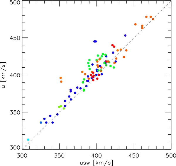
Figure 8. Model bulk speed of the PUI distribution, u, vs. model solar wind speed, uSW. The dashed line is u = uSW.
Download figure:
Standard image High-resolution imageWe also compared the variations in flux of PUIs and solar wind. First, we constructed Figure 9 so as to compare to a similar figure in Möbius et al. (2010). The plot shows the solar wind flux versus the sum of the model PUI count rate between W = 1.45 and W = 1.85, with error bars representing the Poisson statistics. The upper solid line is a power law fit to the data, and the equation of the line is in the upper left hand corner of the plot; the lower solid line is another fit with the data weighted by the uncertainties. In both cases, we find a power law dependence of PUI peak count rate on solar wind flux of ∼0.7; whereas Möbius et al. (2010) found ∼0.3 for He PUIs at 1 AU. The difference in indices could be due to the larger charge-exchange cross-section of H-H+ as compared to He-H+.
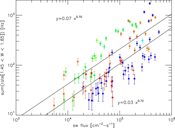
Figure 9. PUI model count rate summed over the range of W as indicated in the figure with error bars as Poisson statistics vs. solar wind flux derived from model comparisons to data. The solid lines are power law fits to the data, with (lower) and without (upper) statistical weighting. The equations of the resulting fits are shown, where the upper equation corresponds to the upper curve and the lower equation to the lower curve.
Download figure:
Standard image High-resolution imageNext, we compared solar wind flux versus the sum of the PUI differential energy flux between W = 1.6 and 2 as in Gloeckler et al. (1994) and found a high correlation (ρ ≈ 0.8), where ρ is the sample Pearson correlation coefficient, whereas Gloeckler et al. (1994) found a low correlation (ρ ≈ 0.5). One difference between those studies and ours is that we perform our sums over model curves instead of data directly in order to avoid contamination of the PUI data in that energy range by solar wind heavies. We also found a very good correlation (ρ ≈ 0.9) between solar wind flux, nuSW, and PUI flux, calculated using the equation in Vasyliunas & Siscoe (1976). Our results, along with those of Möbius et al. (2010), support the hypothesis that solar cycle phase affects the degree of correlation between solar wind and PUI fluxes (Randol & McComas 2010).
Lastly, we examine the ratio of the PUI thermal pressure to the solar wind thermal pressure. The solar wind thermal pressure, pSW, is also found using Equation (5), with a result of

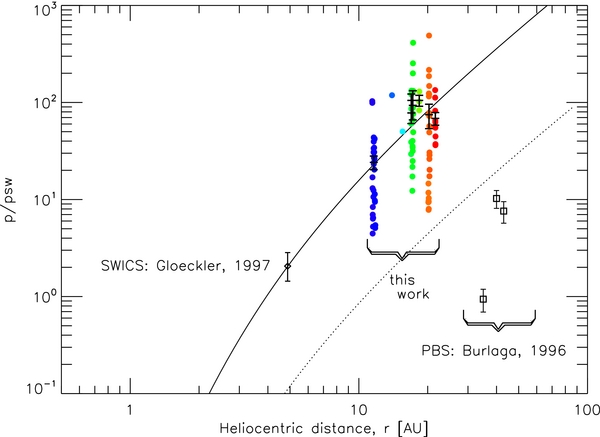
Figure 10 shows the ratio of p to pSW versus distance. Each filled circle is the ratio for each individual spectrum. The error bars represent the mean ratio in each bin plus or minus the standard deviation of the mean. The data points shown as squares are as given by Burlaga et al. (1996), again derived from PBS. We found the data point shown as a diamond by calculating the solar wind thermal pressure using Equation (8) with n and τ as given in Gloeckler et al. (1997): 0.09 cm−3 and 10.5 km s−1, respectively. The dotted line is the ratio of the PUI thermal pressure curve with λ = 5 AU from Figure 7 divided by the solar wind thermal pressure curve also from that figure. The solid line is the dotted curve normalized to the Gloeckler et al. (1997) ratio, which roughly passes through all of our data points. The measured ratio and scaled model ratio (solid line) is higher than the model ratio without scaling (dotted curve in Figure 10) due to lower solar wind thermal pressures than those from Voyager 2.
Figure 10. Ratio of PUI thermal pressure, p, to solar wind thermal pressure, pSW, vs. heliocentric distance, r. The filled circles represent the values found from each individual spectrum. The error bars represent the mean plus or minus one standard deviation of the mean in each distance bin. The diamond is p/pSW as derived from Ulysses SWICS measurements (Gloeckler et al. 1997). The squares represent the ratio of indirectly measured PUI thermal pressures and direct solar wind thermal pressures derived from Voyager 2 data (Burlaga et al. 1996). The dotted curve represents the ratio of the curves labeled λ = 5 AU and SW in Figure 7. The solid line represents the dotted line renormalized to pass through the data.
Download figure:
Standard image High-resolution image
5. DISCUSSION
The above isotropic model used to analyze the data, first formulated in Equation (11b) of Vasyliunas & Siscoe (1976), is based on ions being picked up in an azimuthal magnetic field, and our observations were taken near the ecliptic plane at large heliocentric distances, where the magnetic field is azimuthal. A PUI anisotropy is observed only in a quasi-radial field (Gloeckler et al. 1993, 1995, 1997; Oka et al. 2002; Saul et al. 2007), as predicted by theories (Isenberg 1997; Schwadron 1998; Lu & Zank 2001).
The first published SWAP PUI spectrum appeared anisotropic (McComas et al. 2010), since it had higher fluxes at low energies, which is the main signature of the PUI anisotropy (see e.g., Gloeckler et al. 1995). However, even a model spectrum with an extremely anisotropic PUI distribution underestimated the data at these lower energies. Randol et al. (2012) showed that SWAP has a geometric factor (i.e., sensitivity) that is larger at low energies than previously realized. Thus, when this geometric factor was taken into account, the need for the PUI anisotropy was eliminated. Likewise in this study of SWAP PUI data, we used the more accurate geometric factor and thus needed no PUI anisotropy.
The PUI model we used employs the cold model of the interstellar neutral density with μ, the ratio of radiation pressure to gravity, equal to 1. Although this is a good approximation for the nose direction and around solar minimum, the interstellar parameters derived from the model would be slightly different using a more realistic model for the interstellar distribution such as the "hot model" (Thomas 1978) or a more sophisticated transport model such as that found in McComas et al. (2010). Conversely, a major point of this study is how well the data is described by the classic model from Vasyliunas & Siscoe (1976). Only 5%–10% of the data were difficult to reconcile with this model due to the high speed and gradual drop-off. These could be contamination from solar wind and suprathermal tail particles, or another possibility is that the PUIs were locally heated by changes in solar wind density or magnetic field strength (Siewert & Fahr 2008).
Gloeckler et al. (1997) used the hot model of the interstellar medium to derive their parameters. Parameters derived with the cold model will be slightly different. Also, we took the Gloeckler et al. (1997) parameters and entered them into Equation (6), which is derived from the cold model, to find the thermal pressure in Figure 7. A more general expression or value for the PUI thermal pressure that is derived from the hot model would no doubt be different, a topic that could be taken up in a future study.
There is the possibility that some variation in the PUI parameters could be due to contamination from various solar wind components. While we did not attempt to account for this effect at this stage of analysis, it should be possible for at least a portion of the data, particularly when both alpha particle and heavy ion peaks are clearly visible. Another possible component is the inner source of PUIs. Randol & McComas (2010) showed that all of these components can be taken together to achieve a good fit. However, there is some doubt as to the origin of the inner source, especially of hydrogen. Randol et al. (2010) showed that the response of the instrument contains wings that may mimic the inner source in height as well as width. Resolution of this important topic should be taken up in a future study.
We infer from the data an average p/pSW ratio of the order of 1000 near the termination shock (TS), ∼80 AU, whereas Burlaga et al. (1996) predicted ∼100. The main reason our p/pSW ratio is more than a decade larger than in Burlaga et al. (1996) is that our solar wind thermal pressure is much lower than their fitted Voyager 2 thermal pressure. This decrease in solar wind thermal pressure is at least qualitatively consistent with the decrease in solar wind thermal pressure between the last two solar minima, as measured by Ulysses SWOOPS (see Figure 2 and Table 1 of McComas et al. 2008b). It should be noted that the variation in the data is large, and so a ratio of 100 is not ruled out. A recent model calculation shows a p/pSW ratio at the TS on the order of, though still smaller than, our predicted value (Zhang & Schlickeiser 2012). The effect of a higher relative pressure of PUIs at the TS would likely be a weaker shock (Zank et al. 1996; Richardson et al. 2008; Burlaga et al. 2008; Decker et al. 2008).
The fits to the Voyager 2 thermal and magnetic pressures were performed for data inside ∼40 AU. After ∼30 AU, Voyager 2 solar wind temperature measurements appear to flatten or possibly increase (Smith et al. 2001). If we had used all of the available Voyager 2 data to predict p/pSW at the termination shock, then the value would be much lower. However, this temperature flattening may be an effect of the Voyager 2 spacecraft's departure from the ecliptic plane after 30 AU (Usmanov et al. 2011; Usmanov et al. 2012). In fact, this data set can possibly be used to test the theory of Smith et al. (2001) that the solar wind in the outer heliosphere is heated in part by the dissipation of PUI-generated waves.
6. CONCLUSION
We have presented high-quality energy spectra of the interstellar pick-up ion distribution between 11 and 22 AU. Before New Horizons, few direct measurements of PUIs were made beyond 10 AU. We analyzed these spectra using a model for the PUI velocity distribution that includes convection, adiabatic cooling, ionization of neutral interstellar gas, and instantaneous and isotropic scattering in the solar wind frame (Vasyliunas & Siscoe 1976). This model has been used extensively in previous studies, and one of our main conclusions is that it works very well at these distances. We compared the ionization rate normalized at 1 AU with an independent measure of the same parameter and found good agreement.
The thermal pressure of PUIs as a function of distance based on these results tends to agree well with previous results. The calculated ratio of PUI thermal pressure to solar wind thermal pressure is considerably higher than previous results would imply; this appears to be due to lower solar wind thermal pressure during our measurements.
The PUI model results were compared with solar wind H+ model results. In general, we find a good agreement between the bulk speeds, with a PUI speed that is higher by a small but statistically significant amount. We also find that the solar wind flux is well correlated with several related measures of the PUI flux. This result is consistent with some previous results and inconsistent with others.
We thank all the members of the SWAP and New Horizons teams without whom this work would not have been possible. This work was funded as a part of the SWAP instrument work on the NASA New Horizons mission (Contract No. NASW-02008).