


ABSTRACT
We present the fundamental stellar and planetary properties of the transiting planetary system WASP-13 within the framework of the Homogeneous Study of Transiting Systems (HoSTS). HoSTS aims to derive the fundamental stellar (Teff, [Fe/H], M⋆, R⋆) and planetary (Mpl, Rpl, Teq) physical properties of known transiting planets using a consistent methodology and homogeneous high-quality data set. Four spectral analysis techniques are independently applied to a Keck+HIRES spectrum of WASP-13 considering two distinct cases: unconstrained parameters and constrained log g from transit light curves. We check the derived stellar temperature against that from a different temperature diagnostic based on an INT+IDS Hα spectrum. The four unconstrained analyses render results that are in good agreement, and provide an improvement of 50% in the precision of Teff, and of 85% in [Fe/H] with respect to the WASP-13 discovery paper. The planetary parameters are then derived via the Monte Carlo Markov Chain modeling of the radial velocity and light curves, in iteration with stellar evolutionary models to derive realistic uncertainties. WASP-13 (1.187 ± 0.065 M☉; 1.574 ± 0.048 R☉) hosts a Saturn-mass, transiting planet (0.500 ± 0.037 MJup; 1.407 ± 0.052 RJup), and is at the end of its main-sequence lifetime (4–5.5 Gyr). Our analysis of WASP-13 showcases that both a detailed stellar characterization and transit modeling are necessary to well determine the fundamental properties of planetary systems, which are paramount in identifying and determining empirical relationships between transiting planets and their hosts.
Export citation and abstract BibTeX RIS
1. INTRODUCTION
The detection and characterization of a large number of extrasolar planets with a variety of physical properties, in different environments and with a range of ages, is necessary for the understanding of the formation and evolution of planetary systems. It is only with precise measurements of the fundamental properties of the exoplanets and their host stars that the planetary bulk composition can be inferred and the planetary structure probed, and thus, we can explore the underlying physical processes involved in their formation and evolution.
Transit surveys, such as SuperWASP (Pollacco et al. 2006), have been extremely successful in discovering planets for which measurements of their masses and radii are possible. These have revealed a large diversity of physical properties of the extrasolar planets and their host stars (see, e.g., Baraffe et al. 2010). With more than 290 transiting exoplanets confirmed to date,14 it is now possible to conduct statistical studies of planetary properties, and thus, derive more robust empirical relationships between the planets and their host stars. For example, it is generally thought that in the case of hot Jupiters the planetary radius is correlated with the planet equilibrium temperature and the stellar irradiation, and anticorrelated with stellar metallicity (e.g., Santos et al. 2004; Guillot et al. 2006; Laughlin et al. 2011; Enoch et al. 2012; Faedi et al. 2011; Demory & Seager 2011). Buchhave et al. (2012), using recent Kepler results, find that giant planets are found around metal-rich stars, while those with radii smaller than four times that of the Earth are found to orbit stars with a large range in metallicity (−0.6 ⩽ [Fe/H] ⩽ 0.5 dex). This is compatible with previous observational results (Udry & Santos 2007; Sousa et al. 2008, 2011a; Ghezzi et al. 2010), which show that Neptunian planets do not form preferentially around metal-rich stars. Moreover, Adibekyan et al. (2012a, 2012b) show that although the terrestrial planets can be found in a low-iron regime, they are mostly enhanced by alpha elements as compared to stars without detected planets showing that metals continue to be important also for the formation of these planets.
This paper presents the pilot study of our project, entitled Homogeneous Study of Transiting Systems (HoSTS), that will derive a homogeneous set of physical properties for all transiting planets and their host stars, aiming to minimize the effects of any systematics in the measurements due to the quality of the data and/or technique applied. Individual studies of single planetary systems make systematic uncertainties difficult to identify, and quantify. For example, Mancini et al. (2012) found HAT-P-8b to have a radius ∼14% smaller than previous estimates (a difference larger than the quoted uncertainties), making it consistent with other transiting planet radii, and not significantly inflated. As more planets are being discovered and/or re-analyzed, the observed trends, like the anomalously large planetary radii, remain to be confirmed. A number of recent studies employing consistent analysis procedures for subsets of the known stars with transiting planets have been attempted (e.g., Torres et al. 2008; Ammler-von Eiff et al. 2009; Southworth 2008, 2009, 2010, 2011, 2012); however, these have largely employed heterogeneous spectroscopic data sets and adopted the stellar properties, like Teff and [Fe/H], from the literature. Because these measurements are non-homogeneous—arising from different spectroscopic analysis techniques applied to spectra obtained with different spectrographs, different resolution, etc.—the typically quoted uncertainties of ∼10% in the published stellar and planetary mass and radius likely contain currently uncharacterized systematics. More recently, Torres et al. (2012) have thoroughly analyzed new and archival spectra (from different instruments, and with varied signal-to-noise ratio and resolution) of 56 transiting planet hosts comparing three different stellar characterization methods. Torres et al. (2012) focused on the stellar hosts, deriving a new set of homogeneous spectroscopic stellar properties and have been able to identify systematic errors due to the stellar characterization techniques applied. Thus, any empirical trend identified among the physical properties, like the observed inflated radii of hot Jupiters with respect to planetary models, may have to be revised.
HoSTS extends these previous studies in that the stellar host properties are derived from a homogeneous, high-quality spectral data set applying four stellar characterization techniques, and that the planetary properties are also derived consistently. By means of our homogeneous spectral data set and subsequent analyses, we will be able to investigate systematic uncertainties on the derived stellar properties arising not only from the methodology, as exemplified by Torres et al. (2012), but also from the quality of the data. We will combine iteratively our results with the best available radial velocity data and transit photometry in the literature to derive a homogeneous set of properties for the transiting systems. The resulting consistent set of physical properties will allow us to further explore known correlations, e.g., core size of the planet and stellar metallicity, and to newly identify subtle relationships providing insight into our fundamental understanding of planetary formation, structure, and evolution. And thus, this will allow us to reevaluate the planetary properties, of each planet alone, and with respect to different planet populations.
In this paper, we present our HoSTS pilot study of the transiting system WASP-13 which is composed of a Saturn-mass planet around an early G-type star. Section 2 describes both the data acquired by our team and the data from the literature utilized in our analyses. Section 3 describes the spectral analysis of the WASP-13 spectra implementing four different techniques in order to derive the stellar spectroscopic properties. For each of the four stellar characterization methods, we present two different cases for which stellar properties have been derived: (1) an unconstrained analysis where all parameters are left free and (2) applying an external constraint on log g. We have used the temperature diagnostic based on Hα to verify the values derived from the stellar characterization methods, as well as the effect of fixing Teff on the other spectroscopically determined stellar properties. Then we describe the modeling of the system's radial velocity and light curves to derive the stellar and planetary properties. In Section 4, we discuss the results from our pilot study of WASP-13, and outline the future work of the HoSTS project.
2. DATA
For our analysis of the planetary system WASP-13, we have acquired new spectroscopic data described below in Sections 2.1 and 2.2, and have utilized the data available from the literature and the SuperWASP archive. The SuperWASP light curve includes over 12,100 data points observed with the SuperWASP-North facility in La Palma, Spain (Pollacco et al. 2006) from 2006 November to 2009 April (see Figure 1, left panel). These data expand the span of the SuperWASP light curve from that of the discovery paper for two additional years, and have a median photometric uncertainty of 0.006 mag. From Skillen et al. (2009), we have obtained the system's radial velocities acquired with the SOPHIE instrument mounted on the 1.9 m telescope at the Haute Provence Observatory (see Figure 1, right panel), as well as the James Gregory Telescope (JGT) differential photometry in the R band. Additionally, we have adopted the high-cadence, high-precision light curves observed with the RISE instrument on the Liverpool Telescope published by Barros et al. (2012). All follow-up light curves are shown in Figure 2.
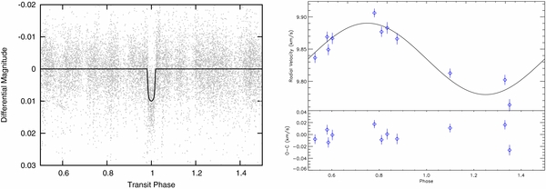
Figure 1. Left: SuperWASP-N light curve of transiting planetary system WASP-13. Comprising over 12,100 data points and spanning from 2006 November to 2009 April, the SuperWASP light curve is shown with gray points with the model transit light curve (see Section 3.3) in black. The photometric data have been folded over the orbital period and exhibit at phase zero the characteristic dip in brightness as the Saturn-mass planet WASP-13b (Mpl = 0.50 ± 0.01 MJup) passes in front of its host star, blocking part of the stellar light every 4.353 days. The median photometric uncertainty of the light curve is 0.006 mag. Right: the radial velocity measurements from the SOPHIE instrument at the Observatoire d'Haute Provence (Skillen et al. 2009) are shown against the our model radial velocity curve that describes the reflex motion of WASP-13 due to the presence of the planet. The residuals to the fit are shown in the lower panel.
Download figure:
Standard image High-resolution image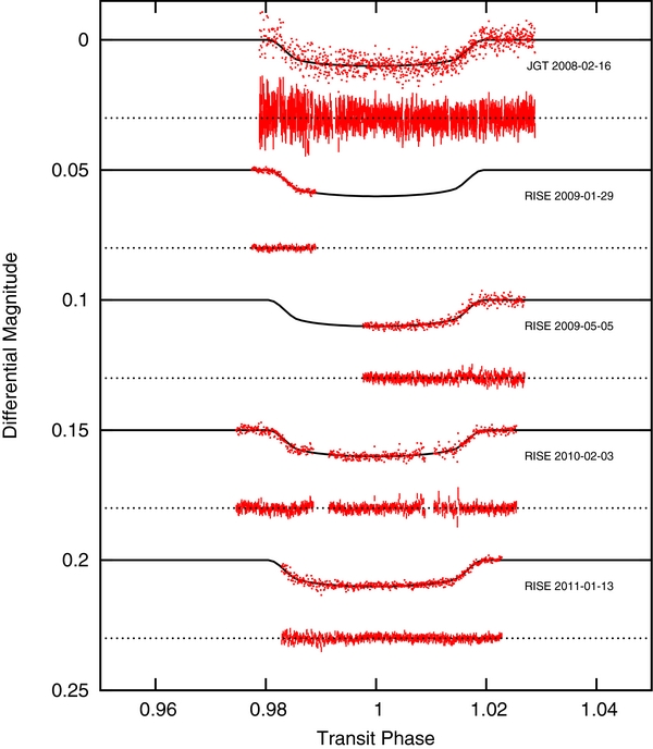
Figure 2. WASP-13b follow-up transit light curves. The transit light curves of the WASP-13 system from JGT (Skillen et al. 2009) and RISE (Barros et al. 2012) are shown in red points overplotted with the model light curves (in solid black lines) from our MCMC analysis (Section 3.3), with their corresponding residuals including the uncertainty of the photometric data directly below (red error bars). The light curves and residuals have been shifted vertically from zero for clarity.
Download figure:
Standard image High-resolution image2.1. WASP-13 Hα Long-slit Spectrum
For this work, we obtained a long-slit spectrum of the planet host WASP-13 around the Hα line using the Intermediate Dispersion Spectrograph (IDS) mounted on the 2.5 m Isaac Newton Telescope at the Roque de los Muchachos Observatory in La Palma, Spain. We used the H1800V grating with the RED+2 CCD, and a 1 4 slit yielding a dispersion of 0.35 Å pixel−1 and a resolution of R ∼ 10,000 at 6560 Å. The observations of WASP-13 and the standard calibrations, including a spectrum of Vega and Arcturus, were taken on 2012 May 8 and 9. To allow for a precise measurement of the Hα profile, the WASP-13 spectrum had a signal-to-noise ratio of ∼500 as calculated by the IDL function DER_SNR. The derived temperature (Section 3.1) is used as an independent check on the effective temperature of WASP-13 derived from the stellar characterization methods.
2.2. WASP-13 HIRES Spectrum
We observed WASP-13 on 2011 March 14 UT with the High Resolution Echelle Spectrograph (HIRES) on Keck-I (Vogt et al. 1994). We observed in the spectrograph's "red" (HIRESr) configuration with an echelle angle of −0 018 and a cross-disperser angle of 0737. We used the KV418 order-blocking filter and the 057 × 70 slit, and the chip was binned by 2 pixels in the spatial direction during readout. The resulting resolving power is R ∼ 72,000.
We obtained three consecutive integrations of WASP-13, each of 600 s. ThAr arc lamp calibration exposures were obtained before and after the WASP-13 exposures, and sequences of bias and dome flat-field exposures were obtained at the end of the night. The WASP-13 exposures were processed along with these calibrations using standard IRAF15 tasks and the MAKEE reduction package written for HIRES by T. Barlow. The latter includes optimal extraction of the orders as well as subtraction of the adjacent sky background. The three exposures of WASP-13 were processed separately and then median combined with cosmic-ray rejection into a single final spectrum. The signal-to-noise ratio of the final spectrum is ∼300 per resolution element.
3. ANALYSIS
In this section, we describe the methods applied to our WASP-13 data set in order to derive the physical properties of the planetary system.
3.1. Determination of Teff from Hα Spectrum
This analysis is based on the Hα spectrum of WASP-13 described in Section 2.1. The Balmer lines provide an excellent Teff diagnostic for stars cooler than about 8000 K due to their virtually nil gravity dependence (Gray 2008). Normalization of the observations is critical, which the shape of the Balmer line must be preserved (Smith & Dworetsky 1988). The extracted spectrum was normalized using a low-order polynomial fitted to the continuum regions more than 100 Å either side of Hα, in order to avoid any distortion due to the weak wings of this profile. The spectrum was then analyzed using uclsyn with Castelli et al. (1997) ATLAS9 models with no overshooting and Hα profiles calculated using VCS theory (Vidal et al. 1973). The best-fitting Hα profile has Teff = 5850 ± 60 K.
However, the use of Balmer lines as temperature diagnostics is not without its difficulties due to uncertainties caused by different line broadening theories (Stehlé & Hutcheon 1999; Barklem et al. 2000; Allard et al. 2008), the treatment of atmospheric convection (Gardiner et al. 1999; Heiter et al. 2002), and non-local thermodynamic equilibrium (LTE) effects (Barklem 2007). We, therefore, also fitted the Hα profile in the KPNO solar spectrum (Kurucz et al. 1984) which gave a Teff 70 ± 20 K lower than the direct value of 5777 K. Thus, Hα appears to underestimate stellar effective temperatures. Adding 70 ± 20 K to the Teff derived above, it gives Teff = 5920 ± 60 K for WASP-13. This was recently investigated in detail by Cayrel et al. (2011) who found similar systematic differences, and provide a correction:

with an uncertainty of 31 K. Applying this correction, and adding the errors in quadrature, gives Teff = 5950 ± 70 K for WASP-13.
Both temperatures from our Hα temperature diagnostic agree with each other, and with the Teff derived from the infrared flux method (Teff = 5935 ± 183 K; Skillen et al. 2009). Moreover, they are consistent with the temperatures derived in the stellar characterization methods described below.
3.2. Stellar Characterization Analysis
We apply to the HIRES echelle spectrum (Section 2.2) four different stellar characterization methods that are extensively used in the exoplanet literature. Each method is done independently from each other and is described in the subsections below (Sections 3.2.1–3.2.4). Method A is based on the technique of spectral synthesis, which compares an observed spectrum to synthetic model spectra generated for a range of stellar parameters. The best-fitting model (based on a χ2 minimization) defines the final atmospheric parameters. The other three methods (B, C, and D) are based on the principle of excitation/ionization equilibrium of iron lines, in which equivalent width (EW) measurements of many lines are used to determine iron abundance, and the stellar atmospheric properties. Methods B, C, and D are each unique in their choice of line lists, model atmospheres, EW measurements, continuum normalization, and convergence criteria. Furthermore, Method B makes an absolute iron abundance measurement of the star, whereas the other three methods are differential analyses, and derive a stellar metallicity relative to the Sun. Method A includes a careful determination of the line list parameters, i.e., excitation potential and oscillator strength, to match the spectrum of the Sun using spectral synthesis. Method C does a differential line-by-line analysis relative to the Sun using the same instrument setup, whereas Method D uses measured EWs and a standard solar iron abundance (e.g., 7.50 ± 0.04; Asplund et al. 2009) to derive the line properties.
For each of the four stellar characterization methods, we present two distinct cases: (1) the unconstrained analysis, where Teff, log g, and [Fe/H] (and vsin i when appropriate) are derived freely; and (2) constraining log g from the mean stellar density as determined from the transit model to derive the other stellar properties. The spectroscopically determined stellar parameters derived for each case above with all four methods are shown in Table 1. Furthermore, the Teff derived using a different temperature diagnostic based on an Hα spectrum is used to check the stellar properties in Table 1, as well as to explore the effect on the derived stellar spectroscopic properties by fixing Teff. The resulting spectroscopic properties are shown in Table 2.
Table 1. Spectroscopically Determined Stellar Parameters of WASP-13
| A | B | C | D | Weighted Meana | |
|---|---|---|---|---|---|
| Unconstrained | |||||
| Teff (K) | 6003 ± 65 | 5955 ± 75 | 5919 ± 30 | 6025 ± 21 | 5989 ± 16 ± 48 |
| log g | 4.16 ± 0.08 | 4.13 ± 0.11 | 4.02 ± 0.06 | 4.19 ± 0.03 | 4.16 ± 0.03 ± 0.07 |
| log A(Fe) | 7.54 ± 0.06b | 7.60 ± 0.09 | 7.54 ± 0.05b | 7.58 ± 0.05b | 7.56 ± 0.03 ± 0.03 |
| [Fe/H] | 0.04 ± 0.05 | 0.10 ± 0.09b | 0.04 ± 0.02 | 0.08 ± 0.02 | 0.06 ± 0.01 ± 0.03 |
| vsin i (km s−1) | 5.79 ± 0.08 | 5.26 ± 0.25 | ⋅⋅⋅ | ⋅⋅⋅ | 5.74 ± 0.08 ± 0.38 |
| vt (km s−1) | 1.01 ± 0.17c | 0.95 ± 0.10 | 1.53 ± 0.09 | 1.28 ± 0.10 | 1.27 ± 0.06 ± 0.29 |
| Fixing log g = 4.10 ± 0.04 dex | |||||
| Teff (K) | 5994 ± 150 | 5955 ± 70 | 5912 ± 30 | 6048 ± 63 | |
| log A(Fe) | 7.55 ± 0.12b | 7.59 ± 0.09 | 7.54 ± 0.05b | 7.56 ± 0.07b | |
| [Fe/H] | 0.05 ± 0.11 | 0.09 ± 0.09b | 0.04 ± 0.02 | 0.06 ± 0.06 | |
| vsin i (km s−1) | 5.86 ± 0.22 | 5.26 ± 0.25 | ⋅⋅⋅ | ⋅⋅⋅ | |
| vt (km s−1) | 1.01 ± 0.17c | 1.00 ± 0.10 | 1.53 ± 0.09 | 1.33 ± 0.10 | |
Notes. aThe first error (σw) is derived from the uncertainties in the individual measurements (σi), σw = [∑1/σi]−1/2, and the second error is calculated from the standard deviation of the individual measurements. bDerived using the most current value for the solar abundance of iron, log A(Fe)☉ = 7.50 ± 0.04 (Asplund et al. 2009). cThe vt has been adopted from the empirical relationship described in Section 3.2.1, and is not included in the weighted mean.
Download table as: ASCIITypeset image
Table 2. Stellar Properties of WASP-13: Fixing Teff = 5950 ± 70 K
| A | B | C | D | |
|---|---|---|---|---|
| log g | 4.14 ± 0.19 | 4.13 ± 0.11 | 4.07 ± 0.13 | 4.06 ± 0.10 |
| log A(Fe) | 7.56 ± 0.07a | 7.60 ± 0.09 | 7.56 ± 0.06a | 7.52 ± 0.07a |
| [Fe/H] | 0.06 ± 0.06 | 0.10 ± 0.09a | 0.06 ± 0.04 | 0.02 ± 0.06 |
| vsin i (km s−1) | 5.88 ± 0.05 | 5.26 ± 0.25 | ⋅⋅⋅ | ⋅⋅⋅ |
| vt (km s−1) | 1.01 ± 0.17 | 0.95 ± 0.10 | 1.53 ± 0.08 | 1.30 ± 0.10 |
Note. aDerived using the most current value for the solar abundance of iron, log A(Fe)☉ = 7.50 ± 0.04 (Asplund et al. 2009).
Download table as: ASCIITypeset image
Given the quality of our data, and the nuances of each of the stellar characterization methods, the preferred solution for each of the four methods is that derived through the unconstrained analysis. In the last column of Table 1, we present the weighted mean of the four unconstrained solutions for each method which are used to derive the stellar mass and radius, and the planetary properties (see Section 3.3). Additionally, we report two errors on the stellar properties of Table 1: the first is calculated from the weighted quadrature sum of the individual internal errors, and the second is a measure of the systematic uncertainty based on standard deviation of the individual measurements. The systematic uncertainty is likely to be underestimated in the case of WASP-13 because only the four measurements from the unconstrained cases are taken into account. A more realistic systematic uncertainty will be possible once a larger HoSTS sample has been analyzed in the same consistent manner as we present in this paper.
3.2.1. Method A: SME
Method A consists on the implementation of Spectroscopy Made Easy (SME ver. 3.54; Valenti & Piskunov 1996) to derive stellar parameters of WASP-13 described below. We base the general method of our SME analysis on that given in Valenti & Fischer (2005) including the grid of model atmospheres and derivation of macroturbulence; however, we use a line list, synthesized wavelength ranges, and abundance pattern adapted from Stempels et al. (2007) and Hebb et al. (2009).
In general, SME uses the Levenberg–Marquardt (LM) algorithm to solve the nonlinear least-squares problem of fitting an observed spectrum with a synthetic spectrum. Like any nonlinear least-squares algorithm, the LM-based solver in SME requires a good initial guess and a smoothly varying χ2 surface in order to consistently find the absolute global minimum (what we are calling the optimal solution). In addition, a single SME best-fit solution does not allow for an estimation of the error in the solution apart from the error calculated from that solution's covariance matrix. This does not take into account the deviations from the best-fit solution depending on the specific choice of initial parameter values nor the internal precision of the solver.
We have expanded on the technique outlined in Valenti & Fischer (2005) that allows us to operate SME in an automated fashion and explore the effect of the initial conditions on the final resulting stellar parameters. Using the ACCRE High-Performance Computing Center at Vanderbilt University, we have developed an extensive Monte Carlo approach to using SME. We start by randomly selecting 500 initial parameter values from a multivariate normal distribution with five parameters: Teff, log g, [Fe/H], [M/H], and vsin i. For WASP-13, we defined this distribution using the derived stellar parameters and uncertainties from Skillen et al. (2009). The microturbulence (vt) for each of these initial values in this multivariate distribution was fixed at 1.01 ± 0.17 km s−1, estimated using a polynomial fit (Equation (1)) to the HARPS sample of stellar Teff and microturbulence (Sousa et al. 2011a) at Teff from Skillen et al. (2009). The value of vt is kept fixed throughout our SME analysis because the scatter of the HARPS sample around this temperature is larger than the change in vt in the range of temperatures explored in all cases. Furthermore, the change in the microturbulence value within its uncertainties does not affect significantly the derived [Fe/H]:

We then allow SME to find a best-fit synthetic spectrum and solve for the free parameters for the full distribution of initial guesses, producing 500 best-fit solutions for the stellar parameters. We determine our final measured stellar properties by identifying the output parameters that give the optimal SME solution (i.e., the solution with the lowest χ2). The overall SME measurement uncertainties in the final parameters are calculated by adding in quadrature: (1) the internal error determined from the 68.3% confidence region in the χ2 map and (2) the median absolute deviation of the parameters from the 500 output SME solutions to account for the correlation between the initial guess and the final fit.
Following this procedure, we solved for the parameters of WASP-13 first letting all fitted parameters be free; then using a constraint on log g, and letting the other parameters free; and finally analyzing the spectrum fixing Teff. The resulting optimal parameters and uncertainties are given in the first results column of Tables 1 and 2.
Our choice of the unconstrained analysis as the preferred solution for Method A does not follow the conclusions of Torres et al. (2012), where they suggest that fixing the log g (case b above) is the best approach when using synthesis-based methods. However, we find that our method A differs in their implementation of SME in the treatment of microturbulence, the line list, the sampling of a large parameter space in initial parameters, and the convergence criteria. Specifically our linelist includes the Na I D region between 5849--5950 Å, a gravity and temperature sensitive line, as well as the gravity sensitive Mg b triplet region. In similarity to the analyses by Torres et al. (2012) and Valenti & Fischer (2005), we did not include the Hα region due to the difficulty in normalizing the continuum for such a broad line in an echelle spectrum. A more in-depth comparison will be possible on the larger HoSTS sample, with which we will be able to state more robustly whether we need to constrain log g or not, as well as to explore the dependence of physical properties on the data.
3.2.2. Method B: UCLSYN
Method B consists in the analysis performed with the spectral synthesis package uclsyn (University College London SYNthesis; Smith & Dworetsky 1988; Smith 1992; Smalley et al. 2001) using the methods given in Doyle et al. (2013). In general, the surface gravity (log g) was determined using the ionization balance of the Fe i and Fe ii lines, as well as from the Ca i line at 6439 Å and the Na i D lines. The excitation balance of the Fe i lines was used to determine the effective temperature (Teff). A null dependence was required between Fe abundance and EW in order to ascertain the microturbulence (vt) using the Magain (1984) method. The Fe abundance was determined from EW measurements of several unblended lines, and additional least-squares fitting of lines was performed when required. The projected stellar rotation velocity (vsin i) was determined by fitting the profiles of several unblended Fe i lines. A value for macroturbulence (vmac) of 3.0 ± 0.3 km s−1 was assumed, based on the calibration by Bruntt et al. (2010).
The parameters obtained from the analysis are listed in the second column of Tables 1 and 2.
3.2.3. Method C: ARES/MOOG + Schuler Line List
In the case of the Method C for the unconstrained analysis, the atmospheric parameters (Teff, log g, and vt) and metallicity ([Fe/H]16) of WASP-13 were derived using the standard spectroscopic method based on the excitation and ionization equilibrium of Fe i and Fe ii lines. The [Fe/H] abundances were normalized on a line-by-line basis to the solar values taken from Schuler et al. (2011a). The analysis was done in LTE using the 2010 version of MOOG17 (Sneden 1973) and one-dimensional plane-parallel model atmospheres interpolated from the OVER grid of ATLAS9 models (Castelli & Kurucz 2004).
The line list was adopted from Schuler et al. (2011b) and the EWs were measured using the automatic code ARES (Sousa et al. 2007). Effective temperatures and microturbulence velocities were iterated until the slopes of [Fe/H] versus χ (the excitation potential of the lines) and log (EW/λ) (their reduced EWs) were respectively zero; i.e., until the individual [Fe/H] abundances were independent of excitation potential and reduced EWs. Surface gravities were iterated until the [Fe/H] abundances determined from Fe i and Fe ii lines were equal. The iteration of the atmospheric parameters was done automatically, using codes adapted from Ghezzi et al. (2010). Any lines with [Fe/H] abundances that deviated more than 2σ from the average were removed and the above iteration was repeated until convergence was achieved. The final line list contained 45 Fe i and 5 Fe ii lines.
The internal uncertainties on the atmospheric parameters were estimated as follows. The error of the microturbulence was determined by varying this parameter until the slope of [Fe/H] versus log (EW/λ) was equal to its standard deviation. The uncertainty of the effective temperature was obtained by changing this parameter until the slope of [Fe/H] versus χ was equal to its standard deviation. The error of vt was also taken into account when calculating the uncertainty of Teff. The error of the surface gravity was obtained by varying this parameter until the difference between the average [Fe i/H] and [Fe ii/H] abundances were equal to the standard deviation of the latter (divided by the square root of the number of Fe ii lines). The contribution from Teff was also included. Finally, the uncertainty of [Fe/H] is a combination of the standard deviation of the [Fe i/H] abundance (divided by the square root of the number of Fe i lines) and the variations caused by the errors in Teff, log g, and vt, all added in quadrature. We note that these are the internal errors of the spectroscopic differential analysis used here and that the real uncertainties (e.g., from the comparison with other similar studies) might be larger.
In the second case, the surface gravity is fixed to the value determined from the analysis of the mean stellar density (log g = 4.10 ± 0.04), the other parameters are iterated upon (with the same line list as above). The uncertainties of Teff and vt were estimated as described above. The error of the metallicity took into account all four contributions described above, but the influence of the surface gravity was estimated by varying log g by ±1σ (i.e., fixing this parameter at the values 4.06 and 4.14) and iterating the atmospheric parameters again. The larger difference between the new value and the one obtained with log g = 4.10 was taken as the error on [Fe/H] due to the uncertainty on the surface gravity. We have observed that this variation of log g has no effect on [Fe/H].
In the third case, we fixed the effective temperature to the value determined from the analysis of the Hα line (Teff = 5950 ± 70 K), and iterated the other parameters (with the same line list as above). The uncertainty of vt was estimated as in the original procedure (with free parameters). The influence of the effective temperature on the errors of the surface gravity and metallicity was determined by varying Teff by ±1σ (i.e., fixing this parameter at the values 5880 and 6020 K) and iterating the atmospheric parameters again. The larger differences between the new values and the ones obtained with Teff = 5950 K were taken as the errors on [Fe/H] and log g due to the uncertainty on the effective temperature and then added in quadrature to the other contributions, giving the final values quoted above.
3.2.4. Method D: MOOG/ARES + Sousa Line List
In the case of Method D, the spectroscopic parameters were derived starting with the automatic measurement of EWs of Fe i and Fe ii lines with ARES (Sousa et al. 2007) and then imposing excitation and ionization equilibrium using a spectroscopic analysis in LTE with the help of the code MOOG (Sneden 1973) and a GRID of Kurucz Atlas 9 plane-parallel model atmospheres (Kurucz 1993).
The Fe i and Fe ii line list is composed of more than 300 lines that were individually tested in high-resolution spectra to check its stability to an automatic measurement with ARES (Sousa et al. 2008). The atomic data of the lines were obtained from the Vienna Atomic Line Database (Kupka et al. 1999) but the oscillator strength (log gf) of the lines were recomputed through an inverse analysis of the solar spectrum allowing this way to perform a differential analysis relatively to the Sun. A full description of the method can be found in Santos et al. (2004) and Sousa et al. (2008).
We have only reported in Tables 1 and 2 the internal errors derived from our method. Typically, we report a more realistic uncertainty that considers the typical dispersion plotted in each comparison of parameters, as presented in Sousa et al. (2008). A more complete discussion about the systematic errors generally derived for this spectroscopic method can be found in Sousa et al. (2011b). However, given that in this paper we derive the systematic uncertainty from the comparison against the resulting spectroscopically determined parameters from Methods A, B, and C, we only report the internal errors for each of the three cases.
For the constrained cases, the same method was used but fixing each specific parameter (log g and Teff) in the process. We also used the same procedure for the determination of the errors for which the uncertainty in each constrained parameter was considered.
3.3. Transit Model
The planetary properties were determined using a simultaneous Markov Chain Monte Carlo (MCMC) analysis including the WASP photometry, and the high-precision photometry, together with the radial velocity measurements. A detailed description of the method is given in Collier Cameron et al. (2007) and Pollacco et al. (2008).
Our iterative fitting method uses the following parameters: the epoch of mid-transit T0, the orbital period P, the fractional change of flux proportional to the ratio of stellar to planet surface areas  , the transit duration T14, the impact parameter b, the radial velocity semi-amplitude K1, the stellar effective temperature Teff and metallicity [Fe/H], the Lagrangian elements
  and
and  (where e is the eccentricity and ω is the longitude of periastron), and the systematic offset velocity γ. The spectroscopically determined Teff and [Fe/H] presented in the last column of Table 1 with the two reported errors added in quadratures are used within our MCMC code as priors in the stellar mass determination from the empirical Torres/Enoch relationship (see below). The sum of the χ2 for all input data curves with respect to the models was used as the goodness-of-fit statistics.
An initial MCMC solution with eccentricity as a free parameter was explored for WASP-13 deriving a small eccentricity (e = 0.10). However, the probability that it is a spurious non-circular orbit as defined by Lucy & Sweeney (1971) is 1.0 in agreement with previous circular solutions for the system (Skillen et al. 2009; Barros et al. 2012). Thus, we adopt a circular orbit for the rest of our analysis. For the treatment of the stellar limb-darkening, the four-coefficient law of Claret (2000, 2004) was used with their derived coefficients in the R band for both the JGT and as an approximation for the WASP photometry, which is in a V+R passband. In the case of the RISE photometry, we used the same limb-darkening law, using the coefficients derived specifically for the RISE passband and CCD response by I. Howarth, following the procedure in Howarth (2011).
From the parameters mentioned above, we calculate the mass M, radius R, density ρ, and surface gravity log g of the star (which we denote with subscript ⋆) and the planet (which we denote with subscript pl), as well as the equilibrium temperature of the planet assuming it to be a blackbody (Tpl, A = 0) and that energy is efficiently redistributed from the planet's day side to its night side. We also calculate the transit ingress(egress) times T12(T34), and the orbital semi-major axis a. These calculated values and their 1σ uncertainties from our MCMC analysis are presented in Table 3. The observed light curves are plotted against the model light curves with their residuals in Figure 2.
Table 3. System Parameters and 1σ Error Limits Derived from the MCMC Analysis
| Parameter | Symbol | Value | Units |
|---|---|---|---|
| Transit epoch | T0 | 5305.62823 ± 0.00025 | daysa |
| Orbital period | P | 4.3530135 ± 0.0000027 | days |
| Planet/star area ratio |  |
0.00844 ± 0.00016 | |
| Transit duration | tT | 0.1668 ± 0.0010 | days |
| Impact parameter | b | 0.603 ± 0.025 | R⋆ |
| Stellar reflex velocity | K1 | 0.0555 ± 0.0036 | km s−1 |
| Center-of-mass velocity | γ | 9.8348 ± 0.0009 | km s−1 |
| Orbital eccentricity | e | 0. | fixed |
| Orbital inclination | i | 85.43 ± 0.29 | deg |
| Stellar density | ρ⋆ | 0.306 ± 0.020 | ρ☉ |
| Stellar mass | M⋆ | 1.187 ± 0.065 | M☉ |
| Stellar radius | R⋆ | 1.574 ± 0.048 | R☉ |
| Orbital semi-major axis | a | 0.0552 ± 0.0010 | AU |
| Planet radius | Rpl | 1.407 ± 0.052 | RJup |
| Planet mass | Mpl | 0.500 ± 0.037 | MJup |
| Planet surface gravity | log gp | 2.764 ± 0.038 | (cgs) |
| Planet density | ρpl | 0.180 ± 0.020 | ρJ |
| Planet temperature | Teq | 1548 ± 22 | K |
Note. aGiven in BJDTDB − 2,450,000 as defined by Eastman et al. (2010).
Download table as: ASCIITypeset image
The stellar mass of planet host star has been derived within our MCMC analysis from the empirical (Torres et al. 2010) calibration, which is based on the precisely measured masses and radii of eclipsing binary stars, and relates log g, [Fe/H], and Teff to the stellar mass and radius. However, while Teff can be determined with high precision from the stellar spectrum (see Sections 3.1 and 3.2), log g is usually poorly constrained, and thus stellar masses derived from the spectroscopic log g can have large uncertainties and can suffer from systematics. Thus, our MCMC method derives the stellar mass using the empirical calibration as described by Enoch et al. (2010), which is based on that by Torres et al. (2010) but relies on the directly measured ρ⋆, instead of log g. The stellar density, ρ⋆, is directly determined from transit light curves and as such is independent of the stellar mass, and the effective temperature determined from the spectrum (Sozzetti et al. 2007; Hebb et al. 2009), as well as of theoretical stellar models ( is assumed; see Seager & Mallén-Ornelas 2003). The error on the stellar mass that we first derived from the MCMC, which is based on the empirical relationship, seemed underestimated (∼1%), and thus so are the errors of the other properties that depend on the stellar mass (e.g., orbital separation). Therefore, we adopt a more realistic uncertainty in the stellar mass from the comparison of stellar evolutionary models to the observed properties of WASP-13, as described in the paragraph below and is shown in Figure 3. This uncertainty in the stellar mass is included in the final MCMC analysis (see Table 3) and is propagated through all other dependent parameters.
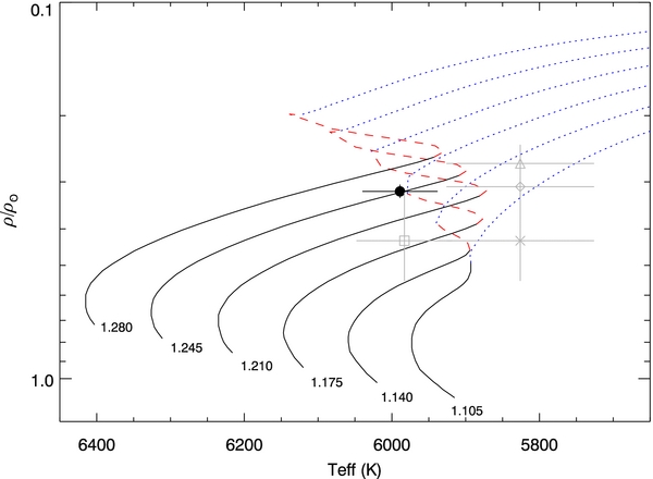
Figure 3. Parameters of WASP-13 compared to the Y2 stellar evolution models (Demarque et al. 2004). The effective temperature and mean stellar density of WASP-13 is plotted as a solid circle. The six mass tracks have been interpolated in metallicity to [Fe/H] = +0.06 to match the measured value of WASP-13. The mass of each track is labeled at the bottom of each line. Different evolutionary phases—main-sequence evolution (solid black), overall contraction phase (dashed red), and post-main sequence (blue dotted)—are given different line styles. Previous measurements of WASP-13 are also plotted in gray—diamond (Barros et al. 2012), triangle (Southworth 2012), square (Torres et al. 2012), and asterisk (Skillen et al. 2009). The best mass for WASP-13 derived from these tracks is 1.245 M☉ if the star is on the main sequence, but a 1.175 M☉ star is equally likely if the star is slightly older and has already exhausted hydrogen in its core.
Download figure:
Standard image High-resolution imageBecause the planet physical properties depend directly on the stellar ones and to assure the validity of our MCMC results, we have derived independently the stellar mass from the Yonsei–Yale (Y2) stellar evolutionary models (see Figure 3; Demarque et al. 2004). Furthermore, this consistency check allows us to estimate the age of the planetary system, and to derive a realistic error on the mass of the stellar host. We have interpolated the Y2 models considering the 1σ errors in the measured ρ⋆, and in the spectroscopically determined [Fe/H] and Teff. As shown in Figure 3, the evolutionary state of WASP-13 is not uniquely determined by the measured stellar properties alone. Different mass tracks for the pre-main sequence, main sequence, and post-main sequence evolutionary phases overlap in the stellar density–effective temperature–metallicity plane at the position of WASP-13. We must use additional criteria to identify the most likely mass and age for WASP-13. First, there is no evidence of youth in our WASP-13 data; the measured lithium abundance, A(Li) = 2.11 ± 0.08 dex, is consistent with an age of several Gyr (see Sestito & Randich 2005). Thus, we do not consider the pre-main-sequence phase as a plausible evolutionary state for WASP-13. In addition, the measured surface gravity and temperature rule out the post-main-sequence, red giant phase. Therefore, the most likely scenario is that WASP-13 is at the end of its main-sequence lifetime and may or may not have reached the phase of overall contraction before exhausting hydrogen in its core. According to these models, the stellar mass is between 1.175 and 1.245 M☉ depending on the precise phase of evolution, and the age of the system is between 4 and 5.5 Gyr. Thus, the stellar mass derived from the Y2 theoretical models is consistent with the stellar mass from our MCMC analysis (1.187 M☉). However, the range of possible stellar masses derived from a single set of evolutionary models is larger than the uncertainty on the stellar mass given by the empirical Enoch relation. Therefore, we conservatively adopt a larger uncertainty of  M☉ on this parameter to account for all plausible mass values.
4. DISCUSSION AND CONCLUSIONS
In our re-analysis of WASP-13 presented in this paper, we are able to more accurately determine the system's physical properties than in previous studies. An improvement of 85% and 50% in stellar metallicity and effective temperature, respectively, from the values reported in the discovery paper (Skillen et al. 2009) is due primarily to the high-quality, high-resolution HIRES spectrum analyzed. Moreover, the comparison of the results from the different stellar characterization methods allows us to derive uncertainties based on the internal errors, and including a systematic contribution, based on the range of derived stellar properties. Comparing the stellar spectroscopic properties derived in this paper to those in the literature, we find a hotter, and slightly more metal-rich star (Teff = 5989 ± 51 K; [Fe/H] = 0.06 ± 0.03 dex) than Skillen et al. (2009), which is entirely consistent with the stellar spectroscopic properties of Torres et al. (2012) for WASP-13. The stellar mass that we derive (1.187 ± 0.065 M☉) falls between the recent estimates for WASP-13 (1.09 ± 0.04 and 1.22 ± 0.12 M☉, respectively; Barros et al. 2012; Southworth 2012), and above of that initially derived in the discovery paper (1.03 ± 0.10 M☉). Correspondingly, the Saturn-mass planet WASP-13b is found to be also slightly larger and more massive (Rpl = 1.407 ± 0.052 RJup; Mpl = 0.500 ± 0.037 MJup) with respect to the results from Skillen et al. (2009) and Barros et al. (2012); but slightly less massive and smaller than in Southworth (2012). Furthermore, we derive a younger planetary system (∼4–5.5 Gyr) than before. While WASP-13 has certainly evolved off the zero-age main sequence, and might have not reached the overall contraction phase, it is equally likely that it has undergone contraction and has exhausted hydrogen in its core. This uncertainty in the stellar evolutionary stage of WASP-13 translates into an uncertainty in the stellar mass (see Section 3.3 and Figure 3), which has not been typically accounted for. It is clear from our analysis that both a detailed stellar characterization, and a transit model including light curves and radial velocities are necessary to accurately determine the physical properties of planetary systems.
It must be noted that there is very good agreement among the spectroscopic properties (Teff, [Fe/H], and log g) of WASP-13 derived from the four independent methods of stellar characterization for the unconstrained analysis. These stellar properties are also consistent with the independent measurement of log g constrained from the transit light curve (via ρ⋆), and of Teff derived from the Hα spectrum. Thus, this suggests that there is no significant systematic differences between the methods, and that unconstrained spectroscopic analyses give reliable stellar parameters for a star such as WASP-13. Although seemingly at odds with the conclusions from Torres et al. (2012), our methodology differs from their spectral synthesis-based analyses (see also Section 3.2.1). Among these differences are the treatment of the microturbulence, the line list, the sampling of a large parameter space in initial parameters, and the convergence criteria. Specifically our linelist includes the Na I D region, as well as the region of the Mg b triplet. It could be that the biases identified by Torres et al. (2012) due to the spectroscopic-log g on the other stellar parameters are not present in our implementation of SME. In addition, we have fixed the Teff to the value derived from the Hα analysis (Section 3.1) in the four stellar characterization methods to assess the effect on the other spectroscopically determined stellar properties. In the case of WASP-13, we do not find any significant differences and the solutions are consistent with the unconstrained analyses. Although this is unsurprising given that all the derived temperatures are in agreement, the effect of fixing Teff for different kinds of stars remains to be fully tested. With the larger HoSTS sample, a more robust conclusion, as to whether or not to constrain the spectroscopic analysis of the planet hosts—with the stellar density from the transit light curve or with the Teff from a different temperature diagnostic—will be possible as a function of analysis method, quality of the data, and/or different stellar and planetary properties.
Empirical trends between the physical properties of planet hosting stars and their orbiting exoplanets have been previously identified and have been well studied (e.g., Guillot et al. 2006; Fortney & Nettelmann 2010; Bouchy et al. 2010; Baraffe et al. 2010; Laughlin et al. 2011; Enoch et al. 2012; Faedi et al. 2011; Demory & Seager 2011). For example, the relationships between planetary radius and stellar metallicity, as well as that between the planetary radius and the stellar irradiation, have been proposed to probe planetary formation and structure. According to theoretical models, like those of Fortney et al. (2007), the planetary radius depends on the mass in the core of the planet. For example, a coreless Jupiter-mass planet that is dominated by its envelope has a radius that is several percent larger than a Jupiter-mass planet with a core mass of a few tens of M⊕. At lower planetary masses, like in the Saturn-mass range (0.1 ⩽ Mpl ⩽ 0.5; Enoch et al. 2012), as the planets become dominated by the core mass, the difference in radii for planets with and without cores seems more pronounced (see lower panel of Figure 4). The higher stellar metallicity could lead to the formation of planet cores with more metal content, and thus to smaller planetary radii (e.g., Guillot et al. 2006). The planetary radius is also affected by the amount of irradiation received from the host star (Demory & Seager 2011; Enoch et al. 2012; Perna et al. 2012). Because of these different contributions, the effect of the stellar metallicity and irradiation on the formation and evolution of planets remains unclear. The structure of the planet and its environment need to be better constrained to be able to account for the diversity of physical properties of the known transiting systems. Thus, understanding the empirical relationships that have been previously identified between the stellar metallicity and stellar irradiation and the planetary radius may expand our knowledge on planetary systems.

Figure 4. Top panel: Rpl vs. [Fe/H] for the bulk of the HoSTS sample taken from http://exoplanets.org (2012 November 19), and complemented with the literature. A linear regression to the data gives a correlation coefficient of −0.24, which supports the previously observed trend (e.g., Laughlin et al. 2011; Enoch et al. 2012). WASP-13 is marked by the filled circles with the shaded uncertainty areas: the gray box is for the [Fe/H] from Skillen et al. (2009), and the ρ⋆ from Barros et al. (2012), and the fuchsia oval represents the properties derived in this paper. The uncertainties of the other data points are given by the gray crosses. Lower panel: we show the trend between Rpl, stellar [Fe/H], and the planetary Teq (dependent on the stellar irradiation) for the HoSTS targets with planets in the Saturn-mass range (0.1 ⩽ Mpl ⩽ 0.5 MJup). Although the two WASP-13 points overlap, the errors on the metallicity are significantly smaller, showing the potential of the HoSTS project, by tightening the constraints rendered by the known transiting planets, including the identification of any systematics, and assess the validity of the observed trends.
Download figure:
Standard image High-resolution image
The top panel of Figure 4 shows the brightest (V < 14 mag) transiting planets orbiting closest to the host star (Porb < 15 days) with planetary masses between 0.1 and 12.5 MJup, which compose the bulk of the HoSTS sample. Doing a linear regression including the data uncertainties, we get a correlation coefficient of −0.24 between the stellar metallicity and the planetary radius. This known anticorrelation is more significant (with a correlation coefficient of −0.37) for the Saturn-mass planets shown in the lower panel as mentioned above. However, there is a strong correlation between the amount of stellar flux received expressed by Teq (Fressin et al. 2007, see color scale in the lower panel) which has not been taken into account in the linear regression. In this paper, we do not attempt to characterize the observed trends except qualitatively. We note the evident improvement in the precision of the derived physical properties of the WASP-13 planetary system from our analysis (from the gray-shaded area to the fuchsia-shaded area). Our analysis of WASP-13 showcases how the HoSTS project will allow us to tighten the constraints rendered by the known transiting planets, including the identification of any systematics, and correlations between the planet and stellar properties, as well as to assess the validity of the known empirical trends.
We are continuing to acquire and analyze the high-quality echelle spectra and the long-slit spectra for Teff determination for the known transiting hosts. The data products of the HoSTS project are the derivation of a homogeneous set of stellar and planetary properties that will allow us to identify any biases in the parameters arising from the analysis methods and the quality of the data. This will enable us to significantly compare the physical properties allowing us to discover, derive, and identify trends among the planetary parameters exploring in more detail the planetary mass–radius relationship.
The authors are grateful to the anonymous referee for improving significantly the scientific content of this paper. Y.G.M.C. acknowledges postdoctoral funding support from the Vanderbilt Office of the Provost, through the Vanderbilt Initiative in Data-intensive Astrophysics (VIDA) and through a grant from the Vanderbilt International Office in support of the Vanderbilt–Warwick Exoplanets Collaboration. L.H.H. and K.G.S. acknowledge National Science Foundation grant AST-1009810. P.A.C. and K.G.S. acknowledge National Science Foundation grant AST-1109612. Y.G.M.C. and F.F. acknowledge Luca Fossati for fruitful discussions. P.A.C. and L.H.H. thank Jeff Valenti, and Eric Stempels for their extensive help in running SME and developing the SME implementation presented in this paper. This work was supported by the European Research Council/European Community under the FP7 through Starting Grant agreement number 239953. S.G.S. is supported by the grant SFRH/BPD/47611/2008 from FCT (Portugal). L.G. acknowledges financial support provided by the PAPDRJ CAPES/FAPERJ Fellowship. N.C.S. also acknowledges the support from Fundação para a Ciência e a Tecnologia (FCT) through program Ciência 2007 funded by FCT/MCTES (Portugal) and POPH/FSE (EC), and in the form of grant reference PTDC/CTE-AST/098528/2008. The INT is operated on the island of La Palma by the Isaac Newton Group in the Spanish Observatorio del Roque de los Muchachos of the Instituto de Astrofísica de Canarias. The data presented herein were obtained at the W. M. Keck Observatory, which is operated as a scientific partnership among the California Institute of Technology, the University of California and the National Aeronautics and Space Administration. The Observatory was made possible by the generous financial support of the W. M. Keck Foundation. The authors wish to recognize and acknowledge the very significant cultural role and reverence that the summit of Mauna Kea has always had within the indigenous Hawaiian community. We are most fortunate to have the opportunity to conduct observations from this mountain.
Footnotes
- 14
See http://exoplanet.eu.
- 15
IRAF is distributed by the National Optical Astronomy Observatory, which is operated by the Association of Universities for Research in Astronomy (AURA), Inc., under cooperative agreement with the National Science Foundation.
- 16
[Fe/H] = A(Fe i)⋆−A(Fe i)☉, where A(Fe i) = log [N(Fe i)/N(H)] + 12.
- 17
Available at http://www.as.utexas.edu/~chris/moog.html.