


ABSTRACT
We present the metallicity distribution function (MDF) for 24,270 G and 16,847 K dwarfs at distances from 0.2 to 2.3 kpc from the Galactic plane, based on spectroscopy from the Sloan Extension for Galactic Understanding and Exploration (SEGUE) survey. This stellar sample is significantly larger in both number and volume than previous spectroscopic analyses, which were limited to the solar vicinity, making it ideal for comparison with local volume-limited samples and Galactic models. For the first time, we have corrected the MDF for the various observational biases introduced by the SEGUE target-selection strategy. SEGUE is particularly notable for its sample of K dwarfs, which are too faint to examine spectroscopically far from the solar neighborhood. The MDF of both spectral types becomes more metal-poor with increasing |Z|, which reflects the transition from a sample with small [α/Fe] values at small heights to one with enhanced [α/Fe] above 1 kpc. Comparison of our SEGUE distributions to those of two different Milky Way models reveals that both are more metal-rich than our observed distributions at all heights above the plane. Our unbiased observations of G and K dwarfs provide valuable constraints over the |Z|-height range of the Milky Way disk for chemical and dynamical Galaxy evolution models, previously only calibrated to the solar neighborhood, with particular utility for thin- and thick-disk formation models.
Export citation and abstract BibTeX RIS
1. INTRODUCTION
Measuring the metallicity distribution of stars in the Milky Way disk is imperative for understanding its chemical and dynamical evolution. Cool stars, such as G and K dwarfs, have lifetimes comparable to the age of the Galaxy, providing a complete fossil record of chemical development. By measuring the metallicity distribution of these cool stars, we provide constraints on the disk's star formation history and how it varies with respect to time and location. The metal-poor end of the metallicity distribution function (MDF) reveals information about the earliest era of star formation in the Galaxy, such as the mass function of the earliest stars, the extent of chemical pre-enrichment, and the rates and yields of core-collapse supernovae. The metal-rich end of the MDF reflects recent Galaxy conditions, such as the present-day mass function and the frequency and yields of both Type Ia and II supernovae. The MDF provides information about the regulation of star formation and the merger and accretion history of the Galaxy.
There is a wide range of chemical and dynamical evolution simulations that model the structure of the Galactic disk. These vary with respect to properties such as the star formation history, initial mass function (IMF), prominence of inflows and outflows, and the likelihood of mergers. All use observed samples to test their predictions of the metallicity distribution. Until recently, we lacked an adequate observational sample to quantitatively test these models beyond the solar neighborhood. In this work, we use the Sloan Extension for Galactic Understanding and Exploration (SEGUE; Yanny et al. 2009) survey to determine an unbiased MDF of cool dwarfs over a large volume of the disk, from 0.2 to 2.3 kpc from the plane of the Galaxy.
Initial examination of the chemistry of local G dwarfs revealed the "G-dwarf problem" (van den Bergh 1962; Pagel & Patchett 1975; Wyse & Gilmore 1995; Rocha-Pinto & Maciel 1996; Favata et al. 1997). Early models of star formation and chemical evolution, such as the simple closed box model of Schmidt (1963), predicted many more low-metallicity G dwarfs than were actually observed. It was initially suspected that the G-dwarf problem arose from observational biases, namely, that metal-rich stars are brighter and thus likely to be overrepresented in a magnitude-limited sample. However, the deficiency of low-metallicity stars persisted in later observational samples that corrected for these biases. Work such as the Geneva–Copenhagen Survey (GCS) of the solar neighborhood (Jørgensen 2000; Nordström et al. 2004; Holmberg et al. 2007, 2009; Casagrande et al. 2011) indicated that for a large volume-complete and kinematically unbiased sample, the simple closed box model overpredicted the number of cool metal-poor dwarfs even more than originally reported.
We know that many of the assumptions in the simple closed box model are unphysical, in particular instantaneous recycling and the absence of gas flows. More recent models have updated and experimented with the model parameters to better match the observed metallicity distribution, for example, adding inflows of low-metallicity material (Larson 1972; Chiappini et al. 1997), varying the formation timescales of different Galaxy components (Chiappini et al. 2001), or commencing star formation from pre-enriched material (Truran & Cameron 1971). Models have also experimented with the IMF (Chiappini et al. 2000; Romano et al. 2005); a proposed metallicity-dependent IMF will produce more high- than low-mass stars at early times, resulting in fewer cool metal-poor stars.
This exploration of the G-dwarf problem prompted observations of the MDF of cooler stars. K and M dwarfs have even longer lifetimes than G-dwarf stars. There is a chance that more metal-rich G dwarfs have evolved off of the main sequence, leading to a metallicity bias in the MDF, which will not occur for cooler spectral types. In addition, comparing the MDFs of different spectral types is particularly useful for constraining the variation in the IMF. For example, if more low-mass stars are created as the metallicity of the environment increases, there should be relatively fewer metal-poor K dwarfs than G dwarfs. Works such as Mould (1982), Favata et al. (1997), Flynn & Morell (1997), Rocha-Pinto & Maciel (1998), Kotoneva et al. (2002), and Woolf & West (2012) found that, just as with G-dwarf stars, the simple closed box model predicted more metal-poor stars than were observed for both K and M dwarfs, implying that the IMF and star formation history for these different spectral types are similar to one another.
Measurements of the G- and K-dwarf MDF have been mostly confined to the solar neighborhood, limiting our understanding of disk properties and evolution processes to the local volume. However, the chemical and dynamical structure of the disk does not appear to be uniform with respect to Galactic height, but rather composed of two components, a thin and thick disk, of unclear interdependence. Gilmore & Reid (1983) first detected the thick disk in the Milky Way when they determined that the stellar number density as a function of height above the plane was best fit by two components,18 one with a scale height of approximately 300 pc, and the second with a scale height of 1350 pc. Analyses by Gilmore & Wyse (1985), Wyse & Gilmore (1995), and Chiba & Beers (2000) established that the two populations were distinct in [Fe/H]. The so-called thick disk was metal-poor, with a peak metallicity around [Fe/H] = −0.6, in contrast to the thin disk, with a peak metallicity typically around [Fe/H] = −0.2. Further observation of solar neighborhood samples revealed that the two populations were distinct in kinematics (Soubiran et al. 2003), age (Fuhrmann 1998), and α-abundance (Fuhrmann 1998; Prochaska et al. 2000; Bensby et al. 2003, 2005; Reddy et al. 2006). However, Norris & Ryan (1991) and recent work by Bovy et al. (2012a, 2012b) and Liu & van de Ven (2012), focusing on [α/Fe] versus [Fe/H] and kinematics, questioned whether or not the two components were actually separable from one another, proposing that the Milky Way disk has a "thicker disk component," rather than two distinct structures. The debate over the basic structure of the Milky Way disk emphasizes the need for an unbiased spectroscopic sample that extends over a large volume of the disk, such that we can investigate the metallicity structure of both of the proposed components with a uniform large data set. Furthermore, it is critical to use our own Galaxy to disentangle the mechanisms behind disk development because the thick disk appears to be a regular feature in numerous galaxies (Burstein 1979; Dalcanton & Bernstein 2002; Yoachim & Dalcanton 2008a, 2008b), including those at redshifts as high as z ∼ 3 (Elmegreen & Elmegreen 2006). In this work, we investigate and constrain the chemical structure of the Milky Way as a whole, including both thin- and thick-disk components.
1.1. Previous Analyses of the Chemical Structure of the Disk
Past observations of the MDF have been limited in accuracy, sample size, and, most importantly, volume. Due to the low luminosity of cool stars, analyses such as Pagel & Patchett (1975), Gilmore & Wyse (1985), Wyse & Gilmore (1995), Rocha-Pinto & Maciel (1996), Flynn & Morell (1997), Rocha-Pinto & Maciel (1998), Jørgensen (2000), and Kotoneva et al. (2002) relied on photometric calibrations to determine metallicities. Photometric metallicity determinations are susceptible to errors from reddening corrections, have reduced sensitivity at low metallicity, and depend strongly on the adopted calibration to spectroscopic estimates, which vary from work to work. Using spectroscopic measurements increases the accuracy and precision of metallicity determinations, in addition to providing kinematic information such as radial velocities, albeit with the significant added cost of increased observing time. Previous spectroscopic analyses of these low-luminosity targets were limited to hundreds of stars along individual lines of sight (Wyse & Gilmore 1995; Favata et al. 1997; Fuhrmann 1998, 2004, 2008, 2011; Allende Prieto et al. 2004; Luck & Heiter 2005, 2006, 2007; Arnadottir et al. 2009; Katz et al. 2011).
Two recent surveys have improved analyses of the MDF of the Milky Way disk by increasing the sample size and sky coverage. The GCS is a magnitude-limited survey, with ∼14,000 F and G dwarfs with metallicities estimated from Strömgren photometry (Jørgensen 2000; Nordström et al. 2004; Holmberg et al. 2007, 2009; Casagrande et al. 2011). The RAdial Velocity Experiment (RAVE) further expands the sample of cool stars, with around 17,000 F and G dwarfs and spectroscopic metallicities (Siebert et al. 2011). Although they have uniform data sets over a large region of the sky, neither of these have dwarf stars far beyond the plane of the Galaxy. The GCS sample is limited to 200 pc from the Sun (Casagrande et al. 2011). The dwarfs in the RAVE sample probe to a maximum distance of approximately 1 kpc; the typical distance for their cool dwarf sample ranges from 50 to 250 pc (Zwitter et al. 2010; Steinmetz 2012). Previous analyses of individual lines of sight were similarly limited, extending no further than 50 pc from the Sun. Both the GCS and RAVE samples exhibit MDFs that peak at around solar metallicity, despite their different methods for estimating [Fe/H] (Casagrande et al. 2011; Coşkunoğlu et al. 2012), indicating that they are dominated by thin-disk stars, as expected for a solar neighborhood sample. Without a large sample of cool stars far beyond the solar neighborhood, we cannot accurately constrain the chemical and dynamical development of the Milky Way disk as a whole.
In contrast to GCS and RAVE, the early work on G dwarfs of Gilmore & Wyse (1985) reached Galactocentric height above the plane, |Z|, of around 1.6 kpc, beyond the local volume. This analysis, however, consisted of only 10 lines of sight and estimated metallicity from ultraviolet excess, based on broadband photometry. More recent work by Katz et al. (2011) examines subgiants and giants as high as 5 kpc above the plane of the Galaxy. Although they use spectroscopic metallicities, this sample probes only ∼400 stars along two lines of sight, limiting their statistical power to measure the extremes of the MDF or its variation over their sample volume.
Sloan Digital Sky Survey (SDSS) and SEGUE provide a uniform sample over a large portion of the Milky Way; previous analyses have sought to use these data to constrain the chemical structure beyond the solar neighborhood. Ivezić et al. (2008) and Bond et al. (2010) examined over 2 million F and G dwarfs in SDSS, utilizing broadband ugr photometry to estimate both the metallicity and distance for each star. This large sample probes far beyond the local volume, ranging from |Z| of 0.5 to 7 kpc, and is dominated by thick-disk and halo stars. They find that the disk metallicity decreases from around [Fe/H] of −0.6 close to the plane of the Galaxy to plateau at around −0.8. They also detect a clear break between the disk and halo stars, which have a mean metallicity of around −1.4 (Bond et al. 2010). Although they have a large and unbiased stellar sample, uncertainties in the photometric metallicity calibration affect the absolute scale of the MDF and manifest as errors in the derived photometric parallax relationships. They also cannot exclude binaries from the sample; an undetected companion has a significant effect on stellar photometry (Schlesinger et al. 2010). Finally, although they analyze a range of stellar types, they focus their analysis on F stars, specifying a color range of (g − r) from 0.2 to 0.4. F dwarfs have shorter lifetimes than G dwarfs and are thus an incomplete sample of the disk chemical evolution.
Avoiding reddening and calibration uncertainties, past studies utilized SDSS spectroscopy to measure the MDF. Allende Prieto et al. (2006) examined a sample of 22,770 F and G dwarfs from SDSS Data Release (DR) 3, ranging from 1 to 8 kpc in |Z|. They focus their analysis on more metal-poor stars, examining the metallicity differences between the thick disk and halo. Allende Prieto et al. (2006) find that the MDF of G dwarfs between 1 and 3 kpc of the plane, associated with the thick disk, has a peak around [Fe/H] = −0.7, significantly more metal-rich than those above this height, which are halo stars and exhibit a peak [Fe/H] of −1.6. With the release of SEGUE in DR6, the sample size and coverage in Galactocentric height and radius have improved significantly since this work, allowing us to more accurately determine the MDF of G dwarfs with respect to spatial position. Furthermore, Allende Prieto et al. (2006) do not account for observational biases that originate from the SDSS target-selection algorithm, which did not sample the stellar range of metallicity and age equally.
The recent work of Lee et al. (2011b) utilizes the SEGUE spectroscopic G-dwarf sample to examine the properties of the α-separated thin- and thick-disk components. Similar to Ivezić et al. (2008) and Bond et al. (2010), they find that the thick-disk component is more metal-poor than the thin-disk component and dominates far from the plane of the Galaxy. Although they use up-to-date SSPP parameters, they do not examine the entire G-dwarf sample available in SEGUE, selecting only stars specifically targeted by SEGUE as G dwarfs, rather than all stars that fulfill the criteria. Lee et al. (2011b) also do not account for the target-selection biases in SEGUE and are thus biased toward metal-poor stars, although these observational biases are less significant in their sample than those of Allende Prieto et al. (2006). Most importantly, rather than examining the MDF of the disk as a whole, they examine the relative metallicity structure of two α-separated components. We examine the MDF of the SEGUE sample without making any chemical or kinematic separation of the populations.
1.2. This Work
With a large number of stars and extensive sky and volume coverage, the complete SEGUE survey provides an ideal sample to examine the chemical abundance distribution in the Galaxy (Yanny et al. 2009). The SEGUE data consist of SDSS ugriz photometry and spectroscopy for 240,000 stars over a range of 14 < g < 20.3 in ∼3500 deg2 on the sky. There are 50,210 and 26,834 SEGUE stars that fulfill the G- and K-dwarf photometric criteria, reaching Galactic distances from the plane, |Z|, of around 3.5 kpc and ranging from Galactic radius, R, of 5–13 kpc. Not only is this the largest spectroscopic sample available, but it covers a much more extensive volume of the Milky Way disk than all previous analyses. Furthermore, it is the largest and most extensive spectroscopic sample of K-dwarf stars, whose faint magnitudes make it difficult to probe far from the solar neighborhood. Previous samples of K dwarfs were limited in volume, spatial coverage, sample size, and atmospheric parameter accuracy.
We utilize this sample to determine an unbiased MDF of both G- and K-dwarf stars throughout a large volume of the disk and determine how they change with respect to height above the plane. By using both spectral types, we examine a larger volume of the disk, constraining the disk chemical structure both close to and far from the plane of the Galaxy, whereas analyses of hotter stars in SEGUE are limited to thick-disk-dominated space. In addition, we compare the MDF of the two spectral types to analyze whether or not the star formation and chemical-evolution history vary with respect to stellar mass.
SEGUE selects stars as spectroscopic targets using a series of photometric and proper-motion criteria to isolate stars of different spectral types. Because the SDSS and SEGUE survey addressed many different scientific questions, it had a large variety of target types. Each of these isolate a different portion of parameter space, resulting in samples that do not sample the stellar range of metallicity and age equally. The net effect for the entire sample is an observational bias in favor of metal-poor stars. This is the first work to systematically determine and account for the various observational biases in the SEGUE G- and K-dwarf sample. By comparing SDSS photometry and SEGUE spectroscopy for each line of sight, we assign weights to each SEGUE star to account for the various target-selection biases. Computing the MDF with this weighted sample allows us to examine how the underlying population of stars throughout a large volume of the disk varies with respect to spatial position.
In this work, we first discuss how we extract the G- and K-dwarf stars from the SEGUE database (Section 2) and estimate the distance to each star using isochrones (Section 3). We then constrain the different observational biases that may arise in the SEGUE sample (Section 4) and detail our technique to correct for those biases that arise from the SEGUE target-selection algorithm (Section 4.7). Utilizing these target-selection weights, we determine complete and unbiased MDFs for both G and K dwarfs that accurately reflect the underlying chemical structure (Section 5). In Section 6, we compare the observed metallicity structure to previous analyses and two Galaxy models, the stellar population synthesis model TRILEGAL 1.4 (Girardi et al. 2005) and the radial migration model of Schönrich & Binney (2009a, 2009b). These comparisons reveal how critical an accurate picture of the disk chemical structure is for understanding how the disk formed and evolved and how valuable our observations are for understanding how the Milky Way developed.
2. THE SEGUE STELLAR SAMPLE
2.1. Basic Survey Design
The SEGUE survey combines the extensive uniform data set of photometry from SDSS with medium-resolution (R ∼ 1800) spectroscopy over a broad spectral range (3800–9200 Å) for ∼240,000 stars over a range of spectral types (Yanny et al. 2009). Technical information about the SDSS is published on the survey design (York et al. 2000; Eisenstein et al. 2011), telescope and camera (Gunn et al. 2006, 1998), astrometric (Pier et al. 2003) and photometric (Ivezić et al. 2004) accuracy, photometric system (Fukugita et al. 1996), and photometric calibration (Hogg et al. 2001; Smith et al. 2002; Tucker et al. 2006; Padmanabhan et al. 2008). Beyond its large size, this sample has a homogeneous data set, substantial area coverage, and spectroscopically determined stellar atmospheric parameters. This work utilizes photometry from DR7 (Abazajian et al. 2009). The atmospheric parameters are a modified version of those released as part of DR8 (Aihara et al. 2011; Appendix A).
Each SEGUE plug plate19 covers a circular region of 7 deg2, probing the sky with 640 spectroscopic fibers. SEGUE selects targets from SDSS for spectroscopic observation based on photometric and proper-motion cuts. For an individual SEGUE line of sight, approximately 375 and 95 fibers are allotted to G and K dwarfs, respectively. The stars assigned spectroscopic fibers are randomly selected from all of the stars in SDSS photometry that meet the target-selection criteria. These criteria, and the number of fibers devoted to each target type, changed over the course of the SEGUE survey observations to improve the efficiency of some of the target selections. We use the target identifications from DR7 applied uniformly to all of the photometric and spectroscopic data. We also limit ourselves to pointings that fall under the SEGUE program and not the extragalactic SDSS or the SEGUE-2 program, as neither of these targeted the G and K dwarfs explicitly. Finally, we eliminate any pointings that do not have both bright (r0 ⩽ 17.8) and faint (r0 ⩾ 17.8) plates; this requirement ensures we probe the same magnitude range for all lines of sight.
The resulting spectra are processed through the SSPP, an automated system that determines atmospheric parameters, such as effective temperature, surface gravity, and metallicity (Lee et al. 2008a). The SSPP employs 6 primary methods for the estimation of Teff, 10 for the estimation of log g, and 12 for the estimation of [Fe/H]. For an in-depth description of all of the different SSPP calculations and techniques, see Lee et al. (2008a, 2008b). This program's outputs have been checked against high-resolution spectra of stars within globular and open clusters, as well as in the field (Lee et al. 2008b; Allende Prieto et al. 2008; Smolinski et al. 2011). The uncertainties of the SSPP for targets with S/N = 25 pixel−1, where each pixel is ≈1 Å, are σ(Teff) = 200 K, σ(log g) = 0.4 dex, and σ([Fe/H]) = 0.3 dex. These uncertainties increase as the signal-to-noise ratio (S/N) decreases: for S/N = 10, σ(Teff) = 260 K, σ(log g) = 0.6 dex, and σ([Fe/H]) = 0.45 dex (Lee et al. 2008a).
Not all of the techniques employed by the SSPP are accurate for analyzing cool dwarf stars. We have examined each method for estimating stellar parameters for our spectral types, refining and optimizing the SSPP for G and K dwarfs (see Appendix A). Specifically, for determinations of surface gravity and metallicity, we eliminate techniques that were designed for hotter and/or evolved stars and refine existing techniques to improve their accuracy. This revised SSPP was tested on open and globular clusters (see Table 1). The modified techniques result in negligible shifts to the overall metallicity determined by the SSPP for each cluster, well within the uncertainties. Our work on the revised SSPP will be part of the improvements to the SSPP released with SDSS DR9.
Table 1. Cluster Metallicities Determined with the Optimized SSPP
| Cluster | [Fe/H] | ||
|---|---|---|---|
| Literature | All | (g − r) | |
| M92 | −2.25 | −2.23 ± 0.22 | −2.32 ± 0.09 |
| M3 | −1.55 | −1.55 ± 0.18 | −1.58 ± 0.16 |
| M71 | −0.79 | −0.78 ± 0.12 | −0.77 ± 0.13 |
| NGC 2420 | −0.20a | −0.28 ± 0.13 | −0.26 ± 0.13 |
| NGC 2158 | −0.26 | −0.26 ± 0.10 | −0.30 ± 0.09 |
| M67 | 0.05b | 0.06 ± 0.07 | 0.03 ± 0.10 |
| NGC 6791 | 0.31 | 0.40 ± 0.12 | 0.36 ± 0.09 |
Notes. The mean and σ [Fe/H] values of cluster members based on the optimized version of the SSPP. All literature values are from Smolinski et al. (2011) unless otherwise noted. The calculated metallicities are similar to the literature values, demonstrating that this SSPP version accurately determines stellar parameters. The "(g − r)" column isolates members with colors in the appropriate range for G and K dwarfs. These values are not significantly different from those for the whole cluster sample. aJacobson et al. (2011). bRandich et al. (2006).
Download table as: ASCIITypeset image
2.2. Extracting G- and K-dwarf Stars from SEGUE
SEGUE G and K dwarfs are selected using a simple color and magnitude cut. The SEGUE "G dwarfs" are defined as having 14.0 <r0 < 20.2 and 0.48 <(g − r)0 < 0.55, while the "K dwarfs" have 14.5 <r0 < 19.0 with 0.55 <(g − r)0 < 0.75 (Yanny et al. 2009).20 Note that the subscript 0 indicates dereddening and absorption correction using Schlegel et al. (1998) values. For [Fe/H] from −0.5 to −2.5, the Yale Rotation Evolution Code (YREC) isochrones (An et al. 2009) indicate that these (g − r) colors correspond to a temperature range of ≈4800–5300 K for K dwarfs and ≈5000–5600 K for G dwarfs. In this paper, we will refer to the SEGUE "G- and K-dwarf" categories simply as G and K dwarfs. These target categories were designed to isolate stars at a range of ages. Stars of hotter spectral types that formed early in the disk's history have evolved past the main-sequence turnoff, biasing samples toward younger, more metal-rich stars. As we do not have parallax information or precise surface gravities, we cannot estimate the ages for our stellar sample, as done in Edvardsson et al. (1993), Nordström et al. (2004), and Casagrande et al. (2011). Fortunately, the effect of age on the MDF will be minimized for these cool stars.
Extracting every star with SEGUE spectroscopy that matches these color and magnitude criteria from SDSS DR7 photometry and the SSPP for DR8 results in 50,210 and 26,834 stars in the G and K categories, respectively. We then restrict our sample to targets with S/N ⩾ 10 because these spectra have better-constrained and better-understood uncertainties than those with lower S/N (Lee et al. 2008a). We also eliminate targets where, for various reasons, the SSPP was unable to determine the temperature, metallicity, and/or surface gravity. In addition to catastrophic failures, we remove targets that the SSPP flags due to temperature or noise issues. For example, if the temperature determined for a star by the SSPP and that from a (g − z) relationship differ by more than 500 K, we eliminate it from our sample. Similarly, if a spectrum is flagged as noisy by the SSPP, we remove it from the sample, even if its reported S/N is greater than 10. Finally, we select all stars with log g ⩾ 4.1 to isolate dwarf stars. This surface-gravity cut is discussed in depth in Section 4.3. We also adjust the magnitude limits of our sample. The SDSS saturation limit varies over the instrument. To ensure that the bright end of the sample is complete, we set a uniform bright limit of r0 ⩾ 15. In addition, for the sake of our observational bias corrections, we removed the faintest G-dwarf targets, with r0 greater than 18.45 mag (see Section 4.7.2). With these parameter criteria, in conjunction with the color and updated magnitude limits, we have around 26,600 G and 18,500 K dwarfs. The distribution of our G- and K-dwarf spectroscopic sample in various atmospheric parameters is shown in Figure 1. The values shown for each target are slightly different than those included in DR8 (Aihara et al. 2011); specifically, the [Fe/H] and surface-gravity determinations have been optimized for the sample, as discussed in Appendix A.
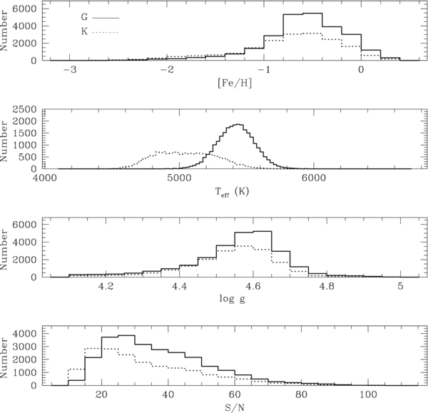
Figure 1. Atmospheric parameters of our sample of around 26,600 G and 18,500 K dwarfs with appropriate S/N and surface gravity. The solid line represents the G dwarfs, and the dotted line the K dwarfs. All of these stars have log g ⩾ 4.1, S/N ⩾ 10 pixel−1, where each pixel is ≈1 Å, and a measured temperature and metallicity.
Download figure:
Standard image High-resolution image3. DISTANCE DETERMINATIONS
Distances are critical both for determining a volume-complete MDF and for examining the behavior of these stars over different regions of the Galaxy. As these stars lack trigonometric parallaxes, we estimate distances by matching each star to YREC isochrones in color and metallicity (Figure 2; An et al. 2009). There are numerous isochrone sets available, such as the Dartmouth (Dotter et al. 2008), BaSTI (Pietrinferni et al. 2004), and Padova isochrones (Girardi et al. 2004). Each isochrone set will predict slightly different behavior along the main sequence, where our stars lie, resulting in systematic changes in distance between sets (Appendix B.4). We also estimate the distances using the photometric parallax relationship of Ivezić et al. (2008, Appendix B.8).
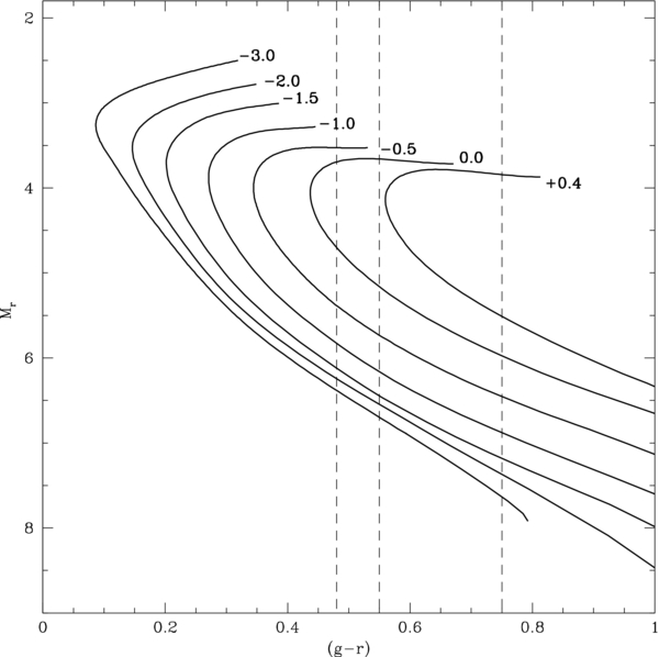
Figure 2. YREC isochrone set for a range of metallicities at an age of 10 Gyr. Each isochrone is labeled with its specific [Fe/H]. The vertical dashed lines show the (g − r) color range for SEGUE G and K dwarfs. These isochrones extend slightly past the main-sequence turnoff to the subgiant branch.
Download figure:
Standard image High-resolution imageWe utilize the YREC isochrones for three main reasons. First, the YREC set is directly calibrated on open and globular clusters, while the other isochrones are not. The Ivezić et al. (2008) photometric parallax relationship is calibrated on the open and globular cluster distances from Harris (1996). Analysis in the interim has found significant variation in these calculated distances, increasing the uncertainty of the calibration, e.g., Table 2 in An et al. (2009). Second, as they are specifically designed to work with SEGUE observations, the YREC isochrones are guided by clusters observed in the SDSS ugriz bands, whereas the Ivezić et al. (2008) photometric parallax relationship must convert from Johnson–Cousins to ugriz, contributing additional distance uncertainty. Finally, the YREC isochrones cover the widest metallicity range of all the different options, from [Fe/H] of −3.0 to +0.4. Both the other isochrones and the Ivezić et al. (2008) photometric parallax relationship extend to only [Fe/H] of −2.5.
3.1. Isochrone Matching
For each star, we select the closest YREC isochrone both above and below the target in [Fe/H]. We limit our isochrones to the main sequence, as we expect all of our targets to be in this evolutionary stage. We also assume an age of 10 Gyr; uncertainties associated with this value are discussed in Appendix B.5. We then match the target's (g − r)0 color to each of the bracketing isochrones, extracting the predicted parameters when the (g − r)0 color matches within 0.001 mag. Using linear interpolation, we determine relationships between stellar parameters, such as the absolute magnitude in ugriz, with respect to [Fe/H]. We then extract isochrone parameters using these relationships and the SSPP estimate of [Fe/H], applying the distance modulus to derive a distance in each filter. Our final value is the mean distance over all of the SDSS filters. We also estimate distances using cubic, rather than linear, interpolation, finding little difference between the stellar parameters determined from these two schemes. Figure 3 shows the distribution of distances for G and K dwarfs.
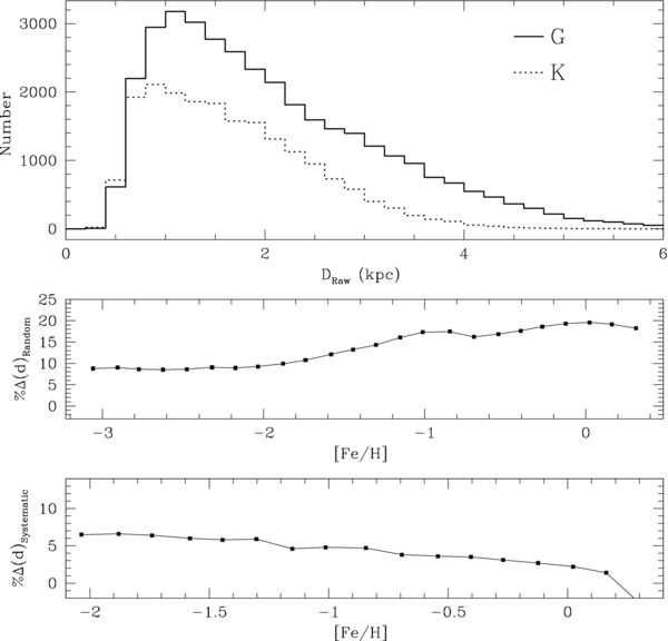
Figure 3. Top plot shows the distribution of G- (solid) and K-dwarf (dashed) distances, calculated by matching to YREC isochrones. The K dwarfs tend to be closer in distance than the G dwarfs, which we expect as they are typically less luminous. The K dwarfs are peaked at a distance of around 0.95 kpc; the G dwarfs peak around 1.25 kpc. The overlapping distance range for K dwarfs and G dwarfs ranges from 1.19 to 1.84 kpc and 1.59 to 2.29 kpc, respectively. The middle plot shows the distance error due to random errors with respect to [Fe/H]. This includes uncertainty from SSPP [Fe/H], photometry, [α/Fe], and isochrone choice. We divide the sample into 25 bins of [Fe/H]; the points represent the mean uncertainty in each bin. The bottom figure shows the systematic uncertainty with respect to [Fe/H], plotted in the same way. This combines the systematic underestimate in distance from assuming that all stars are alone and the overestimate from assigning an age of 10 Gyr to each star. Although we use TRILEGAL for the majority of these uncertainty determinations, we use the SB Galaxy model to constrain the age uncertainty. Although this model covers a wider range of ages, it covers a smaller range of metallicity, going no lower than around −2. At this metallicity, there is a negligible change in distance with a change in age.
Download figure:
Standard image High-resolution image3.2. Distance Uncertainties
There are a number of random and systematic uncertainties, such as the uncertainty in SSPP measurements and undetected binarity, that must be taken into account in our distance estimates. These uncertainties vary with respect to metallicity; small changes in metallicity result in large changes in absolute magnitude at the metal-rich end, whereas there is a smaller effect at the metal-poor end. We use the TRILEGAL 1.4 (Girardi et al. 2005) and Schönrich & Binney (2009a, 2009b) Galaxy models (Sections 6.4.2 and 6.4.1) to estimate the effect of errors in different parameters on our sample. These are discussed at length in Appendix B; the total random and systematic distance errors are shown in Figure 3. The random distance uncertainty originates in the photometric, SSPP [Fe/H], and [α/Fe] errors. There is an additional random distance uncertainty that originates from isochrone choice. Although differences between each isochrone set will create a systematic shift in distance, comparison between the YREC (An et al. 2009), Dartmouth (Dotter et al. 2008), Padova (Girardi et al. 2004), and BaSTI (Cassisi et al. 2006) isochrones reveals that each shifts the distance in a different way. While the Dartmouth set finds larger distances than YREC estimates, those from Padova and BaSTI are smaller. Thus, we treat this variation as a random uncertainty. We find that the total random distance uncertainty ranges from around 18% for stars with [Fe/H] >−0.5 to 8% for more metal-poor stars, dominated by uncertainty in the SSPP [Fe/H] determination.
The systematic uncertainties in distance stem from our age assumptions and the possibility of undetected binarity. Both of these are discussed at length in Appendix B. The most metal-rich stars are likely younger than our assumed age of 10 Gyr. This leads to a systematic shift in distance of −3% for the most metal-rich stars, while the metal-poor stars are largely unaffected. An undetected companion has a comparable effect but goes in the opposite direction; each pair will be systematically shifted by approximately +5% in distance over the entire metallicity range. Conservatively, 65% of all G and K dwarfs are expected to have companions (Duquennoy & Mayor 1991), leading to a total systematic shift of around +3% in distance due to undetected binarity.
We adjust our distances to account for these systematic changes. We assign an offset to each star from age and binarity based on its optimized SSPP [Fe/H], which we then convolve with a Gaussian distribution. As our age assumptions will cause us to overestimate the distances, we subtract the estimated offset from our estimated distance to each star. Assuming that each star is single will cause us to underestimate the distance to approximately 65% of the sample. We randomly select 65% of the sample and increase their distance by the assigned systematic offset from binarity. The systematic uncertainties are much smaller than the random uncertainties at the metal-rich end of the distribution, whereas, due to binarity, they are comparable at the metal-poor end.
3.3. Testing Our Calculated Distances on Globular and Open Clusters
None of our targets have measured parallaxes; thus, we cannot directly confirm that our calculated distances are correct. We instead test our methods against SDSS spectra of stars in open and globular clusters, observed for testing the SSPP determinations and SDSS photometry (Lee et al. 2008b; An et al. 2009; Smolinski et al. 2011). Unfortunately, many of these studies focused on stars past the main-sequence turnoff because they are considerably brighter than dwarfs. We have targets along the main sequence for the clusters M13, M67, NGC 2420, and NGC 6791. This limits us to a metallicity range from [Fe/H] of −1.54 to +0.30.
We select stars from the samples of Lee et al. (2008b) and Smolinski et al. (2011) with well-determined [Fe/H], S/N ⩾ 10, and log g ⩾ 4.1 to ensure that our cluster members are on the main sequence. We do not cut on (g − r)0 color for the globular clusters because this would severely limit our sample size. Furthermore, our distance calculations should hold for any star on the main sequence. As a check, we determined the average distance to the cluster derived from a color-constrained sample to that from the larger main-sequence sample; they match within the expected errors in distance. Thus, a color cut would not significantly affect our distance measurements to these clusters.
The calculated cluster distances are listed in Table 2, in addition to other parameters from Harris (1996), Lee et al. (2008b), Smolinski et al. (2011), and the WEBDA database (Paunzen 2008). A comparison of the clusters and YREC isochrones is shown in Figure 4. The observed stars agree well with the shifted YREC isochrones. The published distances to these clusters vary considerably (Harris 1996; Kraft & Ivans 2003; An et al. 2009; Smolinski et al. 2011); thus, we are pleased with the general agreement we observe from our isochrone-matching method.

Figure 4. Dwarf targets in various open and globular clusters compared to shifted YREC isochrones of comparable age (listed in Table 2). For each cluster, we extract all targets with log g ⩾ 4.1 and calculate their distance using a set of different methods. We have shifted the isochrones according to the mean distance for each cluster from the YREC isochrone technique (in black). The short dashed lines shift the isochrone by the 1σ dispersion of the distance measurements for each cluster. The gray lines show the photometric parallax relationship using the mean SSPP metallicity of the clusters (see Appendix B.8). The vertical long-dashed lines show the SEGUE G- and K-dwarf color cut converted to (g − i). Each plot is labeled with the name of the cluster and the distance modulus used to shift the isochrones. The cluster distances determined using all of our methods are listed in Table 2.
Download figure:
Standard image High-resolution imageTable 2. Cluster Distances
| Cluster | [Fe/H] | E(B − V) | Assumed Age | Literature | Ivezić et al. (2008) Photometric π | YREC |
|---|---|---|---|---|---|---|
| (Gyr) | (kpc) | (kpc) | (kpc) | |||
| M13 | −1.54 | 0.017 | 14 | 7.7 | 7.71 ± 0.78 | 8.01 ± 1.01 |
| M67 | +0.02 | 0.032 | 4 | 0.91 | 0.93 ± 0.10 | 0.87 ± 0.12 |
| NGC 2420 | −0.44 | 0.041 | 2 | 3.09 | 2.73 ± 0.26 | 2.39 ± 0.19 |
| NGC 6791 | +0.30 | 0.117 | 4 | 4.10 | 3.83 ± 0.69 | 3.47 ± 0.52 |
Notes. The parameters and distances determined for the test clusters. The E(B − V) is based on Schlegel et al. (1998), as listed in Lee et al. (2008b). The listed metallicity and literature distances are from Harris (1996) for the three globular clusters and WEBDA for the two open clusters. Note that these metallicity values are slightly different from those found using the SSPP listed in Table 1; the [Fe/H] listed in this table is estimated using the optimized version of the SSPP (Appendix A).
Download table as: ASCIITypeset image
4. CONSTRAINING POSSIBLE BIASES IN THE SEGUE SAMPLE
The selection criteria for G and K dwarfs create numerous biases that affect the sample. For our SEGUE G- and K-dwarf sample to accurately reflect the chemical properties of these spectral types in the Galactic disk, we must ensure that we constrain and account for these observational biases. In this section, we investigate and constrain the possible sources of contamination in the sample and the observational biases induced by the SEGUE target-selection algorithm. We also constrain the effect of each of these errors on our MDF.
4.1. Photometric Errors
Although photometric errors for SDSS photometry are small, typically 2%–3% for each filter, these uncertainties may bump targets in and out of the G- and K-dwarf color and magnitude range. As targets become fainter, their photometric errors increase, making it more likely that a fainter star will be shifted out of the SEGUE color and magnitude criteria due to photometric errors.
Newby et al. (2011) determine that the photometric uncertainties are constant up to r0 of 19.7. The SEGUE target-selection criteria for K dwarfs select stars as faint as r0 of 19 and are thus unaffected by the increasing photometric errors. The G-dwarf magnitude range extends to r0 of 20.2; however, we trim our G-dwarf sample to r0 < 18.45 in order to limit our sample to a magnitude range where the faint end is complete (Section 4.7.2). The photometric uncertainties are thus consistent over the full magnitude range of our G- and K-dwarf sample.
We examine the effect of photometric uncertainty on target selection using TRILEGAL models along SEGUE lines of sight (Section 6.4.2). We estimate the photometric errors in g0 and r0 from the exponential functions of Newby et al. (2011). We then convolve these errors with a Gaussian over multiple iterations to examine how the sample of G- and K-dwarf stars changes with changes in photometry. Approximately 2% of stars are shifted in and out of the sample; those stars removed and inserted into the sample by photometric uncertainties cover a similar range in metallicity space. We examine how the MDF changes over the full metallicity range with this photometric uncertainty, comparing each iteration to the underlying MDF of the model itself. We find that the uncertainty in each bin of the MDF due to photometric errors is on average 6% and should not create any [Fe/H] biases in our derived MDF (see Figure 5).
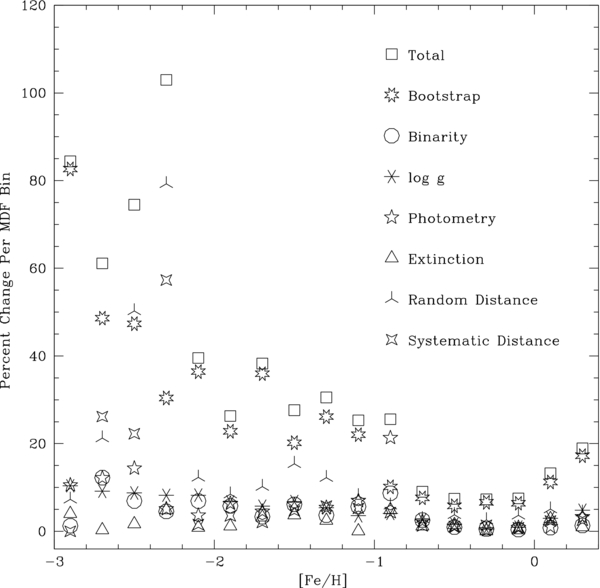
Figure 5. Change in each [Fe/H] bin of the MDF due to different uncertainties. We run a Monte Carlo analysis on the TRILEGAL simulation convolving the expected uncertainty in each of these parameters with a Gaussian to examine how the structure of the MDF changes. At the metal-poor end, the number of stars in each bin is quite small. Thus, the uncertainty from different factors is very large. Typically, uncertainties from our bootstrap analysis and random distance errors dominate. The random distance uncertainties shown here neglect the correlated [Fe/H]-distance error. The MDF uncertainties presented in the following figures and tables reflect the total uncertainty per bin, combining all of the shown errors in quadrature.
Download figure:
Standard image High-resolution image4.2. Undetected Binarity
As the target-selection criteria for G and K dwarfs are based purely on a color and magnitude cut, quantifying the effect of an undetected companion on photometry is critical. Work by Schlesinger et al. (2010) utilized numerical modeling of the SEGUE G- and K-dwarf stars to constrain the effect of binarity on the photometry of the sample. A companion will typically change the (g − r) color measured for a target by 0.01 ± 0.02 mag, less than the uncertainty in SDSS photometry. Undetected companions will also change the photometry in individual filters, affecting distance estimates (Appendix B.6), which we include in the total systematic distance uncertainty.
Although this is a small change in color, it can still shift stars in and out of the (g − r) range for G and K dwarfs. Furthermore, as companions are typically cooler than the primary star, they will make targets appear redder, which may result in undetected binarity preferentially removing the coolest stars from the sample. Schlesinger et al. (2010) investigated the effect of binarity on the properties of SEGUE G and K dwarfs, finding that, assuming that 65% of all G and K dwarfs are in binaries (Duquennoy & Mayor 1991), the addition of a companion will bump around 1% of stars into and 2% of stars out of the (g − r) color criteria. Not only is this a minimal effect, but the numbers of stars shifted in and out are roughly comparable, indicating that binarity will have little effect on the G- and K-dwarf target selection. Using TRILEGAL modeled lines of sight and a modeled population of companions (Appendix B.6), we run a Monte Carlo analysis to estimate the uncertainty in the MDF due to undetected companions. Binarity does not preferentially affect stars of a particular metallicity, with a typical uncertainty of 4% for each MDF bin.
Beyond photometry, Schlesinger et al. (2010) combine their numerical model with synthetic spectra processed through the SSPP to constrain how a secondary will affect the estimates of atmospheric parameters. Effective temperature, which we do not use in our analysis, is the most altered by undetected companions; around 18% of G- and K-dwarf primaries will be shifted by more than 150 K, the reported SSPP uncertainty for S/N of 50. However, undetected binarity has very little effect on the SSPP [Fe/H] estimates. Approximately 99% of the modeled G and K dwarfs undergo shifts of less than 0.2 dex in [Fe/H], less than the expected uncertainty in the SSPP estimates over all S/N. Thus, the effect of binarity on SSPP atmospheric parameters is well within the expected errors, and we do not take it into account.
4.3. Subgiant Contamination
The color and magnitude cuts used to identify our cool dwarfs do not exclusively target main-sequence stars. Subgiants and giants, specifically K giants, can fall into our sample and drastically affect the accuracy of our distance estimates, which assume that all of the targets are on the main sequence. To isolate dwarf stars, we apply a cut on the SSPP log g, limiting it to 4.1 and above. However, the uncertainty of the SSPP surface gravity estimates for stars with S/N of 25 is ±0.4 dex, which may result in evolved stars contaminating the dwarf sample.
We use a threefold approach to examine the extent of the subgiant contamination. First, we employ Galaxy models to estimate the number of subgiants expected to fall in our SEGUE G- and K-dwarf sample. Second, we manufacture a series of synthetic spectra at various evolutionary stages and process them through the SSPP. This allows us to determine if there is a particular region of parameter space where the SSPP has difficulty distinguishing dwarf and giant stars and also constrain how many dwarfs may be lost with a stringent cut in log g. Finally, we use the Mg index to distinguish between giants and dwarfs in our sample (Morrison et al. 2003).
For each line of sight in the SEGUE sample, we model the distribution of stars using TRILEGAL 1.4 (Section 6.4.2). We examine every target in these model distributions with (g − r) in the G/K-dwarf range and log g < 4.2 to determine the size of possible contamination.21 Combining the proportion of subgiants along the TRILEGAL line of sight with the uncertainty in the SSPP surface-gravity measurements, we find that, over all lines of sight, the SEGUE color and magnitude criteria will include a mean of 2% ± 1% subgiants incorrectly identified as dwarfs.
We then combine our population analysis with a study of the SSPP surface-gravity determination using synthetic spectra. As the empirically corrected YREC isochrones used in this study do not extend beyond the main-sequence turnoff, we adopt atmospheric parameters for the giant and dwarf models from the Dartmouth Stellar Evolution isochrones (Dotter et al. 2008) over a range of metallicity (see Appendix B.4 for more details about the isochrones). Breaking the isochrones down into 0.01 mag blocks in color, we manufacture synthetic spectra for both giants and dwarfs using MARCS model atmospheres processed through TurboSpectrum (Gustafsson et al. 2008; Alvarez & Plez 1998). Our MARCS model atmospheres assume solar-scaled abundances, with the solar composition from Grevesse et al. (2007), and plane-parallel geometry. They cover a range in effective temperature from 4700 to 5800 K, −2.5 to +0.5 in [Fe/H], and 1.2–5 in log g. Each of these spectra was adjusted to a range of S/N: 50, 25, and 10. We also analyzed the non-degraded spectra. The spectral synthesis and noise-modeling processes are discussed in more detail in Schlesinger et al. (2010).
Each of these simulated spectra is then processed through the SSPP using the parameter estimates as described in Appendix A. A comparison of the calculated parameters and those input in the models for S/N ∼ 25, the most common S/N for the G- and K-dwarf sample, is shown in Figure 6. At an S/N of 25, the surface gravity tends to be underestimated by 6%, less than the listed SSPP uncertainties. No giants or subgiants will be identified as dwarfs by their log g values. As S/N decreases, the uncertainties in the SSPP parameters increase. At the lowest S/N in our sample, there is a 2% chance of a subgiant being identified as a dwarf by the SSPP and included in our G- and K-dwarf sample. From our population studies of the galaxy models, we expect approximately 2% of stars that fall into our G- and K-dwarf color cuts to be subgiants, and ∼2% of these will be misidentified as dwarfs by the SSPP, resulting in a less than 1% chance that a subgiant will be counted as a dwarf in our sample.
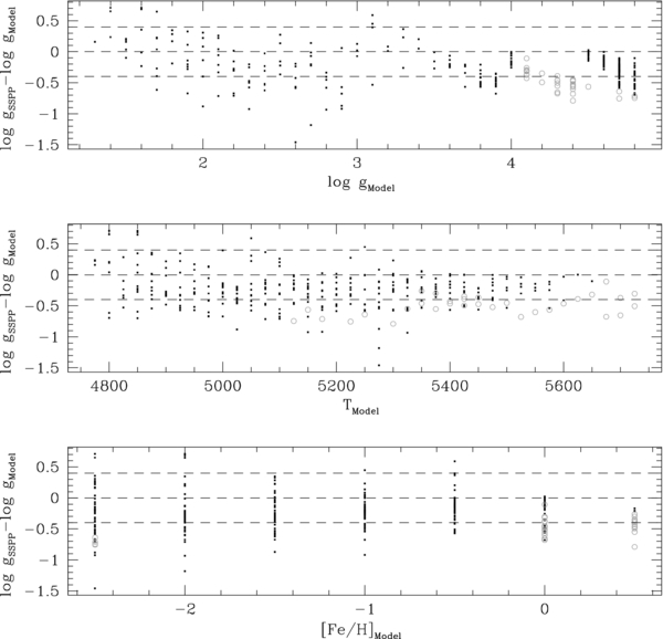
Figure 6. Comparison of the surface-gravity values for the grid of synthetic spectra of dwarfs and subgiants to those determined by the SSPP. These synthetic spectra were degraded to be at an S/N of 25, where the expected SSPP uncertainty in log g is ±0.40 dex. The top panel shows the difference between the model and SSPP-calculated surface gravities with respect to that of the model. The gray open circles show the grid points where modeled stars with dwarf surface gravities have SSPP log g of less than 4.1. The dashed lines show a change in log g of 0 and ±0.4 dex. The SSPP tends to underestimate the surface gravity of these synthetic spectra. There is some structure in Δlog g at the high log g end; this is likely due to the continuum removal processes in the SSPP and is being examined for the SEGUE DR9 public data release. The middle figure shows the change in surface gravity with respect to model effective temperature. Dwarfs misidentified as subgiants tend to be at hotter temperatures. Finally, the bottom panel shows the distribution of Δlog g with respect to model [Fe/H]. Misidentified dwarfs tend to be the most metal-rich stars, although there are a few occurrences at the metal-poor end, where weak lines make it difficult to measure atmospheric parameters. The most metal-rich stars tend to have surface gravities close to the cutoff; even small underestimates can force them from the sample.
Download figure:
Standard image High-resolution imageOur final check on the extent of evolved-star contamination uses the Mg index (Morrison et al. 2003). At a given [Fe/H], giants will have a smaller Mg index value (i.e., less atomic Mg and MgH absorption) than dwarfs. As SEGUE targets K-giant stars in addition to K dwarfs, we focus on this spectral type, calculating the Mg index directly from the SEGUE spectrum. While this index has been calibrated for giants using known open and globular cluster members (Z. Ma et al. 2012, in preparation), we have almost no calibrating observations of known metal-poor dwarfs. Therefore, we identified stars from our sample that were very likely to be dwarfs using a reduced proper-motion criterion (Lépine & Gaidos 2011). Binning in metallicity, we isolate a control sample of "true" dwarf stars by specifying that the total proper motion must be greater than 20 mas yr−1, and the r0 magnitude reduced proper motion is greater than 13. We then examine the spectra of targets where the Mg index is lower than expected for the true dwarfs, e.g., they are in the parameter space of evolved stars. This visual inspection consisted of the following three tests:
- 1.the strength of the Mg feature in non-continuum-corrected SEGUE spectra (Morrison et al. 2000);
- 2.
- 3.
These three tests are valuable luminosity discriminants and isolate subgiant and giant stars masquerading as dwarfs in the sample. Our visual analysis indicates that less than 1% of the total sample of SEGUE K dwarfs are actually evolved stars, confirming that subgiant and giant contaminants have a negligible presence in our sample for both spectral types. We do not take this negligible contamination into account.
Our analysis of synthetic spectra indicates that the SSPP tends to underestimate surface gravity, which prevents subgiants from entering the sample. However, it also means that a number of dwarf stars will fall out of the sample when it is selected using a surface-gravity cut. In particular, we will preferentially lose high-metallicity stars, as these have surface gravities closer to the boundary of log g. We run a Monte Carlo analysis to examine how uncertainties in surface gravity will affect the MDF. We model each SEGUE line of sight with the TRILEGAL Galaxy model (Section 6.4.2), selecting G- and K-dwarf "spectroscopic" targets based on SEGUE photometric criteria. We then determine the "true" MDF for this sample. Next, we vary the modeled surface-gravity values, convolving them with a Gaussian error distribution with σ of 0.6 dex, the largest possible SSPP uncertainty. We then compare the MDF of these modified samples to the original, to estimate the MDF uncertainty from SSPP log g errors. For [Fe/H] ⩾−1.0, the change in each MDF bin is around 3%. Below this metallicity, the percent change is higher, around 10%, due to the small-number statistics of this portion of the simulated distribution (Figure 5). These are much smaller than the expected MDF uncertainties from bootstrapping alone (Section 5.2) and do not induce a bias in the metallicity distribution.
4.4. Extinction
Although the lines of sight in SEGUE typically probe above and below the plane of the Galaxy, undergoing small amounts of extinction, this small amount of reddening can affect SEGUE target selection, which is based on color and magnitude. We determine the extinction per plate using the r-band extinction from the Schlegel et al. (1998) maps for every object listed as a star.22 All but 11 of the plates (1888, 2052, 2179, 2300, 2334, 2335, 2623, 2669, 2679, 2680, and 2805) have extinction less than 0.5 mag in r and E(g − r) of less than 0.2 mag. Reddening cuts remove around 6% of the sample.
Although many of the lines of sight have minimal extinction, there is still a danger that reddening will bias the G- and K-dwarf sample. Closer stars will have undergone less extinction than those farther away; using the extinction corrections from Schlegel et al. (1998) may make close-in, metal-rich stars appear artificially blue, leading to inaccurate distance estimates and bumping stars in and out of the G- and K-dwarf SEGUE sample. This should be a minimal effect, as our stars have a minimum |Z| of 0.2 kpc, beyond the expected scale height of 0.14 kpc for dust in the disk (Mendez & van Altena 1998).
We use the sample of Cheng et al. (2012) to examine the accuracy of Schlegel et al. (1998) extinction estimates with respect to distance. Cheng et al. (2012) calculated the extinction for a sample of SEGUE main-sequence turnoff stars by matching the isochrone-predicted (g − r) color, found using the SSPP parameters, to the observed. Unlike the Schlegel et al. (1998) values, this reddening calculation does not assume that each star lies behind the full amount of line-of-sight dust. For their four lines of sight with E(g − r) less than 0.2 mag, similar to our own, the Cheng et al. (2012) isochrone extinction is comparable to the Schlegel et al. (1998) values over the full distance range (J. Cheng 2012, private communication). Thus, in areas of generally low extinction, using Schlegel et al. (1998) extinction estimates will not induce a bias in our sample against metal-rich stars by preferentially removing nearby stars.
As with photometric errors and undetected binarity, extinction can also artificially shift stars in and out of the G- and K-dwarf color and magnitude range. Specifically, if extinction is overestimated, bluer stars will be scattered in and red stars out of the color range. To constrain these effects, we simulate the distribution of reddening values at a range of extinctions, using the main-sequence turnoff stars from Cheng et al. (2012), on TRILEGAL Galaxy models along each SEGUE line of sight. Modeling the extinction with respect to distance along each SEGUE line of sight, we examine how the G- and K-dwarf sample changes. Although reddening does shift stars in and out of the G- and K-dwarf color range, it does not preferentially remove stars from a certain metallicity space. The uncertainty per metallicity bin in the MDF due to extinction is typically around 2% (see Figure 5).
4.5. Volume Completeness
Our G- and K-dwarf sample covers a wide range of metallicities. Metal-rich stars are brighter than metal-poor ones for a given (g − r) color. Thus, the volume coverage of the sample varies with respect to metallicity for the same magnitude range. At the bright end, metal-rich stars will saturate; at the faint end, metal-poor stars are not sufficiently luminous to be observed by SEGUE. To ensure that our SEGUE sample and MDF are not biased with respect to chemistry due to the metallicity-dependent volume coverage, we specify distance limits for our sample.
We examine the YREC isochrones for a metallicity of [Fe/H] of +0.4 and −3.0, extracting the r-band magnitudes for targets with (g − r) of 0.48, 0.55, and 0.75. Using the distance modulus, we calculate the maximum and minimum distance for both spectral types over a range of metallicity. For K dwarfs, the distance range for SEGUE volume completeness is from 1.19 to 1.84 kpc; for G dwarfs, the distance range is from 1.59 kpc to 2.29 kpc. Note that these distances utilize adjusted r-magnitude limits for the G and K dwarfs, as described in Section 4.7.2. In this paper, we refer to the distance range from 1.59 to 1.84 kpc as the overlap distance range. These distance limits are used in comparisons between the G- and K-dwarf sample. For analysis of an individual spectral type, we use the larger distance range associated with either G or K dwarfs. We refer to this range as the spectral-type distance range.
Random and systematic uncertainties in distance will shift stars in and out of the overlap range. We estimate the effect of these changes in distance on our MDF with a Monte Carlo analysis of the TRILEGAL simulation (Section 6.4.2). Each star is assigned a typical percent change in distance from random and systematic effects, which is then convolved with a Gaussian over multiple iterations. We use a random distance uncertainty from errors in photometry, [α/Fe], and isochrone choice; the systematic uncertainties originate in age and binarity assumptions. For [Fe/H] ⩾−2.0, variation in the systematic distance will change each MDF bin by around 3%. The number of stars at the metal-poor end is very small, leading to larger uncertainties, on average 35% (see Figure 5). The random distance uncertainties have a larger effect than systematic uncertainties, changing each bin by approximately 7% and 40% at the metal-rich and metal-poor ends, respectively. These distance errors are included in our total MDF uncertainties.
We do not include the change in distance due to SSPP [Fe/H] uncertainties as part of our random distance uncertainty, as these properties are strongly correlated. Overestimating the metallicity will lead to an overestimate in distance, and vice versa. Uncertainties from [Fe/H] will both broaden the true metallicity distribution and shift stars in and out of the sample due to distance cuts. To estimate the size of these effects, we perform a Monte Carlo analysis along the TRILEGAL modeled lines of sight. For each modeled G- and K-dwarf star, we vary the [Fe/H], convolving the SSPP errors with a Gaussian, and adjust the corresponding distance to account for this change in metallicity. We then compare the different Monte Carlo iterations to the true distribution (see Figure 7). The cumulative distributions of G and K dwarfs indicate that the [Fe/H] and distance error broadens the MDF of the TRILEGAL model. To quantify the extent of this effect, we estimate the slope of the cumulative distribution between fractions 0.25 and 0.75. Larger uncertainties in [Fe/H] will manifest in larger negative slopes in this portion of the cumulative distribution. For the true model distribution, the slope is around −0.6 dex−1, whereas it increases to −1.0 dex−1 when we factor in σ[Fe/H]. We list the broadened slopes for both spectral types in Figure 7. Thus, uncertainties will cause us to measure a broader, by slightly less than a factor of two, version of the true underlying distribution.
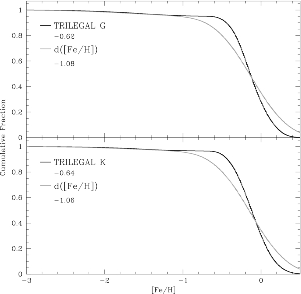
Figure 7. Comparison of the true cumulative metallicity distribution from the TRILEGAL model to a distribution that includes the correlated uncertainties in [Fe/H] and distance. We simulate the G (top, black) and K (bottom, black) dwarfs in SEGUE using a TRILEGAL model. Using a Monte Carlo analysis, we factor in the uncertainties in [Fe/H] and the resulting change in distance. This broadens the metallicity distribution a significant amount, as indicated by the gray d([Fe/H]) lines. We estimate the slopes of these distributions between a cumulative fraction of 0.25 and 0.75; they are listed in the figure. This change estimates the amount of broadening in our MDFs caused by errors in metallicity.
Download figure:
Standard image High-resolution image4.6. Evolutionary Effects
To derive a complete chemical history of the Galactic disk, we must ensure that no stars have evolved off of the main sequence, as this would bias our SEGUE sample against metal-rich stars. Figure 2 shows the YREC isochrone set at an age of 10 Gyr for a range of metallicities (An et al. 2009). The G- and K-dwarf SEGUE color-cut regions are indicated. The most metal-rich 10 Gyr isochrones, calibrated to NGC 2862 and NGC 6791, have the main-sequence turnoff before reaching the red edge of the color range for the SEGUE G dwarfs. At younger ages, these metal-rich isochrones cover the entire G (g − r) range, indicating that there is a chance we are losing old, metal-rich G dwarfs due to evolutionary effects.
To investigate the extent of this evolutionary effect, we compare the metal-rich samples of the two spectral types. Over the overlapping distance range for both G and K dwarfs, approximately 3% ± 1% of G dwarfs have metallicities greater than 0. Around 10% ± 3% of K dwarfs are this metal-rich. Between [Fe/H] of −0.3 and 0, the G- and K-dwarf distributions are consistent with one another. This indicates that our selection criteria lose metal-rich ([Fe/H] ⩾ 0) G dwarfs older than 5 Gyr.
4.7. Correcting for Metallicity Biases from Target Selection
For our G- and K-dwarf sample to accurately reflect the chemical properties of these spectral types in the Galactic disk, we must ensure that we constrain and account for the different metallicity biases induced by SEGUE target selection.
There are three metallicity biases in the SEGUE G- and K-dwarf sample that we correct for:
- 1.Other SEGUE target categories that are biased toward metal-poor stars overlap the color range of the SEGUE G and K dwarfs, biasing the color-selected sample in metallicity.
- 2.SEGUE has the same limited number of spectroscopic fibers for each line of sight, regardless of its stellar density.
- 3.The G- and K-dwarf color cuts select a range of stellar masses, and thus a subset of the mass function, that varies with metallicity.
To correct for the effects of target selection, we compare the spectroscopic sample along each individual line of sight to the photometric sample. For each pointing and target category, we scale the spectroscopic distribution in r0 such that it matches the underlying r0 magnitude distribution of all of the stars that could have been observed spectroscopically. Our sample consists of 152 different lines of sight, each with a different distribution of spectral types and number of stars. Thus, we must correct for the target-selection biases on a plate-by-plate basis.
For each bright and faint plate combination, we extract every possible photometric stellar target within the plate radius that passes the G- and K-dwarf color and magnitude criteria, whether or not it was observed spectroscopically.23 We then match each of these stars with SEGUE spectroscopy. Matching photometry and spectroscopy is a non-trivial task because some plates were observed multiple times and many stars were repeated, some unintentionally, as geometric overlaps from multiple plates, and others as purposeful re-observations. Additionally, targets from SEGUE were occasionally observed again as part of SEGUE-2. We removed all duplicate spectroscopic observations, selecting the highest S/N observations using the sciencePrimary parameter. We also trimmed our spectroscopic sample to eliminate any poor observations, removing all targets that have S/N < 10, an incalculable [Fe/H], or specific warning flags (Section 2.2). These targets remain within the photometric sample, as they are simply counted as stars that do not have spectra. For each spectroscopic target that fulfills the G- or K-dwarf color and magnitude cut, we determine three weights: target type, r magnitude, and mass function. As we do not know the log g of targets assigned SEGUE fibers in advance, we calculate these weights for all usable spectroscopic G and K stars. We trim our sample in surface gravity when we calculate our unbiased MDFs.
4.7.1. Target-type Weights
The simple selection criteria of SEGUE G and K dwarfs overlap with the criteria for other different SEGUE targets. SEGUE categories often focus on specific ranges in parameter space, such as stars with low metallicity or small proper motions. Targets that fulfill multiple target-type criteria have multiple opportunities to be assigned a spectroscopic fiber. This leads to an overabundance of other stellar categories in the G- and K-dwarf sample. For example, the SEGUE low-metallicity star and K-giant categories use a ugr selection based around UV excess to identify targets, overlapping with the G- and K-dwarf criteria in (g − r). These target categories will bias the SEGUE G- and K-dwarf sample toward metal-poor stars (Figure 8).
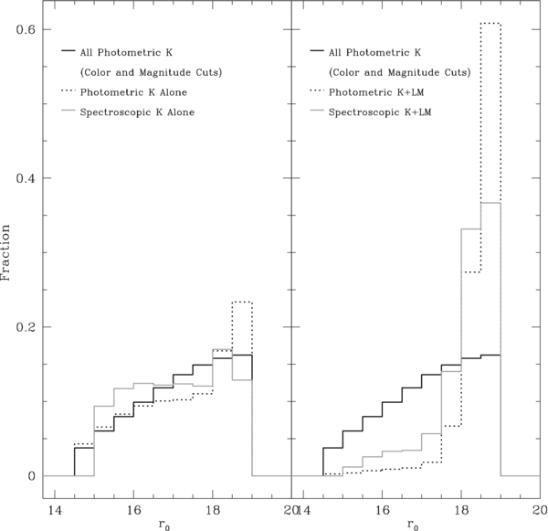
Figure 8. SEGUE G- and K-dwarf sample overlap with other SEGUE target categories, biasing them in metallicity space. The solid black line shows the r0 distribution of all photometric stars along the SEGUE lines of sight that meet the color and magnitude criteria of a K dwarf. On the left-hand side, we show the distribution of all photometric stars that meet only the criteria of a K dwarf as the dotted line. We also present the r0 distribution of all SEGUE spectroscopic observations that meet only the criteria of a K dwarf. In contrast, on the right-hand side we show the photometric and spectroscopic sample of stars that meet the criteria of a K dwarf and a low-metallicity target. It has a significantly different distribution than the K-dwarf targets alone.
Download figure:
Standard image High-resolution imageEvery stellar target observed photometrically by SDSS is labeled with the SEGUE categories it fulfills. Any individual star may pass the selection criteria for more than one target type and is then labeled as being a candidate for more than one SEGUE spectroscopic sample. We compare the number of stars identified as photometric candidates for each target type and each combination of target types (i.e., a K-dwarf and a low-metallicity target) with the number of those candidates that have good spectra, as defined in Section 2. We assign a "target-type weight" such that the two distributions match. This removes biases due to the overlapping target types in SEGUE, be they over- or undersampled by the spectroscopic fibers, ensuring that the type of stars probed by SEGUE reflects that of the underlying photometric sample.
Figure 9 shows the mean target-type weight with respect to [Fe/H] for both spectral types. This correction reduces the proportion of metal-poor stars for both spectral types. Otherwise, the K-dwarf weights are typically much higher than those for G-dwarf stars. There is also more variation with [Fe/H]. While the selections of metal-poor and K-giant stars in the G-dwarf color region are relatively inefficient, the K-dwarf color selection is more contaminated with stars from other categories, biasing the metallicity structure. At [Fe/H] ⩾−0.5, the K dwarfs have a target-type weight of around 2.2, indicating that metal-rich K dwarfs are underrepresented by a factor of two. In contrast, the target-type weight for metal-rich G dwarfs is approximately 0.7, suggesting that they are oversampled in SEGUE. Below [Fe/H] of −1.5, the target-type weights are around 0.7 and 0.4, for K and G dwarfs, respectively. Our calculated target-type weights will be available with SDSS DR9.
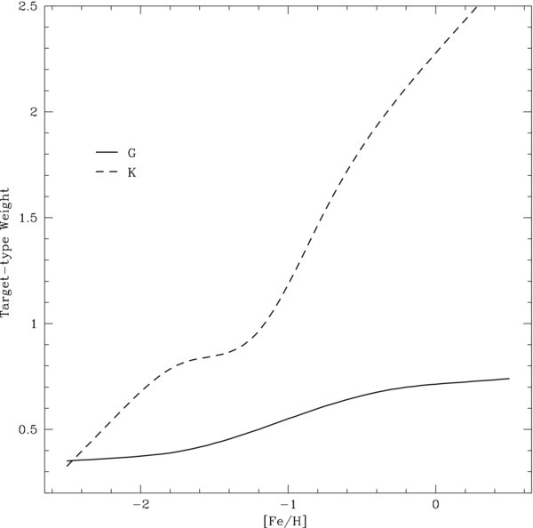
Figure 9. Comparison of the mean target-type weight with respect to [Fe/H] for G (solid line) and K dwarfs (dashed line). There are fewer SEGUE fibers devoted to K-dwarf targets along each line of sight, making the sample more contaminated by stars assigned fibers for other stellar categories. The target-type weights account for this by scaling down the proportion of metal-poor stars and scaling the metal-rich end of the distribution. The variation in target-type weights for G-dwarf stars is much smaller, as it suffers less from target-selection biases.
Download figure:
Standard image High-resolution imageLee et al. (2011b), Bovy et al. (2012b), and Liu & van de Ven (2012) determine their stellar sample by extracting only stars assigned spectroscopic fibers as G dwarfs. This greatly diminishes the size of the spectroscopic sample. Furthermore, although this method does not explicitly include stars targeted as low-metallicity, that does not make it unbiased in [Fe/H]. For example, if all of the low-metallicity stars along a particular line of sight receive SEGUE fibers as low-metallicity targets, none will be included in the G-dwarf sample, regardless of whether or not they fulfill the criteria, creating a bias toward metal-rich stars. Fortunately, the G-dwarf sample is significantly less affected by the metallicity bias of SEGUE target selection (Figure 9).
4.7.2. r-magnitude Weights
SEGUE probes each line of sight with a limited number of fibers; the survey cannot spectroscopically observe every target in a field. Lower latitude pointings are closer to the plane of the Galaxy, have many more stars, and tend to be more metal-rich than high-latitude lines of sight. SEGUE assigns the same number of fibers to each line of sight, regardless of latitude and stellar density. This leads to a bias against metal-rich stars in the observed MDF of the full survey. Furthermore, to accurately measure the properties of the Milky Way, we must ensure that our spectroscopic sample reflects the apparent-magnitude distribution of the underlying photometry along each line of sight.
To calculate these "r-magnitude weights," we separate the spectroscopic and photometric sample into G and K dwarfs based on (g − r)0 color. We examine the distribution in r0 magnitude for each individual spectral type, binning up the spectroscopic and photometric targets in 0.5 mag bins from r0 = 13 to 21.5 mag. These bin sizes ensure that we typically have at least one spectroscopic target associated with each group of photometric stars. While the r-magnitude weights change when specifying a smaller bin size in r0, the MDF changes very little, well within the expected uncertainties for each bin of [Fe/H]. We compare the number of spectroscopic targets in each bin to the number of potential targets in the photometric sample. The inverse of this ratio is the weight assigned to each spectroscopic target with a measurable [Fe/H] and S/N ⩾ 10 to recreate the parent photometric distribution. This quantity, which we refer to as the r-magnitude weight, accounts for the fact that SEGUE does not have unlimited fibers.
Examining the faint end of the G-dwarf sample reveals that there are very few usable spectroscopic targets with S/N ⩾ 10 at the faintest magnitudes. However, there are often many photometric targets at these faint magnitudes, leading to large r-magnitude weights and anomalous spikes in the MDF. To determine the true magnitude range of the usable spectroscopic sample, we examine the cumulative distribution of spectroscopic targets in r0 for each plate. We find that 85% of all spectroscopic G dwarfs have r0 ⩽ 18.45. By setting 18.45 as our faint magnitude limit for G dwarfs, we avoid anomalous weighting. The magnitude criteria for K dwarfs in SEGUE are significantly more conservative than those for the G dwarfs, extending to r0 of 19; thus, the K-dwarf sample does not have the same faint-end problem.
As K-dwarf stars are more frequent than G-dwarf stars, and sampled more sparsely in SEGUE, these targets tend to have higher r-magnitude weights. Both G- and K-dwarf stars also have high r-magnitude weights for lines of sight that probe lower Galactic latitudes. For G dwarfs with [Fe/H] ⩾−0.5, the typical r-magnitude weight is around 13; the typical weight for K dwarfs is around 15. This value decreases to 8 and 11 for G and K dwarfs below [Fe/H] of −1.5, respectively. As with the target-type weights, the r-magnitude weights will be available to the public as part of SDSS DR9.
4.7.3. Mass-function Weights
The (g − r)0 cut that defines the G- and K-dwarf targets corresponds to different mass ranges for each metallicity. For example, the G-dwarf color cut isolates stars with mass near 0.7 M☉ for [Fe/H] of −1.0 and near-solar mass stars for solar metallicity. Mass functions for the Galaxy predict a larger number of less massive stars; thus, the color cut of SEGUE will result in a metallicity bias in our sample. Previous studies (e.g., Jørgensen 2000) discarded stars to find a mass range over which their samples were reasonably complete, but, due to our narrow color range, this would drastically limit our sample. The masses probed by our color and metallicity range are typically from 0.5 to 1.0 M☉ but do not necessarily overlap for each metallicity bin. As this is not a large range in mass, we expect the metallicity bias introduced by our color cuts to be a small effect compared to other observational biases that affect the sample.
We employ the TRILEGAL 1.4 model (Section 6.4.2), which utilizes a Chabrier mass function, to estimate this effect. We extract two samples from the model for each individual line of sight. The first sample has the same color and magnitude range as the G- or K-dwarf sample and is restricted to stars with log g ⩾ 4.1, to identify main-sequence stars. We bin this sample in metallicity for each spectral type and examine the distance range the sample covers at each [Fe/H]. The second sample is also limited to stars on the main sequence and in the G or K magnitude range. However, rather than a color cut, we extract all stars with masses between 0.5 and 0.6 M☉ that fall within the same distance range of stars in the color cut. This ensures we are comparing the two samples over the same volume of space. For each metallicity bin, we compare the number of stars that fulfill the color criteria to the number of targets with masses between 0.5 and 0.6 M☉ within the same volume. This ratio indicates how much to scale each metallicity bin of the G or K dwarfs to simulate sampling a consistent portion of the mass function over the entire metallicity range. As the mass function varies slightly from plate to plate, we calculate these weights for each SEGUE pointing.
We also calculate mass weights based on the Schönrich & Binney (2009a, 2009b) Galaxy models (SB), which utilize a Salpeter IMF (Salpeter 1955), to examine how much these values will vary with different assumptions about the mass function (Section 6.4.1). The distribution of weights from the SB models is comparable to the mass-function weights derived from the TRILEGAL simulation; using SB values rather than TRILEGAL has a negligible effect on the metallicity distribution. The TRILEGAL models cover a wider metallicity range than those of Schönrich & Binney (2009a, 2009b), reaching lower metallicities, so we use these weights throughout our analysis.
As with the other two weights, the mass-function weights decrease the proportion of metal-poor stars. However, in contrast to the weights for overlapping categories and spectroscopic sampling, the mass-function weights are not large; above [Fe/H] of −0.5, both G and K dwarfs have a typical mass weight of around 1.0. For metal-poor stars ([Fe/H] ⩽−1.5), the typical mass weight is 0.7 for G dwarfs and 0.9 for K dwarfs. These values will not be released as part of SDSS DR9, as other groups will have their own preferred mass function.
4.7.4. Testing the Target-selection Weighting on Galaxy Models
Figure 10 shows the original and adjusted MDF for G and K dwarfs over all the SEGUE lines of sight for the spectral-type distance range. As explained in Sections 4.7.1–4.7.3, the corrections for SEGUE target-selection biases significantly affect the MDF, increasing the metal-rich end.
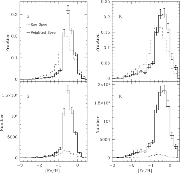
Figure 10. Raw and weighted MDF for the G (left) and K (right) dwarfs. The raw spectroscopic sample is the dashed line. The sample adjusted for target-type, r-magnitude, and mass-function weights is the solid line. The error bars on the solid line reflect the error in each bin based on our total MDF uncertainty, combining our bootstrap analysis with other errors (Section 5.2). Both samples are limited to their spectral-type distance ranges, as described in Section 4.5. Note that the corrections associated with the target-selection scheme boost the metal-rich end of the distribution.
Download figure:
Standard image High-resolution imageTo ensure that our weighting algorithm appropriately removes biases from target selection, we test it on a series of modeled lines of sight from the TRILEGAL 1.4 theoretical Galaxy model (Section 6.4.2). We analyze each TRILEGAL line of sight as a photometric sample for SEGUE target selection, labeling all modeled stars that meet the color and magnitude criteria of the SEGUE G- and K-dwarf categories. We randomly select 375 G and 95 K dwarfs for each line of sight as our "spectroscopic" observations, weighting this mock SEGUE sample according to the methodology discussed in Sections 4.7.2 and 4.7.3. We then compare the weighted parameter distribution in [Fe/H] in two ways to that of the underlying sample. First, we compare the "spectroscopic" sample, weighted in target type and r magnitude, to the modeled photometric sample (see Figure 11). The combination of these two weights recreates the metallicity distribution for all modeled stars that fulfill the G- and K-dwarf criteria. This suggests that our photometry-based weighting techniques allow us to examine the metallicity structure of the underlying stellar populations in the disk using our spectroscopic sample.

Figure 11. Test of the target-type and r-magnitude weighting system on the TRILEGAL Galaxy model. The dashed line represents the distribution of a randomly selected subsample of G and K dwarfs representing the SEGUE spectroscopic sample, which we refer to as the "raw spectroscopic." The gray line is the distribution of every modeled star that meets the G- and K-dwarf photometric criteria. Finally, the solid black line is the distribution of the spectroscopic sample once we have weighted it in r magnitude and target type. The top figure shows the numerical distribution of the three samples; the good match between the weighted spectroscopic and photometric distributions indicates that our technique accurately corrects for SEGUE target-selection biases. The bottom figure shows the fractional distribution of the three samples. The "raw" spectroscopic sample is biased toward metal-poor stars, but our weighting scheme corrects for this.
Download figure:
Standard image High-resolution imageOur second comparison, shown in Figure 12, uses the target-type, r-magnitude, and mass-function weights to recreate the distribution of all stars that meet the G- and K-dwarf magnitude criteria and fall in a uniform mass range. The underlying photometric sample that we tested the target-type and r-magnitude weights on is slightly biased in mass, as explained in Section 4.7.3. The top plot compares a (g − r) color cut to a mass cut in metallicity space, where both samples cover the same volume for each individual metallicity bin. There is little difference between the two distributions. The bottom plot indicates that the color cut manifests as a bias toward metal-poor stars. Our target-selection weights account for this, removing the color-cut effect such that it appears that our sample is extracted from a uniform portion of the mass function. We also tested our target-selection corrections on the Galaxy model of Schönrich & Binney (2009a, 2009b, SB; Section 6.4.1), with similar results.
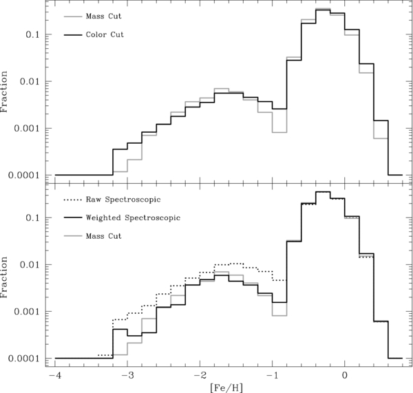
Figure 12. Test of the mass-function weights on the SEGUE lines of sight modeled with TRILEGAL. The top figure compares the effect of a color cut on the metallicity distribution to a mass cut. The color cut extracts all stars within the magnitude and (g − r) range of the SEGUE G and K dwarfs, shown in black. The mass cut selects all stars within the magnitude range with masses between 0.5 and 0.6 M☉, shown in gray. Each metallicity bin of the two samples probes the same volume of space. The two distributions are quite similar, although there are some discrepancies at the metal-poor end. The bottom row tests our weighting scheme. The gray distribution remains the same as in the top plot. The additional distributions represent a randomly chosen G/K-dwarf subsample to represent SEGUE spectroscopy (dashed) and this distribution weighted in target type, r magnitude, and mass function (black). The weighted distribution scales the raw spectroscopic down at the metal-poor end and boosts the metal-rich end, such that it simulates isolating a uniform portion of the mass function.
Download figure:
Standard image High-resolution image4.8. Summary of the G- and K-dwarf Sample
Our SEGUE sample consists of 16,847 K dwarfs with S/N ⩾ 10, surface gravities larger than log g = 4.1, appropriate r0 magnitudes, and E(g − r) less than 0.2 mag. This sample has −3.4 ⩽ [Fe/H] ⩽ 0.6, 4.1 ⩽log g ⩽ 5.0, and 4150 K ⩽ Teff ⩽ 6315 K. It contains stars with distances from 0.3 to 5.8 kpc and covers Galactic radii from 4.8 to 13.4 kpc and heights from the plane up to ±4.0 kpc. We have 24,270 G dwarfs with the appropriate S/N, surface gravity, extinction, and r0. This sample ranges from [Fe/H] of −3.1 to 0.6, surface gravities up to 5.0, and effective temperatures from 4210 to 6300 K. It extends to larger distances than the K-dwarf sample, from ∼0.4 to 10.2 kpc, covering from 3.7 to 16.5 kpc in Galactic radius and −7.7 to 9.7 kpc in height above the Galactic plane.
We have performed the first complete analysis of the different possible biases in this SEGUE sample. The color and magnitude selection criteria of the two categories result in a sample that is quite clean, with few stars of inappropriate color being shifted into the sample by photometric errors or undetected binarity. We also remove lines of sight from our sample with E(g − r) greater than 0.2 mag and establish that uncertainties in the Schlegel et al. (1998) extinction measurements have little effect on our distance estimates.
We also constrain how stars of different evolutionary phase affect our sample. Combining an analysis of log g with MgH and Galaxy models, we determine that the SEGUE G and K dwarfs will have a negligible amount of contamination from evolved stars. We will lose old, metal-rich stars from the G-dwarf sample due to evolution; our (g − r) color cut biases the G-dwarf sample against stars with [Fe/H] ⩾ 0.
We estimated the effect of different uncertainties in the G- and K-dwarf sample on the MDF (see Figure 5). The uncertainties are dominated by distance errors, both random and systematic. None of the various uncertainties, from photometric errors to undetected binarity, induce a bias in the metallicity of the sample. In our MDF, we include every different source of uncertainty in the structure, combining them in quadrature (Section 5.2).
Although issues ranging from surface gravity to extinction have little effect on our derived MDF, the target-selection algorithm of SEGUE does bias the sample in metallicity space, favoring metal-poor stars. The same number of stars are observed in fields at low Galactic latitude, which have a high stellar density and are dominated by high-metallicity stars, as in those at high Galactic latitude, where the stellar density is much lower and the stars are primarily metal-poor. Thanks to the quantitative target-selection algorithm of SEGUE, we have both quantified and corrected for these different biases using a series of weights. The uncertainties from these values are integrated into our MDF uncertainties via a bootstrap analysis (Section 5.2).
5. THE METALLICITY DISTRIBUTION FUNCTIONS OF G AND K DWARFS OVER THE DISK
5.1. MDF of the Disk as a Whole
For each spectral type, we determine the distribution of stars with respect to metallicity and then apply our target-selection weights such that the distribution reflects the chemical structure of the underlying disk population. This allows us to improve on previous analyses, namely, photometric metallicity estimates, limited volume coverage, observational biases, and/or small sample size. Figures 10 and 13 show the total MDF for G and K dwarfs over the spectral type and overlapping distance ranges, respectively. This is the first unbiased MDF using spectroscopic metallicities over a substantial volume of the disk for both G and K dwarfs.

Figure 13. Comparison of the G- (black) and K-dwarf (gray) MDFs. Both samples are limited to distances between 1.59 and 1.84 kpc. The error bars are based on our total MDF uncertainty, combining a bootstrap analysis over 500 iterations with other sample uncertainties (Section 5.2). The two samples cover a similar metallicity range and peak at approximately the same value. At low |Z|, K dwarfs have more metal-rich stars, due to evolutionary effect. At high |Z|, they also have more metal-poor stars. This results in a broader distribution than observed for the G dwarfs over all |Z|.
Download figure:
Standard image High-resolution imageThese MDFs provide information about the chemical structure of the disk from approximately 0.2 to 2.3 kpc above and below the plane of the Galaxy, and from Galactic radii of around 6–11 kpc (Figure 14). The MDF of both G and K dwarfs ranges from metallicities of around −2.5 to +0.4. The distributions peak at around [Fe/H] of −0.4 to −0.6, indicating that the sample has a large population of thick-disk stars, in addition to substantial contributions from the thin disk with [Fe/H] = −0.2 (Gilmore & Wyse 1985; Wyse & Gilmore 1995; Chiba & Beers 2000). Unlike the dwarf stars in the GCS and RAVE surveys, the SEGUE sample has coverage of both the in situ thin and thick disks. Thus, our total MDFs reflect the overall disk properties, rather than an individual component of the Milky Way disk. Detailed information about these distributions for further analysis is available in Table 3.

Figure 14. Spatial positions of our G (black) and K (red) dwarfs. The Geneva–Copenhagen Survey (GCS) sample of stars is shown in blue (Nordström et al. 2004; Haywood 2008; Casagrande et al. 2011). The G dwarfs are limited to distances between 1.59 and 2.29 kpc, whereas K dwarfs fall between 1.18 and 1.84 kpc, based on the magnitude limits of SEGUE. This reduces our stellar sample to 5407 K and 7834 G dwarfs. Our sample probes the disk both toward and away from the Galactic center and above and below the Galactic plane, with the line-of-sight structure of SEGUE clearly visible. The GCS sample is limited to the solar neighborhood, with distances typically less than 200 pc.
Download figure:
Standard image High-resolution imageTable 3. Total Metallicity Distribution Functions of G and K Dwarfs over Different Distance Ranges
| [Fe/H] | G Dwarfs | K Dwarfs | ||||||||||||||
|---|---|---|---|---|---|---|---|---|---|---|---|---|---|---|---|---|
| 1.59 ⩽ d ⩽ 2.29 kpc | 1.59 ⩽ d ⩽ 1.84 kpc | 1.18 ⩽ d ⩽ 1.84 kpc | 1.59 ⩽ d ⩽ 1.84 kpc | |||||||||||||
| Raw | Weighted | Raw | Weighted | Raw | Weighted | Raw | Weighted | |||||||||
| +0 | +0 | +0 | +0 | +1 | +6 | +0 | +0 | |||||||||
| −3.3 | 0 | 0 | 0 | 0 | 1 | 7 | 0 | 0 | ||||||||
| −0 | −0 | −0 | −0 | −1 | −7 | −0 | −0 | |||||||||
| +1 | +1 | +0 | +0 | +2 | +49 | +2 | +50 | |||||||||
| −3.1 | 2 | 1 | 0 | 0 | 6 | 25 | 4 | 18 | ||||||||
| −1 | −1 | −0 | −0 | −3 | −13 | −2 | −11 | |||||||||
| +2 | +15 | +0 | +0 | +3 | +17 | +2 | +8 | |||||||||
| −2.9 | 3 | 15 | 0 | 0 | 5 | 22 | 2 | 6 | ||||||||
| −2 | −10 | −0 | −0 | −2 | −10 | −1 | −4 | |||||||||
| +3 | +10 | +2 | +6 | +5 | +83 | +4 | +75 | |||||||||
| −2.7 | 8 | 26 | 4 | 10 | 16 | 58 | 3 | 18 | ||||||||
| −3 | −13 | −2 | −7 | −4 | −21 | −1 | −10 | |||||||||
| +4 | +7 | +2 | +3 | +5 | +22 | +3 | +17 | |||||||||
| −2.5 | 9 | 9 | 4 | 4 | 24 | 57 | 6 | 18 | ||||||||
| −3 | −3 | −2 | −3 | −5 | −17 | −2 | −9 | |||||||||
| +7 | +24 | +3 | +7 | +11 | +206 | +6 | +167 | |||||||||
| −2.3 | 26 | 38 | 12 | 15 | 50 | 507 | 20 | 303 | ||||||||
| −5 | −11 | −4 | −6 | −6 | −149 | −4 | −136 | |||||||||
| +14 | +80 | +6 | +33 | +15 | +224 | +8 | +153 | |||||||||
| −2.1 | 59 | 190 | 20 | 33 | 94 | 673 | 47 | 487 | ||||||||
| −6 | −53 | −4 | −13 | −9 | −150 | −7 | −167 | |||||||||
| +16 | +28 | +8 | +17 | +23 | +780 | +11 | +669 | |||||||||
| −1.9 | 94 | 110 | 25 | 24 | 148 | 1151 | 65 | 298 | ||||||||
| −10 | −18 | −4 | −6 | −12 | −238 | −9 | −52 | |||||||||
| +21 | +134 | +12 | +47 | +27 | +670 | +14 | +413 | |||||||||
| −1.7 | 138 | 388 | 50 | 95 | 177 | 1492 | 62 | 873 | ||||||||
| −12 | −126 | −8 | −26 | −13 | −440 | −6 | −455 | |||||||||
| +32 | +151 | +15 | +70 | +28 | +346 | +13 | +268 | |||||||||
| −1.5 | 187 | 425 | 65 | 165 | 230 | 1880 | 100 | 770 | ||||||||
| −14 | −68 | −8 | −47 | −18 | −306 | −13 | −181 | |||||||||
| +37 | +169 | +16 | +120 | +32 | +472 | +13 | +324 | |||||||||
| −1.3 | 276 | 611 | 93 | 238 | 237 | 1637 | 101 | 836 | ||||||||
| −18 | −113 | −11 | −94 | −14 | −248 | −10 | −194 | |||||||||
| +42 | +326 | +20 | +135 | +45 | +884 | +20 | +593 | |||||||||
| −1.1 | 535 | 1324 | 183 | 390 | 426 | 3074 | 165 | 1168 | ||||||||
| −33 | −241 | −17 | −90 | −19 | −420 | −11 | −230 | |||||||||
| +128 | +404 | +110 | +218 | +65 | +545 | +25 | +335 | |||||||||
| −0.9 | 978 | 2083 | 359 | 622 | 681 | 4253 | 267 | 2069 | ||||||||
| −36 | −163 | −22 | −82 | −25 | −407 | −19 | −379 | |||||||||
| +102 | +1027 | +66 | +540 | +50 | +1351 | +23 | +708 | |||||||||
| −0.7 | 1700 | 1.072 × 10⁴ | 645 | 3618 | 908 | 1.309 × 10⁴ | 333 | 5941 | ||||||||
| −56 | −707 | −30 | −411 | −32 | −848 | −20 | −888 | |||||||||
| +77 | +1195 | +42 | +594 | +44 | +1666 | +24 | +1228 | |||||||||
| −0.5 | 1550 | 1.62 × 10⁴ | 605 | 5860 | 884 | 1.793 × 10⁴ | 311 | 7023 | ||||||||
| −42 | −691 | −23 | −437 | −27 | −1001 | −16 | −567 | |||||||||
| +24 | +655 | +20 | +473 | +25 | +1536 | +14 | +1208 | |||||||||
| −0.3 | 1045 | 1.146 × 10⁴ | 437 | 3972 | 698 | 1.83 × 10⁴ | 230 | 6368 | ||||||||
| −43 | −776 | −21 | −331 | −28 | −884 | −15 | −503 | |||||||||
| +27 | +447 | +16 | +309 | +22 | +1540 | +16 | +1167 | |||||||||
| −0.1 | 720 | 6007 | 352 | 2326 | 470 | 1.404 × 10⁴ | 130 | 4785 | ||||||||
| −28 | −378 | −24 | −170 | −23 | −987 | −9 | −527 | |||||||||
| +19 | +115 | +13 | +59 | +15 | +910 | +5 | +515 | |||||||||
| 0.1 | 330 | 1258 | 152 | 548 | 176 | 6102 | 58 | 2475 | ||||||||
| −32 | −186 | −16 | −114 | −14 | −746 | −11 | −587 | |||||||||
| +9 | +30 | +8 | +27 | +7 | +597 | +7 | +458 | |||||||||
| 0.3 | 102 | 168 | 45 | 60 | 87 | 3119 | 16 | 1115 | ||||||||
| −15 | −28 | −7 | −11 | −13 | −592 | −3 | −326 | |||||||||
| +1 | +0 | +1 | +0 | +0 | +0 | +0 | +0 | |||||||||
| 0.5 | 1 | 0 | 1 | 0 | 0 | 0 | 0 | 0 | ||||||||
| −1 | −0 | −1 | −0 | −0 | −0 | −0 | −0 | |||||||||
Notes. The number of G and K dwarfs in each metallicity bin using different distance limits. The raw numbers are the original spectroscopic sample; the weighted are once we have applied our corrections that account for SEGUE target-selection effects. The listed errors reflect the total uncertainties in each bin determined by combining a bootstrap analysis over 500 iterations with Monte Carlo over various properties (Section 5.2).
Download table as: ASCIITypeset image
5.2. Uncertainties in the Metallicity Distributions
We use a two-pronged approach to estimate the uncertainties in our MDF. First, we run a bootstrap analysis on our data set, which provides information about the variation in the sample, with respect to atmospheric parameters, photometry, and target-selection weights while taking into account that we do not know the true underlying metallicity distribution. We randomly select G and K dwarfs from the original spectroscopic sample until our modified version has the same number of stars of each spectral type, sampling with replacement, e.g., an individual target can show up multiple times in the bootstrap sample. We then examine the variation in the metallicity distributions of these iterations, comparing with our actual result. As the lower metallicity bins have a smaller number of stars, their uncertainties are typically larger (Figure 5); below [Fe/H] of −1, the uncertainty in the fraction in each bin is around 40%. Above this metallicity, the uncertainty in each bin is typically around 8%.
Errors from photometry, undetected binarity, log g, and extinction typically manifest as an additional uncertainty per bin of around 5% each and induce no significant metallicity biases in the distribution (Section 4). However, random and systematic distance errors contribute a significant amount of uncertainty to our MDFs, around 40% for low-metallicity bins (Section 3.2). The total MDF uncertainties are a combination of the measured variation from all of these different sources, combined with those from our bootstrap analysis. These account for both the parameter and selection uncertainties and the fact that we do not know the true underlying distribution. We combine the different uncertainties in each MDF metallicity bin in quadrature; they are listed in Table 3 for both G and K dwarfs over different distance ranges. As the lower metallicity bins have a smaller number of stars, their uncertainties are typically larger; below [Fe/H] of −2, the uncertainty in the fraction in each bin is around 70%. Between [Fe/H] of −2 and −1, the uncertainties drop to 24%; above this metallicity, the uncertainty in each bin is typically around 10%. In addition, the correlated [Fe/H] and distance uncertainty will broaden the overall derived MDF (Section 4.5 and Figure 7).
5.3. Variation with Height above the Plane
The chemical structure of the disk in Galactic height is a useful diagnostic for dynamical formation models of the Milky Way. It also reveals the interplay of the proposed thin and thick disk by probing both components with an in situ spectroscopic sample.
Our G- and K-dwarf samples probe far above and below the Galactic plane; Figure 15 shows the distribution of stars with respect to [Fe/H] and distance from the plane, using the spectral-type distance ranges for G and K dwarfs. We bin the sample in |Z| and [Fe/H], adjusting each bin with the target-selection weights for each individual star. The colors represent the logarithm of the weighted number of stars in each bin. We compare the MDFs of the G and K dwarfs over the overlapping distance range at different heights above the plane of the Galaxy in Figure 16.

Figure 15. Distribution of G (bottom) and K dwarfs (top) in [Fe/H] with respect to |Z|. Stars are sorted into bins of [Fe/H] and |Z|. The number of stars in each bin is then adjusted using the target-type, r-magnitude, and mass-function weights. The logarithm of the weighted number of targets is indicated by color, as labeled on the right side.
Download figure:
Standard image High-resolution image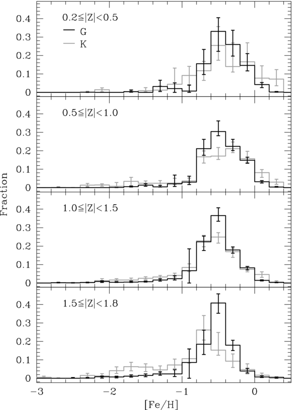
Figure 16. Weighted MDF over the overlap distance range for the G (black) and K (gray) dwarfs at a range of |Z|, where |Z| is the current distance from the plane in kpc. The uncertainty in each bin was determined from our bootstrap analysis over 500 iterations combined with additional measured uncertainties (Section 5.2). These distributions are listed in Tables 6 and 7.
Download figure:
Standard image High-resolution image6. DISCUSSION
6.1. The MDF for Different Spectral Types
Past work by Favata et al. (1997) found a distribution of nearby K-dwarf stars that was significantly more deficient in metal-poor stars than their G-dwarf sample. They conjectured that this result could originate from either a metallicity bias in their original catalog or metal-enhanced cool star formation. However, later work by Rocha-Pinto & Maciel (1998) found their K-dwarf sample in good agreement with their G dwarfs. Similarly, Kotoneva et al. (2002) found a much broader distribution of K dwarfs with respect to [Fe/H] than Favata et al. (1997). Likely, the narrow distribution of K dwarfs in Favata et al. (1997) was due to small sample size and a tendency to target brighter stars for spectroscopy.
We compare the MDF of the weighted SEGUE G and K dwarfs over the overlapping distance range in Figure 13. Our analysis confirms the work of Rocha-Pinto & Maciel (1998), which found the distribution of metallicity in G and K dwarfs in the solar neighborhood to be in good agreement. For the overlap region for the G and K dwarfs, i.e., between 1.59 and 1.84 kpc, both spectral types peak at around [Fe/H] of −0.5, consistent with the peak metallicity for the α-enhanced sample identified by Lee et al. (2011b). The peak agreement of the two spectral types implies that the chemical enrichment and star formation history for the G and K dwarfs are quite similar.
The MDFs with respect to |Z| of the two spectral types differ at the extremes of the metallicity distribution (Figure 16). For heights below 1 kpc, the K dwarfs have a larger population of metal-rich stars. As discussed in Section 4.6, our color criteria for G dwarfs will remove the most metal-rich stars with ages greater than 5 Gyr. Above 1 kpc, there are few stars at or above solar metallicity, so the discrepancy between the two spectral types is no longer noticeable.
When we examine the metal-poor end for the G- and K-dwarf samples at different |Z|, we find a discrepancy (Figure 17). For |Z| distances below 1.5 kpc, the fractional contributions of stars with [Fe/H] <−1.0 agree within 1σ (Figure 17). The percentage of stars below [Fe/H] of −1.0 is consistent for the two spectral types up to |Z| = 1.5 kpc. However, at |Z| greater than 1.5 kpc, the percentage of metal-poor ([Fe/H] <− 1.0) K dwarfs is significantly larger than the metal-poor G dwarfs. For |Z| > 1.5 kpc, the fraction of G dwarfs increases from ∼6% at smaller |Z| to 9+7−5%. The K-dwarf percentage increases significantly more, from around 15% for 0.2 ⩽|Z| < 1.5 kpc to 32+15−12% above |Z| of 1.5 kpc (see Tables 4–7). For smaller |Z|, the median metallicities for both G and K dwarfs agree to within 0.04 dex. For the highest |Z| bin, the median metallicity for the G dwarfs is −0.55, whereas the K-dwarf median [Fe/H] is −0.74, much more metal-poor.
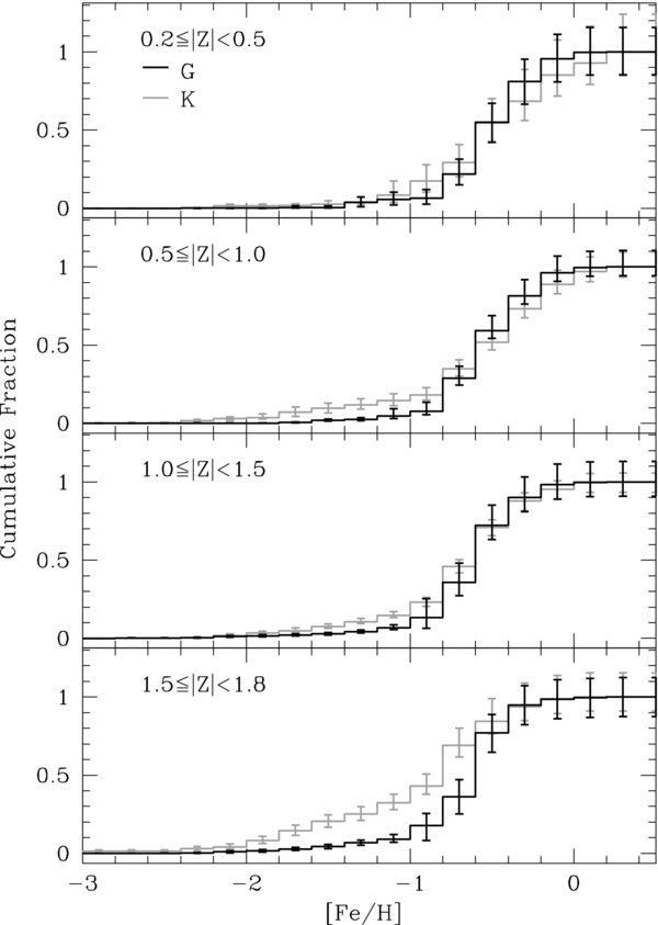
Figure 17. Cumulative-weighted MDF over the overlap distance range for the G (black) and K (gray) dwarfs at a range of |Z|, where |Z| is the current distance from the plane in kpc. We combine the error bars for each individual metallicity bin (from our bootstrap and Monte Carlo analysis) together in quadrature to determine the uncertainty for each cumulative bin. Above |Z| of 0.5 kpc, the K dwarfs show a more prominent metal-poor tail than the G dwarfs. Note that the fractions of the G- and K-dwarf sample below [Fe/H] of −1.0 are consistent until |Z| ⩾ 1.5 kpc.
Download figure:
Standard image High-resolution imageTable 4. The Metallicity Distribution Functions of G Dwarfs over Different Ranges of |Z| for 1.59 ⩽ d ⩽ 2.29 kpc
| [Fe/H] | 0.0 ⩽|Z| < 0.5 kpc | 0.5 ⩽|Z| < 1.0 kpc | 1.0 ⩽|Z| < 1.5 kpc | 1.5 ⩽|Z| < 2.5 kpc | ||||||||||||
|---|---|---|---|---|---|---|---|---|---|---|---|---|---|---|---|---|
| Raw | Weighted | Raw | Weighted | Raw | Weighted | Raw | Weighted | |||||||||
| +0 | +0 | +0 | +0 | +0 | +0 | +0 | +0 | |||||||||
| −3.3 | 0 | 0 | 0 | 0 | 0 | 0 | 0 | 0 | ||||||||
| −0 | −0 | −0 | −0 | −0 | −0 | −0 | −0 | |||||||||
| +0 | +0 | +1 | +1 | +0 | +0 | +1 | +0 | |||||||||
| −3.1 | 0 | 0 | 1 | 1 | 0 | 0 | 1 | 0 | ||||||||
| −0 | −0 | −1 | −1 | −0 | −0 | −1 | −0 | |||||||||
| +0 | +0 | +1 | +13 | +0 | +0 | +1 | +2 | |||||||||
| −2.9 | 0 | 0 | 1 | 12 | 0 | 0 | 2 | 3 | ||||||||
| −0 | −0 | −1 | −13 | −0 | −0 | −2 | −2 | |||||||||
| +0 | +0 | +1 | +12 | +3 | +7 | +2 | +5 | |||||||||
| −2.7 | 0 | 0 | 2 | 13 | 4 | 9 | 2 | 4 | ||||||||
| −0 | −0 | −1 | −9 | −2 | −6 | −1 | −3 | |||||||||
| +1 | +0 | +2 | +2 | +2 | +3 | +3 | +7 | |||||||||
| −2.5 | 1 | 0 | 2 | 2 | 3 | 3 | 3 | 3 | ||||||||
| −1 | −0 | −2 | −2 | −2 | −2 | −2 | −2 | |||||||||
| +1 | +4 | +3 | +24 | +3 | +7 | +5 | +5 | |||||||||
| −2.3 | 1 | 3 | 3 | 10 | 10 | 17 | 12 | 8 | ||||||||
| −1 | −2 | −2 | −6 | −4 | −7 | −4 | −4 | |||||||||
| +1 | +0 | +4 | +75 | +7 | +27 | +8 | +9 | |||||||||
| −2.1 | 1 | 0 | 7 | 103 | 20 | 58 | 31 | 29 | ||||||||
| −1 | −0 | −3 | −52 | −4 | −22 | −9 | −10 | |||||||||
| +0 | +0 | +4 | +6 | +9 | +20 | +10 | +11 | |||||||||
| −1.9 | 0 | 0 | 8 | 10 | 37 | 63 | 49 | 37 | ||||||||
| −0 | −0 | −3 | −4 | −9 | −19 | −13 | −11 | |||||||||
| +2 | +140 | +8 | +39 | +13 | +34 | +14 | +17 | |||||||||
| −1.7 | 3 | 146 | 31 | 88 | 52 | 98 | 52 | 55 | ||||||||
| −2 | −135 | −8 | −25 | −10 | −31 | −7 | −12 | |||||||||
| +3 | +135 | +12 | +139 | +17 | +30 | +18 | +18 | |||||||||
| −1.5 | 1 | 58 | 33 | 201 | 62 | 94 | 91 | 72 | ||||||||
| −1 | −50 | −5 | −48 | −8 | −18 | −17 | −16 | |||||||||
| +2 | +166 | +11 | +130 | +19 | +45 | +22 | +28 | |||||||||
| −1.3 | 2 | 121 | 32 | 170 | 99 | 196 | 143 | 126 | ||||||||
| −2 | −121 | −6 | −50 | −24 | −57 | −28 | −30 | |||||||||
| +3 | +267 | +28 | +226 | +30 | +63 | +69 | +38 | |||||||||
| −1.1 | 6 | 428 | 87 | 478 | 203 | 303 | 239 | 127 | ||||||||
| −5 | −389 | −13 | −89 | −37 | −59 | −41 | −24 | |||||||||
| +19 | +332 | +74 | +660 | +403 | +718 | +171 | +108 | |||||||||
| −0.9 | 7 | 115 | 121 | 1012 | 367 | 651 | 483 | 303 | ||||||||
| −5 | −91 | −26 | −257 | −31 | −72 | −136 | −85 | |||||||||
| +5 | +428 | +30 | +922 | +62 | +258 | +110 | +126 | |||||||||
| −0.7 | 25 | 1217 | 286 | 6443 | 638 | 2319 | 751 | 839 | ||||||||
| −7 | −359 | −25 | −741 | −67 | −284 | −57 | −68 | |||||||||
| +5 | +355 | +32 | +1142 | +44 | +271 | +35 | +118 | |||||||||
| −0.5 | 35 | 1984 | 358 | 9024 | 660 | 3784 | 497 | 1338 | ||||||||
| −7 | −464 | −16 | −496 | −42 | −297 | −24 | −68 | |||||||||
| +7 | +389 | +15 | +538 | +15 | +85 | +17 | +43 | |||||||||
| −0.3 | 40 | 1769 | 350 | 7346 | 421 | 1815 | 234 | 512 | ||||||||
| −6 | −277 | −24 | −668 | −32 | −175 | −16 | −38 | |||||||||
| +7 | +307 | +17 | +298 | +22 | +85 | +9 | +15 | |||||||||
| −0.1 | 40 | 1093 | 318 | 4012 | 258 | 746 | 104 | 152 | ||||||||
| −6 | −173 | −21 | −341 | −15 | −59 | −13 | −22 | |||||||||
| +5 | +68 | +12 | +90 | +12 | +19 | +8 | +8 | |||||||||
| 0.1 | 22 | 224 | 169 | 888 | 104 | 109 | 35 | 26 | ||||||||
| −5 | −66 | −18 | −151 | −14 | −17 | −7 | −6 | |||||||||
| +2 | +12 | +7 | +32 | +7 | +7 | +4 | +4 | |||||||||
| 0.3 | 9 | 40 | 52 | 88 | 32 | 30 | 9 | 8 | ||||||||
| −4 | −17 | −10 | −18 | −9 | −10 | −4 | −4 | |||||||||
| +0 | +0 | +1 | +1 | +0 | +0 | +0 | +0 | |||||||||
| 0.5 | 0 | 0 | 1 | 1 | 0 | 0 | 0 | 0 | ||||||||
| −0 | −0 | −1 | −1 | −0 | −0 | −0 | −0 | |||||||||
Notes. The G-dwarf raw and weighted metallicity distribution function for different ranges of |Z|. This is for the G-dwarf sample limited to distances between 1.59 and 2.29 kpc.
Download table as: ASCIITypeset image
Table 5. The Metallicity Distribution Functions of K Dwarfs over Different Ranges of |Z| for 1.18 ⩽ d ⩽ 1.84 kpc
| [Fe/H] | 0.0 ⩽|Z| < 0.5 kpc | 0.5 ⩽|Z| < 1.0 kpc | 1.0 ⩽|Z| < 1.5 kpc | 1.5 ⩽|Z| < 2.5 kpc | ||||||||||||
|---|---|---|---|---|---|---|---|---|---|---|---|---|---|---|---|---|
| Raw | Weighted | Raw | Weighted | Raw | Weighted | Raw | Weighted | |||||||||
| +0 | +0 | +1 | +6 | +0 | +0 | +0 | +0 | |||||||||
| −3.3 | 0 | 0 | 1 | 7 | 0 | 0 | 0 | 0 | ||||||||
| −0 | −0 | −1 | −7 | −0 | −0 | −0 | −0 | |||||||||
| +0 | +0 | +1 | +46 | +2 | +10 | +1 | +8 | |||||||||
| −3.1 | 0 | 0 | 1 | 6 | 3 | 9 | 2 | 10 | ||||||||
| −0 | −0 | −1 | −6 | −2 | −6 | −2 | −8 | |||||||||
| +1 | +10 | +0 | +0 | +2 | +7 | +2 | +7 | |||||||||
| −2.9 | 1 | 10 | 0 | 0 | 2 | 6 | 2 | 6 | ||||||||
| −1 | −10 | −0 | −0 | −1 | −4 | −1 | −5 | |||||||||
| +1 | +32 | +2 | +79 | +3 | +20 | +0 | +0 | |||||||||
| −2.7 | 1 | 21 | 3 | 21 | 12 | 16 | 0 | 0 | ||||||||
| −1 | −15 | −2 | −11 | −4 | −6 | −0 | −0 | |||||||||
| +1 | +5 | +2 | +18 | +5 | +11 | +0 | +0 | |||||||||
| −2.5 | 1 | 4 | 8 | 27 | 15 | 26 | 0 | 0 | ||||||||
| −1 | −3 | −4 | −14 | −4 | −9 | −0 | −0 | |||||||||
| +2 | +67 | +6 | +186 | +7 | +35 | +2 | +13 | |||||||||
| −2.3 | 2 | 21 | 21 | 406 | 23 | 61 | 4 | 19 | ||||||||
| −1 | −14 | −5 | −168 | −4 | −14 | −2 | −12 | |||||||||
| +3 | +125 | +6 | +162 | +10 | +73 | +4 | +15 | |||||||||
| −2.1 | 7 | 136 | 26 | 373 | 50 | 148 | 11 | 16 | ||||||||
| −3 | −75 | −5 | −128 | −7 | −29 | −4 | −6 | |||||||||
| +4 | +590 | +14 | +445 | +13 | +63 | +5 | +27 | |||||||||
| −1.9 | 7 | 442 | 51 | 423 | 74 | 234 | 16 | 51 | ||||||||
| −3 | −237 | −7 | −107 | −9 | −33 | −5 | −17 | |||||||||
| +4 | +77 | +11 | +643 | +15 | +90 | +6 | +30 | |||||||||
| −1.7 | 9 | 171 | 52 | 898 | 99 | 346 | 17 | 77 | ||||||||
| −3 | −61 | −7 | −448 | −13 | −57 | −4 | −26 | |||||||||
| +4 | +167 | +14 | +292 | +17 | +83 | +4 | +21 | |||||||||
| −1.5 | 12 | 337 | 81 | 1019 | 115 | 442 | 22 | 82 | ||||||||
| −4 | −149 | −12 | −230 | −13 | −71 | −7 | −34 | |||||||||
| +4 | +200 | +14 | +375 | +18 | +75 | +8 | +28 | |||||||||
| −1.3 | 12 | 155 | 72 | 1026 | 130 | 400 | 23 | 56 | ||||||||
| −4 | −65 | −9 | −264 | −16 | −67 | −5 | −16 | |||||||||
| +7 | +674 | +33 | +641 | +25 | +131 | +10 | +42 | |||||||||
| −1.1 | 27 | 1274 | 162 | 1078 | 204 | 630 | 33 | 91 | ||||||||
| −6 | −558 | −24 | −193 | −24 | −81 | −7 | −24 | |||||||||
| +12 | +400 | +32 | +371 | +44 | +164 | +19 | +57 | |||||||||
| −0.9 | 34 | 921 | 225 | 2050 | 374 | 1141 | 48 | 141 | ||||||||
| −6 | −305 | −25 | −310 | −44 | −152 | −6 | −31 | |||||||||
| +11 | +703 | +29 | +1004 | +27 | +286 | +10 | +104 | |||||||||
| −0.7 | 54 | 2520 | 321 | 6642 | 485 | 3591 | 48 | 336 | ||||||||
| −6 | −474 | −15 | −632 | −37 | −380 | −8 | −66 | |||||||||
| +15 | +1208 | +24 | +1062 | +17 | +212 | +9 | +126 | |||||||||
| −0.5 | 88 | 5272 | 410 | 8963 | 359 | 3509 | 27 | 190 | ||||||||
| −8 | −823 | −18 | −570 | −24 | −326 | −4 | −35 | |||||||||
| +15 | +1357 | +20 | +857 | +12 | +105 | +3 | +48 | |||||||||
| −0.3 | 100 | 5677 | 378 | 1.018 × 10⁴ | 202 | 2325 | 18 | 115 | ||||||||
| −8 | −503 | −19 | −674 | −17 | −321 | −6 | −42 | |||||||||
| +8 | +1049 | +17 | +1064 | +12 | +139 | +2 | +44 | |||||||||
| −0.1 | 77 | 5042 | 265 | 7486 | 121 | 1449 | 7 | 58 | ||||||||
| −10 | −745 | −17 | −528 | −11 | −203 | −3 | −28 | |||||||||
| +5 | +693 | +13 | +522 | +7 | +95 | +1 | +14 | |||||||||
| 0.1 | 33 | 2412 | 93 | 3096 | 47 | 574 | 3 | 20 | ||||||||
| −6 | −539 | −9 | −451 | −8 | −136 | −2 | −14 | |||||||||
| +4 | +513 | +4 | +415 | +6 | +64 | +0 | +0 | |||||||||
| 0.3 | 16 | 1631 | 55 | 1317 | 16 | 171 | 0 | 0 | ||||||||
| −4 | −468 | −13 | −323 | −4 | −60 | −0 | −0 | |||||||||
| +0 | +0 | +0 | +0 | +0 | +0 | +0 | +0 | |||||||||
| 0.5 | 0 | 0 | 0 | 0 | 0 | 0 | 0 | 0 | ||||||||
| −0 | −0 | −0 | −0 | −0 | −0 | −0 | −0 | |||||||||
Notes. The K-dwarf raw and weighted metallicity distribution function for different ranges of |Z|. This is for the distances between 1.18 and 1.84 kpc.
Download table as: ASCIITypeset image
Table 6. The Metallicity Distribution Functions of G Dwarfs over Different Ranges of |Z| for 1.59 ⩽ d ⩽ 1.84 kpc
| [Fe/H] | 0.0 ⩽|Z| < 0.5 kpc | 0.5 ⩽|Z| < 1.0 kpc | 1.0 ⩽|Z| < 1.5 kpc | 1.5 ⩽|Z| < 2.5 kpc | ||||||||||||
|---|---|---|---|---|---|---|---|---|---|---|---|---|---|---|---|---|
| Raw | Weighted | Raw | Weighted | Raw | Weighted | Raw | Weighted | |||||||||
| +0 | +0 | +0 | +0 | +0 | +0 | +0 | +0 | |||||||||
| −3.3 | 0 | 0 | 0 | 0 | 0 | 0 | 0 | 0 | ||||||||
| −0 | −0 | −0 | −0 | −0 | −0 | −0 | −0 | |||||||||
| +0 | +0 | +0 | +0 | +0 | +0 | +0 | +0 | |||||||||
| −3.1 | 0 | 0 | 0 | 0 | 0 | 0 | 0 | 0 | ||||||||
| −0 | −0 | −0 | −0 | −0 | −0 | −0 | −0 | |||||||||
| +0 | +0 | +0 | +0 | +0 | +0 | +0 | +0 | |||||||||
| −2.9 | 0 | 0 | 0 | 0 | 0 | 0 | 0 | 0 | ||||||||
| −0 | −0 | −0 | −0 | −0 | −0 | −0 | −0 | |||||||||
| +0 | +0 | +1 | +4 | +2 | +6 | +1 | +0 | |||||||||
| −2.7 | 0 | 0 | 1 | 4 | 2 | 6 | 1 | 0 | ||||||||
| −0 | −0 | −1 | −5 | −1 | −5 | −1 | −0 | |||||||||
| +1 | +0 | +2 | +3 | +1 | +3 | +2 | +2 | |||||||||
| −2.5 | 1 | 0 | 1 | 1 | 1 | 3 | 1 | 0 | ||||||||
| −1 | −0 | −1 | −1 | −1 | −3 | −1 | −0 | |||||||||
| +1 | +4 | +1 | +5 | +3 | +6 | +3 | +2 | |||||||||
| −2.3 | 1 | 3 | 2 | 3 | 6 | 9 | 3 | 0 | ||||||||
| −1 | −3 | −2 | −2 | −3 | −5 | −2 | −0 | |||||||||
| +1 | +0 | +0 | +0 | +5 | +17 | +3 | +3 | |||||||||
| −2.1 | 1 | 0 | 0 | 0 | 10 | 27 | 9 | 6 | ||||||||
| −1 | −0 | −0 | −0 | −3 | −16 | −7 | −5 | |||||||||
| +0 | +0 | +3 | +5 | +6 | +11 | +4 | +3 | |||||||||
| −1.9 | 0 | 0 | 6 | 6 | 12 | 14 | 7 | 5 | ||||||||
| −0 | −0 | −3 | −3 | −4 | −6 | −4 | −3 | |||||||||
| +2 | +36 | +5 | +26 | +13 | +18 | +7 | +5 | |||||||||
| −1.7 | 2 | 16 | 16 | 54 | 21 | 18 | 11 | 8 | ||||||||
| −2 | −15 | −7 | −27 | −7 | −7 | −5 | −3 | |||||||||
| +0 | +0 | +11 | +81 | +14 | +17 | +9 | +5 | |||||||||
| −1.5 | 0 | 0 | 19 | 130 | 24 | 24 | 22 | 11 | ||||||||
| −0 | −0 | −6 | −60 | −4 | −6 | −10 | −5 | |||||||||
| +1 | +132 | +15 | +65 | +10 | +23 | +13 | +8 | |||||||||
| −1.3 | 2 | 121 | 17 | 44 | 44 | 57 | 30 | 16 | ||||||||
| −2 | −98 | −5 | −16 | −12 | −20 | −9 | −5 | |||||||||
| +2 | +115 | +90 | +458 | +60 | +57 | +40 | +16 | |||||||||
| −1.1 | 1 | 79 | 41 | 208 | 97 | 86 | 44 | 16 | ||||||||
| −1 | −100 | −27 | −145 | −32 | −30 | −27 | −10 | |||||||||
| +13 | +127 | +51 | +317 | +345 | +431 | +97 | +51 | |||||||||
| −0.9 | 4 | 26 | 48 | 295 | 194 | 242 | 113 | 59 | ||||||||
| −4 | −33 | −19 | −127 | −196 | −248 | −121 | −63 | |||||||||
| +4 | +294 | +24 | +491 | +40 | +112 | +71 | +52 | |||||||||
| −0.7 | 14 | 599 | 131 | 2077 | 321 | 814 | 179 | 127 | ||||||||
| −5 | −229 | −16 | −361 | −63 | −172 | −54 | −39 | |||||||||
| +4 | +284 | +22 | +561 | +33 | +155 | +14 | +34 | |||||||||
| −0.5 | 21 | 1271 | 158 | 2986 | 308 | 1332 | 118 | 281 | ||||||||
| −6 | −416 | −10 | −230 | −19 | −113 | −15 | −38 | |||||||||
| +5 | +297 | +14 | +382 | +12 | +61 | +9 | +19 | |||||||||
| −0.3 | 20 | 997 | 151 | 2190 | 203 | 652 | 63 | 124 | ||||||||
| −4 | −244 | −11 | −214 | −18 | −65 | −8 | −20 | |||||||||
| +6 | +245 | +10 | +164 | +11 | +28 | +6 | +10 | |||||||||
| −0.1 | 23 | 562 | 159 | 1454 | 144 | 297 | 26 | 27 | ||||||||
| −4 | −115 | −18 | −162 | −16 | −40 | −6 | −7 | |||||||||
| +3 | +40 | +11 | +60 | +7 | +11 | +4 | +4 | |||||||||
| 0.1 | 17 | 163 | 70 | 315 | 56 | 52 | 9 | 5 | ||||||||
| −5 | −65 | −10 | −71 | −11 | −12 | −4 | −2 | |||||||||
| +2 | +12 | +5 | +22 | +6 | +5 | +1 | +2 | |||||||||
| 0.3 | 3 | 6 | 23 | 36 | 16 | 12 | 3 | 4 | ||||||||
| −2 | −3 | −5 | −10 | −5 | −4 | −3 | −3 | |||||||||
| +0 | +0 | +1 | +1 | +0 | +0 | +0 | +0 | |||||||||
| 0.5 | 0 | 0 | 1 | 1 | 0 | 0 | 0 | 0 | ||||||||
| −0 | −0 | −1 | −1 | −0 | −0 | −0 | −0 | |||||||||
Notes. The G-dwarf raw and weighted metallicity distribution function for different ranges of |Z|. This is for the distances between 1.59 and 1.84 kpc.
Download table as: ASCIITypeset image
Table 7. The Metallicity Distribution Functions of K Dwarfs over Different Ranges of |Z| for 1.59 ⩽ d ⩽ 1.84 kpc
| [Fe/H] | 0.0 ⩽|Z| < 0.5 kpc | 0.5 ⩽|Z| < 1.0 kpc | 1.0 ⩽|Z| < 1.5 kpc | 1.5 ⩽|Z| < 2.5 kpc | ||||||||||||
|---|---|---|---|---|---|---|---|---|---|---|---|---|---|---|---|---|
| Raw | Weighted | Raw | Weighted | Raw | Weighted | Raw | Weighted | |||||||||
| +0 | +0 | +0 | +0 | +0 | +0 | +0 | +0 | |||||||||
| −3.3 | 0 | 0 | 0 | 0 | 0 | 0 | 0 | 0 | ||||||||
| −0 | −0 | −0 | −0 | −0 | −0 | −0 | −0 | |||||||||
| +0 | +0 | +1 | +49 | +2 | +5 | +1 | +9 | |||||||||
| −3.1 | 0 | 0 | 1 | 6 | 1 | 1 | 2 | 10 | ||||||||
| −0 | −0 | −1 | −6 | −1 | −1 | −2 | −8 | |||||||||
| +0 | +0 | +0 | +0 | +0 | +0 | +2 | +7 | |||||||||
| −2.9 | 0 | 0 | 0 | 0 | 0 | 0 | 2 | 6 | ||||||||
| −0 | −0 | −0 | −0 | −0 | −0 | −1 | −5 | |||||||||
| +0 | +0 | +1 | +86 | +3 | +19 | +0 | +0 | |||||||||
| −2.7 | 0 | 0 | 2 | 17 | 1 | 1 | 0 | 0 | ||||||||
| −0 | −0 | −2 | −13 | −1 | −1 | −0 | −0 | |||||||||
| +0 | +0 | +1 | +13 | +2 | +8 | +0 | +0 | |||||||||
| −2.5 | 0 | 0 | 1 | 8 | 5 | 11 | 0 | 0 | ||||||||
| −0 | −0 | −1 | −7 | −3 | −6 | −0 | −0 | |||||||||
| +1 | +35 | +4 | +171 | +5 | +25 | +2 | +14 | |||||||||
| −2.3 | 1 | 3 | 8 | 267 | 7 | 14 | 4 | 19 | ||||||||
| −1 | −3 | −3 | −148 | −3 | −6 | −2 | −12 | |||||||||
| +1 | +73 | +3 | +130 | +6 | +70 | +4 | +14 | |||||||||
| −2.1 | 2 | 104 | 11 | 279 | 24 | 90 | 10 | 15 | ||||||||
| −2 | −82 | −4 | −134 | −6 | −26 | −4 | −6 | |||||||||
| +0 | +0 | +5 | +398 | +7 | +50 | +5 | +26 | |||||||||
| −1.9 | 0 | 0 | 18 | 142 | 32 | 106 | 15 | 50 | ||||||||
| −0 | −0 | −5 | −49 | −6 | −25 | −5 | −18 | |||||||||
| +1 | +33 | +5 | +420 | +9 | +76 | +5 | +29 | |||||||||
| −1.7 | 1 | 23 | 13 | 667 | 31 | 105 | 17 | 77 | ||||||||
| −1 | −19 | −4 | −473 | −6 | −25 | −4 | −27 | |||||||||
| +2 | +115 | +5 | +237 | +9 | +50 | +4 | +23 | |||||||||
| −1.5 | 2 | 65 | 31 | 456 | 46 | 175 | 21 | 74 | ||||||||
| −2 | −44 | −9 | −176 | −11 | −48 | −7 | −29 | |||||||||
| +2 | +165 | +5 | +271 | +8 | +50 | +8 | +27 | |||||||||
| −1.3 | 3 | 88 | 19 | 469 | 57 | 223 | 22 | 56 | ||||||||
| −2 | −65 | −5 | −183 | −11 | −56 | −5 | −16 | |||||||||
| +9 | +627 | +12 | +500 | +12 | +86 | +10 | +39 | |||||||||
| −1.1 | 5 | 316 | 51 | 489 | 78 | 275 | 31 | 89 | ||||||||
| −4 | −327 | −13 | −162 | −13 | −52 | −6 | −23 | |||||||||
| +4 | +355 | +14 | +280 | +29 | +129 | +21 | +66 | |||||||||
| −0.9 | 11 | 657 | 59 | 710 | 154 | 571 | 43 | 131 | ||||||||
| −5 | −390 | −14 | −188 | −38 | −153 | −5 | −29 | |||||||||
| +3 | +360 | +11 | +625 | +17 | +207 | +9 | +97 | |||||||||
| −0.7 | 10 | 844 | 98 | 3229 | 180 | 1547 | 45 | 322 | ||||||||
| −3 | −379 | −10 | −658 | −18 | −218 | −7 | −67 | |||||||||
| +6 | +737 | +15 | +901 | +10 | +161 | +9 | +119 | |||||||||
| −0.5 | 20 | 1826 | 115 | 3322 | 150 | 1688 | 26 | 188 | ||||||||
| −4 | −578 | −9 | −363 | −15 | −220 | −3 | −35 | |||||||||
| +7 | +920 | +10 | +703 | +8 | +127 | +3 | +47 | |||||||||
| −0.3 | 20 | 1003 | 118 | 4101 | 74 | 1150 | 18 | 115 | ||||||||
| −3 | −212 | −10 | −435 | −9 | −210 | −6 | −42 | |||||||||
| +5 | +739 | +10 | +784 | +9 | +112 | +2 | +38 | |||||||||
| −0.1 | 12 | 1192 | 75 | 3033 | 36 | 502 | 7 | 58 | ||||||||
| −3 | −355 | −8 | −373 | −5 | −93 | −3 | −30 | |||||||||
| +3 | +483 | +4 | +316 | +3 | +93 | +1 | +14 | |||||||||
| 0.1 | 7 | 554 | 30 | 1588 | 18 | 314 | 3 | 20 | ||||||||
| −3 | −238 | −7 | −499 | −5 | −108 | −2 | −15 | |||||||||
| +2 | +367 | +3 | +286 | +4 | +73 | +0 | +0 | |||||||||
| 0.3 | 4 | 516 | 11 | 590 | 1 | 9 | 0 | 0 | ||||||||
| −2 | −259 | −3 | −241 | −1 | −6 | −0 | −0 | |||||||||
| +0 | +0 | +0 | +0 | +0 | +0 | +0 | +0 | |||||||||
| 0.5 | 0 | 0 | 0 | 0 | 0 | 0 | 0 | 0 | ||||||||
| −0 | −0 | −0 | −0 | −0 | −0 | −0 | −0 | |||||||||
Notes. The K-dwarf raw and weighted metallicity distribution function for different ranges of |Z|. This is for the distances between 1.59 and 1.84 kpc.
Download table as: ASCIITypeset image
The origins of this discrepancy are currently unclear. The optimized version of the SSPP ensures that the [Fe/H] estimates for the G and K dwarfs are consistent with one another; there is no systematic offset in SSPP metallicity between the two spectral types of this size (Appendix A.2). One possible cause of the MDF differences at large |Z| is our assumed binarity fraction. If there is a larger probability of an undetected companion for K dwarfs than G dwarfs, we will be underestimating the distance to more K stars. This will cause more metal-poor stars to fall into the K-dwarf sample.
Examination of the G- and K-dwarf MDF at different heights above the Galactic plane reveals that the K dwarfs are more metal-rich at low heights and more metal-poor at large |Z|. This makes the total K-dwarf MDF appear broader than the G-dwarf MDF over the overlapping distance range. As the fraction below [Fe/H] of −1.0 from both spectral types is consistent within 2σ, we leave a more in-depth study of the metal-poor end of the G- and K-dwarf MDF for a future paper.
6.2. Extending the G-dwarf Problem
The original G-dwarf problem stemmed from the observational results that a simple closed box model of chemical evolution overpredicted the number of metal-poor stars. In the top row of Figure 18, we compare our total MDF of G and K dwarfs to a simple closed box model with instantaneous recycling, based on Pagel (1997). As expected, we find that our empirical distributions of both G and K dwarfs are deficient at the low-metallicity end when compared to these models, confirming that the G-dwarf problem persists in the large Galactic volume of our survey and to lower temperatures. For the total sample, the fraction of K stars with [Fe/H] less than −0.8 is ∼17+5−3%, whereas the model predicts 28%. Similarly, the model predicts that 27% of G dwarfs should have [Fe/H] <−0.8, but we observe ∼10+3−2%.
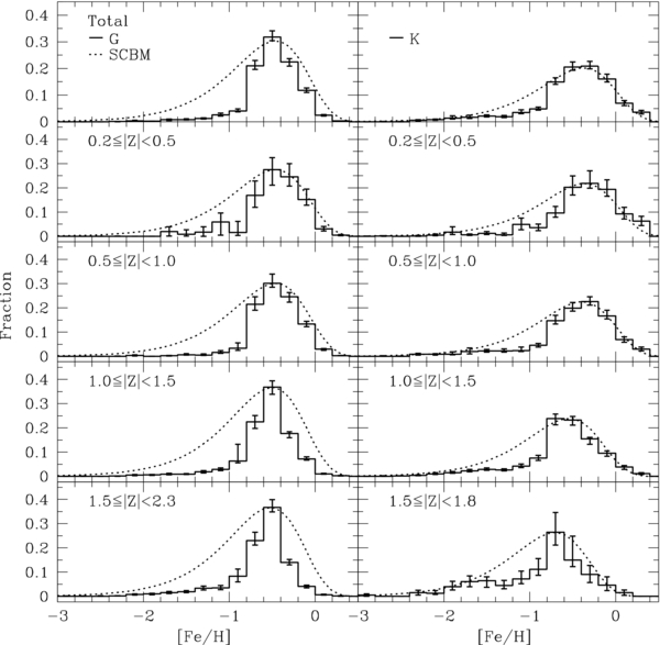
Figure 18. Comparison of the G- (left) and K-dwarf (right) sample in bins of |Z| with a simple closed box model (dotted line) assuming instantaneous recycling (Schmidt 1963). The total metallicity distribution for each spectral type over its associated distance range is shown in the top row. The size of the discrepancy between the observed distribution and the model at the metal-poor end is consistent for G and K dwarfs. The G- and K-dwarf problem is evident throughout the Milky Way disk.
Download figure:
Standard image High-resolution imageThe G-dwarf problem was originally reported for stars within the solar neighborhood. Using the SEGUE sample, we find that the discrepancy with the simple closed box model is evident throughout the disk (Figure 18). The discrepancies are on the order of 10%–20% between the observed distribution and the simple closed box model, enhanced at larger distances from the plane, and consistent between the spectral types.
6.3. Comparison of the G- and K-dwarf MDF with Previous Work
Our total MDF for G and K dwarfs covers a substantial portion of both the thin and thick in situ Milky Way disk. As a consequence, the peak metallicity for both spectral types is lower than previous analyses, such as RAVE (Siebert et al. 2011; Coşkunoğlu et al. 2012; Bilir et al. 2012) and GCS (Holmberg et al. 2007; Casagrande et al. 2011), which are dominated by thin-disk, more metal-rich stars. Similarly, the local MDFs for smaller samples, such as Rocha-Pinto & Maciel (1998) and Kotoneva et al. (2002), are more metal-rich than ours. These analyses have no stars in common with the SEGUE sample and probe a lower |Z| range. Although the lowest |Z| bin of G and K dwarfs ranges from 0.2 to 0.5 kpc, the median distance from the Galactic plane for these SEGUE stars is around 0.4 dex. Thus, our low-|Z| MDF is not directly comparable with local samples, and we defer this analysis to a later paper.
Allende Prieto et al. (2006) measure the MDF of G-dwarf stars, identified by effective temperature, between |Z| of 1 and 3 kpc. This volume of space is dominated by the thick disk. Allende Prieto et al. (2006) used the SDSS calibration star sample to examine the MDF between 1 and 3 kpc, a volume of space dominated by the thick disk. The size and homogeneity of the data enabled measurements of the change in the observed sample MDF with respect to distance from the plane. However, this sample pre-dated the SEGUE survey, and the calibration star selection introduced significant metallicity and evolutionary bias. The target selection of their sample causes the MDF of Allende Prieto et al. (2006) to drop off steeply above [Fe/H] of −0.4; it may also cause the MDF to peak at around [Fe/H] of −0.7, more metal-poor than our MDF above |Z| of 1 kpc.
Whereas the GCS, RAVE, and Allende Prieto et al. (2006) sample probe individual components of the disk, the photometric analyses of Ivezić et al. (2008) and Bond et al. (2010) examine a larger volume of space, from |Z| of 0.8 to 7 kpc. At heights below 2 kpc, their MDF is slightly more metal-poor than ours, by around 0.1–0.2 dex, perhaps due to inaccuracies in their photometric metallicity calibration. The contrasting MDFs of these different samples emphasize that the chemical structure of the disk varies significantly with respect to spatial location. Only with a uniform, extensive, spectroscopic sample such as SEGUE can we obtain accurate constraints on the chemistry of the disk as a whole.
6.3.1. Katz et al. (2011)
Past work by Katz et al. (2011) sought to constrain the vertical metallicity gradient of the thick disk alone. Their sample consists of approximately 400 stars along two lines of sight; they calculate atmospheric parameters using the ETOILE spectral-matching program. Utilizing a series of Besançon Galaxy models, they distinguish the thick-disk stars from the thin-disk population.
The MDF of the Katz et al. (2011) sample is slightly more metal-rich than our G- and K-dwarf sample at all |Z| (Figure 19). However, the two samples show general similarities to one another in structure and peak metallicity. Although the Katz et al. (2011) sample probes beyond the solar neighborhood, it is limited to only two lines of sight. Thus, it is promising for their analysis that we see general agreement in the metallicity distributions, but their limited sample size and volume make it difficult to measure the variation in the MDF at different locations in the disk.

Figure 19. Comparison of the SEGUE G- (left) and K-dwarf (right) MDFs with the distribution of Katz et al. (2011). The SEGUE samples are represented by the solid line and cover the spectral-type distance ranges. The Katz et al. (2011) distributions are plotted as the dashed lines. The MDF of the Katz et al. (2011) sample is typically more metal-rich than that of the G and K dwarfs.
Download figure:
Standard image High-resolution image6.3.2. Lee et al. (2011b)
Lee et al. (2011b) use the [α/Fe] ratios of the SEGUE G-dwarf stars to chemically separate the thin- and thick-disk components. They use a different sample than ours, extracting only stars specifically targeted as G dwarfs with S/N > 30, log g ⩾ 4.2, and distances within 3 kpc. We compare our G-dwarf metallicity distribution over the spectral distance range to the α-poor and α-enhanced metallicity distributions in Figure 20. In this figure, the two α-separated components are normalized by the total number of stars in the Lee et al. (2011b) sample. Farther away from the plane of the Galaxy, the α-rich component makes up a larger part of the sample, indicating that this α-rich population is an important contribution to our MDF far from the plane.
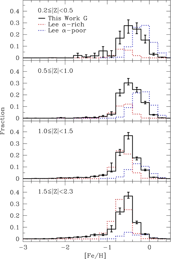
Figure 20. Comparison of the SEGUE G-dwarf MDF over the spectral-type distance range with that of Lee et al. (2011b). Their work is based on the SEGUE G-dwarf sample and divides their stars by [α/Fe]. Our SEGUE G dwarfs are plotted in black. The blue dashed line is the Lee et al. (2011b) α-poor sample, as a fraction of their entire sample of G dwarfs. The red dashed line is their α-enhanced distribution and normalized in the same manner. The Lee et al. (2011b) sample has not been corrected for observational biases; thus, the two distributions are skewed to be more metal-poor. At small |Z|, our corrected distributions appear to sample both the α components. The MDFs of our corrected distributions shift more metal-poor with increasing |Z|, better matching the α-enhanced sample.
Download figure:
Standard image High-resolution imageAt low heights above the plane, our observed MDFs contain a mix of the α-poor and α-rich samples from Lee et al. (2011b). At |Z| of 1.0 kpc, our MDF skews more metal-poor, matching the Lee et al. (2011b) α-rich sample better. This suggests that, at these heights, the G- and K-dwarf sample is dominated by the α-enhanced disk stars. Based on this comparison with the results of Lee et al. (2011b), our observed vertical variation in the MDF reflects the transition from a predominantly α-poor population at low |Z| to one dominated by α-rich stars at high |Z|, as well as a change in mean metallicity with distance from the plane.
6.4. Comparison with Galaxy Models
Models of chemical and dynamical evolution have evolved substantially since the simple closed box model of Schmidt (1963). Despite these improvements, models of Galaxy development remain hamstrung by the lack of extensive observational samples and are calibrated on samples from the local volume. Until SEGUE, there were few samples available to test and refine their predictions for the Milky Way properties far from the plane of the Galaxy. With our G- and K-dwarf MDFs, we can test existing Galaxy models and provide critical constraints on the metallicity structure with respect to location, to improve the model predictions and examine the star formation history of the disk far beyond the local volume. In particular, the range of |Z| heights makes the sample ideal for examining the transition between the thin and thick disk.
We compare our MDFs with predictions from two Galaxy models. Those of Schönrich & Binney (2009a, 2009b, SB) combine both chemical and dynamical evolution, whereas the TRILEGAL 1.4 model is based on empirical relationships. The models differ importantly in their modeling of the thick disk. While the TRILEGAL model treats the thick disk as a separate component of the Galaxy and allows different input parameters for its spatial distribution and local density, the SB models implement the radial migration of disk stars, forming a thick disk in the solar neighborhood via outward migration of older, inner disk stars. Thus, the SB model's metallicity distribution at high |Z| will be constrained by the chemistry of old, inner disk stars, while TRILEGAL's thick-disk metallicity distribution is fixed. We are also currently working on a comparison with the Besançon Galaxy model (Robin et al. 2003; K. J. Schlesinger et al. 2012, in preparation). We also have provided numerical tables of our MDFs (Tables 3–7) for comparison with future Galaxy models (e.g., Calura et al. 2012).
6.4.1. The Schönrich & Binney Galaxy Models
The models of Schönrich & Binney (2009a, 2009b) rely on assumed star formation laws, nucleosynthetic yields, and a Salpeter IMF (Salpeter 1955). These models base their star formation rate on the Kennicutt law (Kennicutt et al. 1998); Schönrich & Binney (2009a, 2009b) model the expected nucleosynthetic yields in conjunction with inflows, resulting in a predicted age–metallicity relationship, rather than building off an empirical version. In addition, these models include dynamical behavior, specifically, radial mixing, which alters the modeled chemical structure. Schönrich & Binney (2009b) compare the modeled vertical density structure to that of Jurić et al. (2008) and Ivezić et al. (2008), finding that the model accurately predicts the density structure of various Galaxy components. Finally, these models are built using the BaSTI isochrones (Pietrinferni et al. 2004), which they artificially widen to simulate the photometric errors of SDSS. Thus, the expected uncertainties derived from applying our techniques on these models should accurately reflect the photometric errors of the SEGUE sample. We do not factor the other uncertainties in the SEGUE sample, such as [Fe/H] and distance, into the SB models.
The SB model has been calibrated in [Fe/H] with the GCS (Nordström et al. 2004; Haywood 2008) and with updated parameters from Casagrande et al. (2011). Schönrich & Binney (2009a) have shown that their model accurately reflects the properties of stars in the solar neighborhood. They compare their model predictions to other observed samples, such as Fuhrmann (1998), Bensby et al. (2003), Reddy et al. (2006), and Haywood (2008), to constrain chemical parameters. Although many of these samples contain thick-disk stars, they are all limited to the solar neighborhood, which is thin-disk dominated. The GCS sample is typically within 200 pc (Casagrande et al. 2011). Similarly, the farthest distance probed by the Reddy et al. (2006) sample, which was selected based on Hipparcos data, is 150 pc. Thus, although the SB Galaxy model predicts the structure of the disk as a whole, it is only calibrated on the local volume.
6.4.2. The TRILEGAL Galaxy Models
Whereas the SB models simulate the disk's chemical and dynamical evolution, the TRILEGAL 1.4 models are more empirical in scope, utilizing a derived luminosity function, built from an assumed star formation rate, age–metallicity relation, and IMF. These parameters vary slightly for different components of the Galaxy.
The TRILEGAL 1.4 program allows us to simulate different lines of sight and assume a range of Galaxy parameters. We manufacture a TRILEGAL model for each SEGUE line of sight, using a limiting magnitude of 23.0 in r, no dust extinction, and no binary contamination over a circular 7 deg2 area of the sky. We specify an exponential thin disk with a two-step star formation rate. The thin disk is assigned a scale length of 2800 pc and a scale height that increases with stellar age, as described in Girardi et al. (2005). The assumed age–metallicity relationship for this component is based on the empirical determination from Rocha-Pinto et al. (2000) and includes α-enhancement at lower [M/H]. The thick disk is also modeled as an exponential, with a scale height of 800 pc and a scale length of 2800 pc. In contrast to the thin disk, a constant star formation rate and a Z of 0.008 ([Fe/H] = −0.7 for an α-rich population) and σ[M/H] of 0.1 dex (which is typically smaller than metallicity measurement errors) are assumed for the thick disk. In addition to the thin and thick disk, we specify an oblate spheroid halo and no central bulge. These properties are combined with the Padova evolutionary tracks to produce a derived luminosity function. Note that the TRILEGAL models predict the total metallicity, [M/H], rather than [Fe/H].
This model shows good agreement between the observed and predicted star counts when compared to various stellar catalogs, such as Two Micron All Sky Survey and Hipparcos (Girardi et al. 2005). There has been little chemical calibration of the TRILEGAL model.
6.4.3. Accuracy of Galaxy Models
We compare the G-dwarf metallicity distribution to the SB and TRILEGAL Galaxy models in Figures 21 and 22, respectively. For both models, we combine all of the SEGUE modeled lines of sight and extract all simulated stars that fulfill the color, magnitude, and distance criteria for our G-dwarf spectral type.
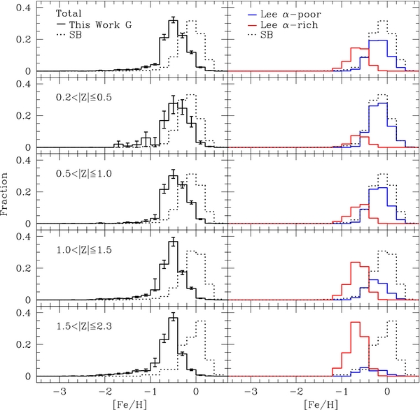
Figure 21. Comparison of the distribution of G-dwarf stars in the SEGUE sample (solid black) to that in the SB Galaxy models (dashed black) in the left column. Both sample and model are limited to distances between 1.59 and 2.29 kpc. The SB Galaxy model is significantly more metal-rich than the SEGUE G-dwarf sample. This discrepancy is also seen for the K-dwarf sample. On the right side, we compare the G-dwarf distribution in the model (dashed black) to the α-separated G-dwarf sample from Lee et al. (2011b). The sample with enhanced [α/Fe] is shown in red; that with low [α/Fe] is plotted in blue. For |Z| less than 1 kpc, the SB model is consistent with the α-poor distribution. Above 1 kpc, the model is more metal-rich than this component. The general agreement with solely the α-poor portion suggests that the SB models currently only recreate the chemistry of this portion of the Galaxy.
Download figure:
Standard image High-resolution image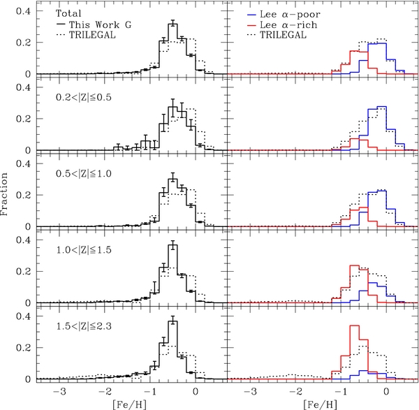
Figure 22. Same as Figure 21, except now for the TRILEGAL models, rather than those of Schönrich & Binney (2009a, 2009b). Note that TRILEGAL simulates total metallicity, [M/H], rather than [Fe/H]. We assume a simple linear relationship between [Fe/H] and [α/Fe] to adjust the model from [M/H] to [Fe/H]. This model predicts more metal-rich MDFs at all heights than our observed sample. Comparison with the α-separated samples of Lee et al. (2011b) suggests that at high |Z|, TRILEGAL does not adequately model the α-rich component. However, we can improve the agreement by adjusting the assumed [α/Fe]–[Fe/H] relationship. The comparison of SEGUE K dwarfs with the TRILEGAL model shows similar behavior.
Download figure:
Standard image High-resolution imageBoth of these models are calibrated to past analyses, which are typically limited to the local volume. Thus, we expect agreement between the model and SEGUE sample close to the plane of the Galaxy. However, Figures 21 and 22 indicate that, although there is substantial overlap in the range of [Fe/H], both models are more metal-rich and sharply peaked than our observed sample. The observed sample is broadened significantly by correlated errors in [Fe/H] and distance, in addition to general uncertainties in [Fe/H] (see Section 5.2 and Figure 7). The models do not simulate these uncertainties and thus exhibit a narrower MDF.
At higher distances from the plane, the metallicity discrepancy between the SB model and the SEGUE sample increases. Whereas the SEGUE distributions become more metal-poor with increasing |Z|, the models remain at an [Fe/H] of −0.1 for SB. In fact, the SB distributions become slightly more metal-rich at greater distances from the plane. We find similar discrepancies for the K-dwarf sample. We compare the SB modeled lines of sight with the α-separated stellar populations from Lee et al. (2011b) in Figure 21. The model agrees well with the α-poor distribution alone but is unable to accurately represent the α-rich component.
Rather than [Fe/H], the TRILEGAL model predicts [M/H], which includes contributions from [α/Fe]. The modeled [M/H] will thus be systematically higher than our [Fe/H] at large |Z|, where [α/Fe] is expected to be large. We model the relationship between [α/Fe] and [Fe/H] using a simple linear relationship based on the work of Lee et al. (2011b) and remove the expected [α/Fe] contribution from the [M/H] value of each simulated TRILEGAL star. We assume that stars of solar metallicity have [α/Fe] of 0. As [Fe/H] decreases, [α/Fe] increases to 0.20 at [Fe/H] = −0.5 and to 0.40 at [Fe/H] = −1.0. Without this correction, the distribution is similar to that of SB, where the model is systematically more metal-rich than the observations at all heights. When we account for [α/Fe], the match between our observed G-dwarf MDF and the model improves; however, TRILEGAL is still offset in [Fe/H], by around 0.1–0.2 dex, at all heights (Figure 22). We find that the model does not adequately simulate the structure of the α-rich population at large heights. In particular, from 1.5 to 2.3 kpc in |Z|, the TRILEGAL distribution is very similar to that of the Lee et al. (2011b) α-poor component. Note that we can improve the match between the simulation and observations by adjusting the contribution from [α/Fe].
The two models predict stars at large |Z| to be more metal-rich than we observe. The current inability of these Galaxy models, in particular the SB model, to predict the chemical structure of the disk points to the danger of assuming that the local volume reflects the properties over the span of the disk. Past analyses of the metallicity distribution, used to calibrate these Galaxy models, were limited to the solar neighborhood; they were dominated by thin-disk stars. While these samples contain thick-disk stars passing through the local volume, they may not provide a complete picture of the component's structure. There appears to be a significant disagreement between the picture of the disk structure from local kinematic samples and our in situ observations. Thus, our unbiased metallicity distributions of the SEGUE G and K dwarfs, and how they change with respect to R and |Z|, provide critical constraints for refining and improving Galaxy models, such that we gain a better understanding of the different chemical and dynamical processes occurring in the disk and no longer rely on local samples alone.
7. SUMMARY
In this work we examine the variation in [Fe/H] of the SEGUE G- and K-dwarf sample with respect to position in the Galaxy. These distributions allow us to better constrain the chemical and dynamical evolution processes in the disk. To ensure the accuracy of this sample, we optimize the SSPP to better handle low-temperature dwarfs and develop and test a procedure to account for target-selection biases in the SEGUE sample, using SDSS photometry for each individual line of sight. This technique corrects for the metal-poor bias in the spectroscopic sample and is critical for accurately constraining the metallicity structure of the Milky Way disk. For the first time, we can utilize an unbiased sample of both G and K dwarfs with accurate atmospheric parameters to examine the chemical structure over a large volume of the disk.
Using distances estimated with an isochrone-matching technique, accurate to ∼8% for metal-poor and ∼18% for metal-rich stars, we determine the MDFs of the G- and K-dwarf samples (Figure 13) and examine how the metallicity structure of the disk varies with respect to position and spectral type. Both the total MDFs and MDFs with respect to height above the plane of the Galaxy for the G- and K-dwarf samples are in good agreement with one another, implying that the two spectral types undergo similar chemodynamical evolution over the span of the disk. We compare both distributions to the simple closed box model, finding that the G-dwarf problem persists to both lower temperatures and is present throughout the volume of the Milky Way disk (Figure 18). This expands on previous work, such as Mould (1982), Favata et al. (1997), Flynn & Morell (1997), Rocha-Pinto & Maciel (1998), and Kotoneva et al. (2002), which examined the solar neighborhood. This is the first work where we can confirm that this discrepancy extends past the solar neighborhood with a large and unbiased stellar sample of two cool spectral types. In particular, all previous analyses of K dwarfs were much more limited in sample size and volume.
Analyses of the local volume find that the thin and thick disk are distinct with respect to [α/Fe]. As it is less likely than kinematics to change significantly over time, stellar chemistry is a useful diagnostic to disentangle the two components. Our analysis of the G- and K-dwarf MDF finds that both spectral types have more metal-poor stars as |Z| increases (Figure 16 and Tables 4–7), implying similar star formation histories. Comparison with the [α/Fe] analysis of Lee et al. (2011b) suggests that our vertical metallicity structure represents the transition from a population composed largely of α-poor stars at low |Z| to predominantly α-rich stars at high |Z|. This change with respect to |Z| is not predicted by the SB or TRILEGAL Galaxy models. Both are more metal-rich than our observed distribution. In particular, the SB model appears to simulate only the α-poor component of the Galaxy, suggesting that there are discrepancies with the picture of the extended disk presented by local samples and our own in situ observations. Thus, our observed MDFs provide a valuable constraint on future Galaxy formation and evolution models and strongly warn of the dangers of using existing models to predict behavior far from the local volume.
We thank J. Cheng and the anonymous referee for their valuable input on this work. K.S. and J.A.J acknowledge support from NSF grants AST-0807997 and AST-0607482. C.R. acknowledges support from the David and Lucille Packard Foundation. H.L.M. acknowledges support from AST-1009886. Y.S.L and T.C.B. acknowledge partial support from grant PHY 08-22648: Physics Frontiers Center/Joint Institute for Nuclear Astrophysics (JINA), awarded by the U.S. National Science Foundation.
Funding for SDSS-III has been provided by the Alfred P. Sloan Foundation, the Participating Institutions, the National Science Foundation, and the U.S. Department of Energy Office of Science. The SDSS-III Web site is http://www.sdss3.org/.
SDSS-III is managed by the Astrophysical Research Consortium for the Participating Institutions of the SDSS-III Collaboration including the University of Arizona, the Brazilian Participation Group, Brookhaven National Laboratory, University of Cambridge, University of Florida, the French Participation Group, the German Participation Group, the Instituto de Astrofisica de Canarias, the Michigan State/Notre Dame/JINA Participation Group, Johns Hopkins University, Lawrence Berkeley National Laboratory, Max Planck Institute for Astrophysics, New Mexico State University, New York University, Ohio State University, Pennsylvania State University, University of Portsmouth, Princeton University, the Spanish Participation Group, University of Tokyo, University of Utah, Vanderbilt University, University of Virginia, University of Washington, and Yale University.
APPENDIX A: OPTIMIZING THE SSPP FOR COOL DWARF STARS
The SSPP analyzes a wide range of spectral types, and not all of the techniques employed are appropriate for cool dwarfs. To ensure that the SSPP provides accurate atmospheric parameters for G and K dwarfs, we have developed an optimized version of the SSPP, carefully selecting, and occasionally adjusting, the log g and [Fe/H] techniques used in the analysis.
A.1. Surface-gravity Determinations
The SSPP uses 10 methods to estimate surface gravities for stars, each appropriate for a different range in (g − r)0 (Lee et al. 2008a). Although all of the techniques cover the range of (g − r)0 for G and K dwarfs, they are not all similarly accurate. As shown in Figure 23, the CaI2 and MgH indicators have large tails that extend to low values of log g not seen for other indicators. Comparison between log g estimates from Kepler and those from the SSPP indicates that the CaI2 and MgH techniques return systematically low surface gravities. To confirm this, we tested the different surface-gravity indicators on synthetic spectra (see Section 4.3 for more information); while the majority of the methods accurately reported the input log g, both CaI2 and MgH exhibited false low surface-gravity tails. Examination of the SSPP revealed that the implementation of these two techniques was flawed; both CaI2 and MgH utilized an inaccurate conversion between (g − r) and (B − V). Furthermore, we found that the relationship implemented in the SSPP for these techniques was an outdated version, different than that reported in Morrison et al. (2003). In addition to removing CaI2 and MgH, we also eliminate the log g estimate using the Wilhelm, Beers, and Gray (WBG) technique (Wilhelm et al. 1999). As it was designed for evolved stars, this indicator rarely works well for the G- and K-dwarf sample.
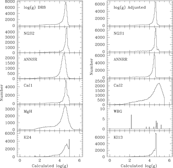
Figure 23. Surface gravities calculated using different methods in the SSPP for our sample of G and K dwarfs (see Lee et al. 2008a, 2008b for a description of methods). The original adopted log g distribution is in the top left. All of the distributions have a tail extending to log g values indicative of giants. However, this tail is significantly more pronounced for the CaI2 and MgH methods. Additionally, the width of the peaks for these two methods is larger than that of the others, making their estimate of log g generally more uncertain. The WBG method is, in general, unable to calculate a surface gravity for our targets. When the CaI2, MgH, and WBG techniques are removed, the low log g tail is diminished, and the peak of the distribution is narrower. This corrected log g is shown at the top right.
Download figure:
Standard image High-resolution imageUsing the CaI2, MgH, and WBG to determine log g will shift the calculated values lower, potentially eliminating some dwarfs from our sample by making their surface gravities indicative of evolved stars. For our targets, we use log g values that do not take these three methods into account. This tightens the distribution of surface gravities, diminishing the population that artificially lies in the low-valued tail (see Figure 23). On average, removing CaI2, MgH, and WBG increases the surface gravities from DR8 by less than 0.1 dex (see Figure 24).
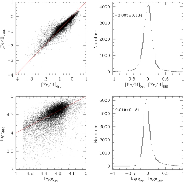
Figure 24. Comparison of the atmospheric parameters determined by the optimized version of the SSPP with those from DR8. The left column directly compares the values, with the optimized version on the x-axis and the DR8 on the y. The red line shows a one-to-one correlation. The right column shows the distribution of the difference between the two values for each parameter, with the mean and standard deviation of the difference noted in the top left corner. The top row is for [Fe/H] and bottom for log g.
Download figure:
Standard image High-resolution imageA.2. [Fe/H] Determinations
As with the surface-gravity estimates, not all of the metallicity-estimation techniques available in the SSPP are accurate for G and K dwarfs. For example, the CaIIK2 and WBG distributions are erratic and spiky (Figure 25). Other techniques, such as CaIIK3, ACF, ANNSR, and CaIIT, are limited in the metallicity range they cover, only reaching as high as solar metallicity. This limit will bias their measurements toward lower metallicities. We exclude these six techniques from our [Fe/H] determinations.
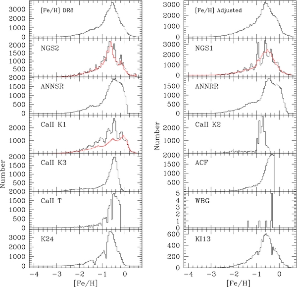
Figure 25. Metallicities calculated using different methods in the SSPP for our G- and K-dwarf sample. The original adopted [Fe/H] value is on the top left, with the adjusted distribution on the top right. For the different methods used in our optimized version of the SSPP, we plot the original distribution for the sample in black and the modified version in red. Note that for many methods, such as NGS1 and CaIIK1, the modified distribution is much smoother. We have also eliminated a number of methods as they either are not applicable for our sample or do not cover the appropriate metallicity range.
Download figure:
Standard image High-resolution image
Finally, there are other methods in the SSPP that appear to have well-behaved distributions in [Fe/H] but are inappropriate for our sample. Two of the Kurucz-model-based methods (KI13, K24) are designed for stars with temperatures greater than 5000 K; there are numerous K dwarfs for which this method is not accurate. The ANNRR method is also problematic; this neural-network technique is based on outdated parameters determined by the SSPP for DR7 (Abazajian et al. 2009). Thus, our [Fe/H] estimates are based solely on NGS2, NGS1, and CaIIK1.
Although these three remaining methods cover the appropriate range of parameter space, they still require adjustment. In particular, all three show artificial peaks. These methods utilize a χ2 minimization technique in Teff, log g, and [Fe/H] to match target spectra with various synthetic grids. These grids cover a fairly narrow range of parameter space, resulting in the sharply peaked structure. By modifying the χ2 interpolation method in parameter space from the [Fe/H] values reported in DR8 (Aihara et al. 2011), these peaks are smoothed, providing a more realistic distribution in [Fe/H]. Figure 24 indicates that, on average, these modifications have very little effect on the estimated [Fe/H]. These changes will be detailed in the upcoming SEGUE DR9 paper and are outside the scope of this work.
APPENDIX B: UNCERTAINTIES IN CALCULATED DISTANCES
B.1. Photometry
The photometric uncertainty of SDSS targets is typically 2%–3% for each filter. Using the TRILEGAL simulations along SEGUE lines of sight, we simulate the photometric uncertainties in SDSS based on a Gaussian distribution. These changes factor into distance uncertainties twice: first, when we match each target to an isochrone in (g − r)0, and second, when we calculate the distance in each individual filter. The change in distance with respect to photometric uncertainty is typically less than 6% over the entire metallicity range.
B.2. [Fe/H]
There are two main components of uncertainty in the SSPP [Fe/H] estimates. First, there is the error that reflects the variation from the different techniques used by the SSPP to estimate [Fe/H]. This uncertainty from the three methods we utilize has a mean value of 0.07 ± 0.06 dex. Second is the uncertainty determined by comparing with stars of known metallicity, from clusters and high-resolution observations. This uncertainty varies with respect to S/N, ranging from 0.24 dex for S/N of 50 to 0.45 dex for S/N of 10 (Lee et al. 2008a).
For each SEGUE line of sight, we examine how the S/N varies with respect to magnitude, simulating the relationship for the associated TRILEGAL model. Based on the assigned S/N, we estimate the expected [Fe/H] uncertainty, combining it in quadrature with a simulation of the pipeline [Fe/H] variation, convolved with a Gaussian. We then compare the original distances calculated for the TRILEGAL stars to those using [Fe/H] values adjusted for the simulated uncertainty. Changes in [Fe/H] have a larger effect on distance estimates for metal-rich stars ([Fe/H] >−1.0); these dominate the uncertainty with a distance error of 15%, whereas more metal-poor stars have an error of around 4%.
B.3. [α/Fe]
An et al. (2009) assign each YREC isochrone a specific [α/Fe] value based on its [Fe/H]. These values may not align with the [α/Fe] of the individual target, which will change the distance estimates, especially for the metal-rich regime where small changes in chemistry significantly change the isochrone. Lee et al. (2011a) found that for an S/N > 20, the SSPP can determine [α/Fe] with an uncertainty of approximately 0.1 dex. At lower S/N, the uncertainty increases to 0.2 dex. To estimate the change in estimated distance associated with a 0.2 dex uncertainty in [α/Fe], we compare the magnitudes of the Dartmouth isochrones at each value of [Fe/H] with [α/Fe] of 0 to those with [α/Fe] of +0.2 and −0.2. We must use the Dartmouth isochrones to estimate this effect, as the YREC isochrones do not model a range of [α/Fe] for each [Fe/H]. We simulate the change in Dartmouth ugriz at each [Fe/H] from a change in [α/Fe]; similar to the distance uncertainties from [Fe/H], the change in distance is larger, approximately 10%, at the metal-rich end. Below [Fe/H] of −1.0, the σd([α/Fe]) is approximately zero.
B.4. Isochrone Choice
Each individual isochrone set will yield slightly different ugriz values at the same (g − r), resulting in systematic differences in distance with respect to one another. The various assumptions integrated into each of these different isochrone sets means that for each (g − r) color, there is a range of appropriate r magnitude about the YREC value (Gallart et al. 2005). The difference between isochrone sets is more extreme at the metal-rich end, making the uncertainty due to isochrone choice larger than for metal-poor stars.
Distances calculated using YREC isochrones tend to be smaller than those calculated via Dartmouth isochrones by around 6% for stars with [Fe/H] ⩾−0.5; below this, the offset is around 3%. In contrast, both the BaSTI (Cassisi et al. 2006) and Padova (Girardi et al. 2004) isochrone sets will measure distances smaller than those from the YREC isochrones, approximately 8% for [Fe/H] ⩾ 0. For more metal-poor stars, the differences between BaSTI and YREC are around 1%.
Changing which isochrone set we use will induce a systematic change in our estimated distances. However, when we consider the many different isochrones, choosing a particular set can make our distances smaller or larger. Thus, we treat isochrone choice as a random uncertainty of approximately 7% for high-metallicity stars ([Fe/H] ⩾−0.5) and 3% for low-metallicity stars.
B.5. Age
To calculate distances, we assume that all stars have an age of 10 Gyr and compare them to isochrones of the same age. However, the actual ages of these stars are unknown. In particular, the most metal-rich stars are likely to be significantly younger than this value, causing us to systematically overestimate the distances to these stars.
To estimate the uncertainty from age, we utilize the modeled lines of sight from the SB Galaxy models. These models simulate a wide range of ages, from 2.5 to 11.5 Gyr using an age–metallicity relationship built off of expected nucleosynthetic yields (Section 6.4.1). In contrast, the TRILEGAL Galaxy model assumes an age–metallicity relationship from Rocha-Pinto et al. (2000) and contains stars from only 7 to 9 Gyr in age. For each modeled line of sight, we calculate the distances for simulated G and K dwarfs using 10 Gyr YREC isochrones. We then calculate the distances for the same sample using YREC isochrones that match the target in age, examining the differences between the two values. For the youngest stars, from 2.5 to 5 Gyr, using 10 Gyr isochrones creates a systematic 3% overestimate of distances. This value decreases as the ages of the stars increase. With respect to metallicity, this means that the metal-rich stars, with [Fe/H] >−0.4, will be systematically offset in distance from 1% to 3%. More metal-poor stars are unaffected. As all of our targets are on the main sequence, it is not surprising that we see little effect with respect to age assumptions; at this point in stellar evolution, isochrones of a given metallicity overlap quite closely.
B.6. Binarity
An undetected companion will make an individual target appear brighter and redder, causing us to underestimate the distance to the primary star. We simulate a population of binaries, using techniques described in Schlesinger et al. (2010), to examine how much undetected binarity will affect our distance calculations. We model a population of binaries, using a Chabrier IMF (Chabrier 2003) for both the primary and secondary stars, and determine the change in each ugriz filter with an undetected companion over a range of metallicity. We then match up each star in the TRILEGAL modeled lines of sight with these ugriz changes, comparing their original YREC distances to those estimated with the companion present. Binarity will typically lead to a systematic distance offset of 5%. Metal-poor stars ([Fe/H] <−1.0) have a slightly larger change in distance, around 7%–8%, whereas more metal-rich stars are around 4%. Although small changes in magnitude have a larger effect on distance estimates for metal-rich stars, the changes in magnitude from binarity are larger for metal-poor stars, such that the change in distance is slightly larger. As approximately 65% of all G and K stars are in binaries (Duquennoy & Mayor 1991), this results in a systematic offset to smaller distances of around 3%.
In addition to affecting photometry, undetected pairs can also alter our distance measurements via changes in the metallicity determination. The expected [Fe/H] uncertainty at an S/N of 25 is ±0.30 dex. Schlesinger et al. (2010) find that around 95% of all pairs will have a shift in [Fe/H] less than 0.15 dex. Thus, distance uncertainties stemming from a secondary's effect on [Fe/H] determinations are well within the error expected from the SSPP [Fe/H] determination, and we do not take them into account separately.
B.7. Summary of Random and Systematic Uncertainties in Distance
We have explored the different uncertainties that factor into our distance calculations using simulated lines of sight from TRILEGAL and SB Galaxy models. The random uncertainty in distance stems from photometry, [Fe/H] determinations, and [α/Fe] estimates. Photometry contributes a 6% uncertainty over the entire metallicity range; the chemistry of a star, however, causes a different amount of uncertainty for metal-rich and metal-poor stars. Metal-rich stars will have a change in distance of 16% from [Fe/H] and 10% from [α/Fe] uncertainty. At the metal-poor end, these values are smaller, around 4% from [Fe/H] and 0% from [α/Fe] uncertainty. In addition, we could use a number of different isochrones to estimate our distances, adding an additional random uncertainty in distance of 10% for metal-rich and 3% for metal-poor stars. Combining these in quadrature, we estimate our random distance uncertainty ranging from 15%–18% for [Fe/H] ⩾−1.0 to 8% for stars with [Fe/H] below −2.0 (Figure 3).
Our distance estimates also suffer from systematic uncertainties from age assumptions and binary contamination. While the distance uncertainties from age assumptions vary with metallicity, from 0% to 3% from the metal-poor to metal-rich end, binarity results in a more consistent offset of around 5% over the full [Fe/H] range.
B.8. Comparison with Ivezić et al. (2008) Photometric Parallax
Ivezić et al. (2008) develop a photometric parallax relationship that takes into account metallicity, building on the work by Jurić et al. (2008). The shape of the photometric relationship is based on SDSS observations of five globular clusters: M2, M3, M5, M13, and M15. These clusters range from 7 to 12 kpc in distance and −1.2 to −2.1 in [Fe/H] (Harris 1996). Using clusters from VandenBerg & Clem (2003), which range from −2.5 to +0.12 in [Fe/H], they then constrain the extent of magnitude shifts for different metallicities. Combining the equations determined for different ranges in (g − i), their final relationship is as follows:


Ivezić et al. (2008) specify that these equations are valid for dwarfs with 0.2 < (g − i) < 4.0. Less than 1% of G and K dwarfs fall outside of this color range. They expect uncertainties of around 5% and 10%–15% from systematic and random errors, respectively (Bond et al. 2010).
We compare our YREC isochrone distances to those calculated using photometric parallax, finding an offset of approximately 8%, with YREC distances typically smaller. This result is due to an ∼0.2 mag offset between the YREC isochrones and photometric metallicity relations. This offset varies with respect to metallicity: for [Fe/H] > 0, the change in distance is around 6%, whereas for [Fe/H] between −1.5 and −2.0, the change is minimal. Finally, for the most metal-poor stars ([Fe/H] <−2.0), the photometric parallax distances are actually smaller than those determined using YREC isochrones, by around 7%. To ensure that our distance method does not significantly change our results, we have also calculated the MDFs using photometric parallax distances instead of those from YREC. There are only slight changes, all of which are well within the expected bootstrap uncertainties for the distributions and gradients.
Footnotes
- 18
The likely existence of a second stellar component close to the Galactic plane was previously noted by Yoshii (1982), who referred to it as a halo component, even though its inferred density was 10 times that of the local halo. The Yoshii (1982) normalization relative to the local thin disk (0.01–0.02) and scale height (∼2 kpc) were commensurate with the values later determined by Gilmore & Reid (1983, 0.02 and 1.5 kpc, respectively). See also Yoshii et al. (1987).
- 19
Throughout the rest of this work, we will refer to plug plates simply as plates.
- 20
We find that these color cuts are equivalent to a spectral type of G5 or G6 for G dwarfs and G7 through K2 for K dwarfs (Johnson 1963).
- 21
The surface-gravity limit for these models is slightly higher than that applied to our sample, as these models are based on Padova isochrones (Girardi et al. 2004), which have the main-sequence turnoff at log g ≈ 4.2, whereas YREC isochrones place it at 4.1.
- 22
These reddening values were extracted from the DR7 table PhotoObjAll.
- 23
The photometric information is from the PhotoObjAll database in DR7.