


ABSTRACT
Secondary anisotropies in the cosmic microwave background are a treasure-trove of cosmological information. Interpreting current experiments probing them are limited by theoretical uncertainties rather than by measurement errors. Here we focus on the secondary anisotropies resulting from the thermal Sunyaev–Zel'dovich (tSZ) effect; the amplitude of which depends critically on the average thermal pressure profile of galaxy groups and clusters. To this end, we use a suite of hydrodynamical TreePM-SPH simulations that include radiative cooling, star formation, supernova feedback, and energetic feedback from active galactic nuclei. We examine in detail how the pressure profile depends on cluster radius, mass, and redshift and provide an empirical fitting function. We employ three different approaches for calculating the tSZ power spectrum: an analytical approach that uses our pressure profile fit, a semianalytical method of pasting our pressure fit onto simulated clusters, and a direct numerical integration of our simulated volumes. We demonstrate that the detailed structure of the intracluster medium and cosmic web affect the tSZ power spectrum. In particular, the substructure and asphericity of clusters increase the tSZ power spectrum by 10%–20% at ℓ ∼ 2000–8000, with most of the additional power being contributed by substructures. The contributions to the power spectrum from radii larger than R500 is ∼20% at ℓ = 3000, thus clusters interiors (r < R500) dominate the power spectrum amplitude at these angular scales.
Export citation and abstract BibTeX RIS
1. INTRODUCTION
As cosmic microwave background (CMB) photons travel through the diffuse hot gas comprising the bulk of baryons in galaxy clusters, a fraction of them are upscattered by the gas in a process called the thermal Sunyaev–Zel'dovich (tSZ) effect (Sunyaev & Zeldovich 1970). This scattering produces a unique spectral signature in the CMB, with a decrement in thermodynamic temperature below ν ∼ 220 GHz, and an excess above. The tSZ effect is typically seen on arcminute scales and is referred to as a secondary anisotropy, as it originates between us and the surface of last scattering, unlike the primary CMB anisotropies. In the non-relativistic limit, the tSZ is directly proportional to the integrated electron pressure along the line of sight. It typically traces out the spatial distribution of clusters and groups, since the hot intracluster medium (ICM) dominates the line-of-sight pressure integral. Thus, the tSZ provides an excellent tool to examine the bulk of cluster baryons. Found at the intersections of filaments in the cosmic web (Bond et al. 1996), clusters form at sites of constructive interference of long waves in the primordial density fluctuations, the coherent peak patches (Bardeen et al. 1986; Bond & Myers 1996). Clusters are sign posts for the growth of structure in the universe and are a potentially powerful tool for probing underlying cosmological parameters, such as w, the dark energy pressure-to-density ratio.
The angular power spectrum of the tSZ effect is extremely sensitive to cosmological parameters like σ8, the root mean square (rms) amplitude of the (linearized) density fluctuations on 8 h−1 Mpc scales. In fact, the amplitude of the tSZ power spectrum scales at least as steeply as the seventh power of σ8 (Bond et al. 2002; Komatsu & Seljak 2002; Bond et al. 2005; Trac et al. 2011) and improving the constraints on σ8 will aid in breaking the degeneracies found between σ8 and w when using only primary CMB constraints. An advantage of using the tSZ angular power spectrum over counting clusters is that no explicit measurement of cluster masses is required. Also, lower mass, and therefore fainter, clusters that may not be significantly detected as individual objects in CMB maps contribute to this statistical signal. However, disadvantages of using the tSZ angular power spectrum include potential contamination from point sources and that no redshift information from the clusters is used.
Previous observations by the Berkeley–Illinois–Maryland Association (Dawson et al. 2006), the Atacama Path-finding Experiment (Reichardt et al. 2009b), the Quest at DASI (Friedman et al. 2009), Arc-minute Cosmology Bolometer Array Receiver (Reichardt et al. 2009a), and the Cosmic Background Imager (Sievers et al. 2009) all measured excess power above that expected from primary anisotropies, which have been attributed to some combination of the tSZ effect and point-source contamination. The measurements from these experiments provided upper limits to the tSZ power spectrum amplitude. More recently, the Atacama Cosmology Telescope (ACT; Fowler et al. 2010; Dunkley et al. 2010) and the South Pole Telescope (SPT; Lueker et al. 2010; Shirokoff et al. 2010; Keisler et al. 2011) have detected the SZ effect in the CMB power spectrum.6 The results from ACT and SPT emphasize that the "sweet spot" for measuring the tSZ signal is between ℓ ∼ 2000 and 4000. Silk damping (Silk 1968) suppresses the power of primary anisotropies so that their contributions to the power spectrum are much smaller than the tSZ contribution at even higher ℓ. At these scales there are important additional contributions to the power spectrum from the kinetic SZ (kSZ) effect, which arises from motions of ionized gas with respect to the CMB rest frame, as well as dusty star-forming galaxies and the radio galaxies, both of which appear as point sources. All these signals increase the uncertainty when determining the tSZ power spectrum, and hence the parameters derived therefrom.
Three main tools have been used to estimate the tSZ power spectrum: analytic models, semianalytical models, and numerical simulations. They have been used to derive several different templates for the predicted tSZ power spectrum (e.g., Cole & Kaiser 1988; Makino & Suto 1993; da Silva et al. 2000; Refregier et al. 2000; Holder & Carlstrom 2001; Zhang & Pen 2001; Springel et al. 2001; Komatsu & Seljak 2002; Zhang et al. 2002; Bond et al. 2005; Schäfer et al. 2006a, 2006b; Battaglia et al. 2010; Shaw et al. 2010; Trac et al. 2011; Efstathiou & Migliaccio 2011). There are both shape and amplitude differences between these three approaches that compute the tSZ power spectrum; comparisons are required to understand these differences (Refregier et al. 2000). At the base of these differences is the cluster electron pressure profile, since it is a crucial and uncertain component in the analytical tSZ power spectrum calculation. The electron pressure profile is directly related to the total thermal energy in a cluster and is sensitive to all the complicated gastrophysics of the ICM. For example, some of the ICM processes that should be included are radiative cooling, star formation, energetic feedback from active galactic nuclei (AGNs) and massive stars, non-thermal pressure support, magnetic fields, and cosmic rays. Deviations from an average pressure profile, i.e., cluster substructure and asphericity will also contribute to the tSZ power spectrum. But how much?
The inclusion of AGN feedback is vital to any tSZ power spectrum template (Battaglia et al. 2010). Furthermore, an energetic feedback source (AGN feedback being the most popular) seems to be an important addition to any hydrodynamical simulation, since simulations with only radiative cooling and supernova feedback have problems with excessive overcooling in cluster centers (e.g., Lewis et al. 2000). This overcooling results in too many stars being produced out of ICM gas reservoir, which alters the thermal and hydrodynamic structure of ICM in a way that is inconsistent with observational data.
This is the second paper of a series of papers addressing the cluster physics of SZ and X-ray surveys. In the first companion paper, we thoroughly scrutinize the influence of feedback, non-thermal pressure, and cluster shapes on Y−M scaling relations (Battaglia et al. 2012, hereafter BBPS1). The third paper details the measurement biases and cosmological evolution of gas and stellar mass fractions (N. Battaglia et al. 2012a, in preparation, hereafter BBPS3). The fourth paper details the physics of density and pressure clumping due to infalling substructures, accompanying the growth of clusters (N. Battaglia et al. 2012b, in preparation, hereafter BBPS4), and the fifth provides an information theoretic view of clusters and their non-equilibrium entropies (N. Battaglia et al. 2012c, in preparation, hereafter BBPS5).
In this paper, we present a detailed comparison of the three approaches used to calculated the tSZ angular power spectrum. This comparison allows us to identify and quantify the differences between each method. Section 2 briefly summarizes the simulations used in this work, and Section 3 outlines the calculation of the analytical tSZ angular power spectrum. In Sections 4 and 5, we present our results for numerical average thermal pressure profiles and a detailed analysis of the tSZ power spectrum, respectively. In Section 6, we provide updated constraints on σ8 using the new ACT and SPT measurements of the CMB power spectrum at high ℓ, and we summarize our results and conclude in Section 7.
2. COSMOLOGICAL SIMULATIONS AND CLUSTER DATA SET
We use a modified version of the smoothed particle hydrodynamical (SPH) code GADGET-2 (Springel 2005) to simulate cosmological volumes. We use a suite of 10 simulations with periodic boundary conditions, box size 165 h−1 Mpc, and with equal numbers of dark matter and gas particles NDM = Ngas = 2563. We adopt a flat-tilted ΛCDM cosmology, with total matter density (in units of the critical) Ωm = ΩDM + Ωb = 0.25, baryon density Ωb = 0.043, cosmological constant ΩΛ = 0.75, a present-day Hubble constant of H0 = 100 h km s−1 Mpc−1, a scalar spectral index of the primordial power spectrum ns = 0.96, and σ8 = 0.8. The particle masses are then mgas = 3.2 × 10⁹ h−1 M☉ and mDM = 1.54 × 10¹⁰ h−1 M☉. The minimum gravitational smoothing length is εs = 20 h−1 kpc; our SPH densities are computed with 32 neighbors.
We include sub-grid models for AGN feedback (Battaglia et al. 2010), radiative cooling, star formation, and supernova feedback (Katz et al. 1996; Haardt & Madau 1996; Springel & Hernquist 2003). The AGN feedback prescription included in the simulations (for more details, see Battaglia et al. 2010; BBPS1) allows for lower resolution and hence can be applied to large-scale structure simulations. It couples the black hole accretion rate to the global star formation rate of the cluster, as suggested by Thompson et al. (2005). The thermal energy is injected into the ICM such that it is proportional to the star formation within a given spherical region. Throughout this work we will refer to these simulations as AGN feedback.
We adopt the standard working definition of cluster radii RΔ as the radius at which the mean interior density equals Δ times the critical density, ρcr(z) (e.g., for Δ = 200 or 500). For clarity, the critical density is

Here we have assumed a flat universe (Ωm + ΩΛ = 1) and are only interested at times after the matter-radiation equality, i.e., the radiation term with Ωr is negligible. It is important to note that all masses and distances quoted in this work are given relative to h = 0.7, since most observations are reported with this value of h.
3. THE ANALYTIC CALCULATIONS OF tSZ ANGULAR POWER SPECTRUM
The tSZ can be adequately modeled as a random distributed Poisson process on the sky (Cole & Kaiser 1988).7 There are two components in this model that are required for a statistical representation of the secondary anisotropies: (1) the number density for objects of a given class; and (2) the profile of the same object and class, centered on its position. We focus on groups and clusters, since they are the dominant source of tSZ anisotropies. This approach is referred to as the halo formalism (e.g., Cole & Kaiser 1988).
The non-relativistic tSZ signal is the line-of-sight integration of the electron pressure

where f(ν) is the spectral function for the tSZ (Sunyaev & Zeldovich 1970), y is the Compton-y parameter, σT is the Thompson cross-section, me is the electron mass, and Pe is electron pressure.8 For a fully ionized medium, the thermal pressure Pth = Pe(5XH + 3)/2(XH + 1) = 1.932 Pe, where XH = 0.76 is the primordial hydrogen mass fraction and Pth is the thermal pressure.
We adopt the successful analytical ansatz for halo number density as a function of mass

where σ(M, z) is the rms variance of the linear density field smoothed on the scale of R(M) and f(σ) is a functional form determined from N-body simulations (e.g., Jenkins et al. 2001; Warren et al. 2006; Tinker et al. 2008). In this work, we use the mass function from Tinker et al. (2008) for the analytic calculations and convert our definition of virial mass to theirs (that is defined with respect to the mean matter density). Note that the tSZ power spectrum is only mildly sensitive to the particulars of the mass function (Komatsu & Seljak 2002).
The tSZ angular power spectrum at a multipole moment ℓ is

where  is the form factor, which is proportional to the Fourier transform of the projected electron pressure profile, Pe. We do not include higher order relativistic corrections to f(ν) (Nozawa et al. 2006).
The functional form of  can be determined empirically in observations or simulations (e.g., Nagai et al. 2007; Arnaud et al. 2010), or can be determined analytically (e.g., Komatsu & Seljak 2001; Ostriker et al. 2005). Following Komatsu & Seljak (2002), we compute
  assuming spherical symmetry and using Limber's approximation

where x ≡ r/rs is a dimensionless radius, ℓs ≡ DA/rs is the corresponding angular wave number, and DA is the angular diameter distance. We follow Navarro et al. (1997) (NFW) in our definition of the scale radius in a cluster with concentration cNFW, rs ≡ rvir/cNFW. Here we use a fitting formula for cNFW from Duffy et al. (2008) and the definition for the virial radius from Bryan & Norman (1998)

where Δcr(z) = 18π2 + 82[Ω(z) − 1] − 39[Ω(z) − 1]2 and Ω(z) = Ωm(1 + z)3 [Ωm(1 + z)3 + ΩΛ]−1.
The dominant source of uncertainty in Cℓ, tSZ comes from  , since one can easily calculate the volume element for a given cosmology, and the mass function is known to 5%–10% (Tinker et al. 2008). Thus, the pressure profile is the critical input into the analytical tSZ angular power spectrum. We would ideally like to know
  as well as we know the mass function. This requires an understanding of the detailed physical processes, which affect cluster pressure profiles.
The Gaussian and non-Gaussian variances of the power spectrum are also calculated using the halo formalism (Bond 1996; Cooray 2001; Komatsu & Seljak 2002; Zhang & Sheth 2007; Shaw et al. 2009), again neglecting the clustering of clusters term. The full-sky variance is

where  is the trispectrum, see Equation (8). The variance is inversely proportional to the sky area covered, so for a fraction fsky of the sky covered,
  . In this work, we will present the diagonal part of the covariance; the diagonal of the trispectrum is

4. THE THERMAL PRESSURE PROFILE
The cluster thermal pressure profile is the most uncertain component of the tSZ power spectrum. In this section, we use a large sample of clusters from hydrodynamical simulations and explore the mean cluster profile and the subtle differences from self-similar scaling (e.g., Kaiser 1986; Voit 2005). Comparisons between the latest pressure profiles from analytics, observations, and simulations have shown that they are in reasonable agreement with one another (Arnaud et al. 2010; Shaw et al. 2010; Trac et al. 2011; Sun et al. 2011). Previous work has shown that AGN feedback can alter the pressure profiles, though the profiles are comparable to previous simulations and observations (Battaglia et al. 2010). We show the dependence of the pressure profile on the cluster mass and redshift and explore deviations from the self-similar scaling.
4.1. Fitting Pressure Profiles from the Simulations
We apply the following four-step algorithm to compute the average thermal pressure profiles in our simulations. First, we find all clusters in a given snapshot using a friends-of-friends (FOF) algorithm (Huchra & Geller 1982) using a linking length of 0.2 and an MFOF mass cut of 1.4 × 10¹³ M☉. Second, starting with a position and radius derived from the FOF results, we find the final cluster positions by recursively shrinking the radius of the sphere examined, and re-center on its center of mass. Given the cluster center, we then calculate the spherical-overdensity mass and radius, MΔ and RΔ. Third, we calculate the thermal pressure profile for the entire sample of clusters in spherical shells, with the shells defined relative to RΔ (for the pressure profiles, we use Δ = 200). To facilitate profile comparisons and cluster stacking, we normalize each profile by the self-similar amplitude for pressure PΔ ≡ GMΔΔ ρcr(z)fb/(2RΔ) (Kaiser 1986; Voit 2005), with fb = Ωb/Ωm. Finally, we form a weighted average of these profiles by stacking clusters in a given redshift and mass bins. We use the integrated Compton-y parameter as our weighting function,

The stacked average profiles  are then fit to a restricted version of the generalized NFW profile,

where the fit parameters are a core scale xc, an amplitude P0, and a power-law index β for the asymptotic falloff of the profile. There is substantial degeneracy between fit parameters, so we fix α = 1.0 and γ = −0.3 (as suggested by Nagai et al. 2007; Arnaud et al. 2010). We find that fitting for all parameters did not provide a significantly better fit than when α and γ were fixed. However, without fixing α and γ, a direct comparison of fit parameters between different mass and redshift slices was not meaningful. We find the best-fit parameters using a nonlinear least-squares Levenberg–Marquardt approach (Levenberg 1944; Marquardt 1963; Markwardt 2009). We weight each radial bin by the internal variance of the cluster profiles within that bin.
In Figure 1, we show the mass and redshift dependence of the average cluster thermal pressure profile and the corresponding parameterized fits to these profiles. We scale the pressure profiles by x3, such that the height corresponds to the contribution per logarithmic radial interval to the total thermal energy content of the cluster (see the horizontal purple and pink error bars for the radii that contribute 68% and 95% of the cluster thermal energy). In the bottom panels of Figure 1, we highlight the residuals from the smoothed fitting function by showing the relative difference in percent,  . The fitting function, Equation (10), provides an accurate fit over all mass and redshift ranges, with a majority of the deviations from the average profile being <5%.

Figure 1. Normalized average pressure profiles and parameterized fits to these profiles from simulations with AGN feedback scaled by (r/R200)3, in mass bins (left panel) and redshift bins (right panel). Here, we have independently fit each mass and redshift bin. The gray band shows the standard deviation of the average cluster in the most massive bin (left) and lowest redshift bin (right). In both panels, we illustrate the radii that contribute 68% and 95% of the total thermal energy, Y, centered on the median, by horizontal purple and pink error bars. The bottom panels show the percent difference between the fits and the average profiles. The generalized NFW profile with fixed α and γ fits the average profiles well in the majority of the mass and redshift bins, with deviations within ∼5% of the mean. The upturns at large radii are due to contributions from nearby clusters and substructure.
Download figure:
Standard image High-resolution imageWe find that there are subtle dependencies on the cluster mass and redshift (see Table 1), which suggests that neglecting these dependencies would not yield the required 5%–10% precision needed for calculations of tSZ power spectrum. We also find that there are contributions to the average pressure profile at larger radii from substructure and nearby clusters, which cause relative deviations from the mean profile >5%. In a companion paper, we also show that substructure affects the kinetic support in cluster outskirts and the shape of the ICM shape at similar radii BBPS1. In these regions (redshift dependent, but typically ≳ 2R200) Pfit often deviates from  by more than 5%. We chose not to model this behavior for two reasons. First, the problem of double-counting SZ flux: the large volume contained within the radius that contains 95% of the total SZ flux, r < 4R200, necessarily leads to overlapping volumes of neighboring clusters, especially at high redshift. Second, the total SZ flux of an increasing pressure profile, scaled by x3, does not converge and an arbitrarily chosen radial cutoff would substantially contribute to the resulting power of the tSZ power spectrum. Because we weight by the variance within radial bins, these contaminated regions are naturally down weighted in the profile fits.
Table 1. Mass and Redshift Fit Parameters from Equations (10) and (11)
| AGN Feedback Δ = 200 | AGN Feedback Δ = 500 | Shock Heating Δ = 500 | |||||||
|---|---|---|---|---|---|---|---|---|---|
| Parameter | Am = Az | αm | αz | Am = Az | αm | αz | Am = Az | αm | αz |
| P0 | 18.1 | 0.154 | −0.758 | 7.49 | 0.226 | −0.957 | 20.7 | −0.074 | −0.743 |
| xc | 0.497 | −0.00865 | 0.731 | 0.710 | −0.0833 | 0.853 | 0.438 | 0.011 | 1.01 |
| β | 4.35 | 0.0393 | 0.415 | 4.19 | 0.0480 | 0.615 | 3.82 | 0.0375 | 0.535 |
Note. The input weights are chosen to be the inverse variances of fit parameter values from the individual pressure fits for each cluster within the bin.
Download table as: ASCIITypeset image
4.2. Constrained Thermal Pressure Profile Fits
In this section, we derive a global fit to our pressure profiles as a function of mass and redshift. We find treating each parameter as a separable function of mass and redshift gives good results, with the fit parameters constrained to be of the following form: for generic parameter A, we have

For each of P0, β, and xc, we find αm by fitting to the z = 0 snapshot, and we find αz by fitting to clusters with 1.1 × 10¹⁴ M☉ < M200 < 1.7 × 10¹⁴ M☉. The weights used in the fits were the inverse variance of the fit parameters when fitting each individual cluster in that mass/redshift bin. With these fit parameters, presented in Table 1, and using Equations (10) and (11), we now have a global model for the average electron pressure as a function of cluster radius, redshift, and mass. Hereafter we refer to this global empirical description as the constrained pressure profile. In Figure 2, we compare the constrained fits to the stacked averages. With fewer degrees of freedom, the constrained fits will naturally not be as accurate as fitting each mass/redshift bin completely independently, but we find that the mean recovered profile is accurate to 10% and corresponds well to the accuracy with which we intend to measure the tSZ power spectrum.

Figure 2. Normalized average pressure profiles and constrained fits to these profiles from simulations with AGN feedback scaled by (r/R200)3, for mass bins (left panel) and redshift bins (right panel). The constrained fit is a global pressure profile, as described in Section 4.2, with parameters in Table 1. It differs from the fits in Figure 1, where each bin was fit independently. The gray band shows the standard deviation of the average cluster in the most massive bin (left) and lowest redshift bin (right). In both panels, we illustrate the radii that contribute 68% and 95% of the total thermal energy, Y, centered on the median, by horizontal purple and pink error bars. The bottom panels show the percent differences between the constrained global fits and the average profiles. The constrained fits match the average profiles well in the majority of the mass and redshift bins and the deviations are within ∼10% of the mean. The upturns at large radii are due to contributions from substructure and nearby clusters.
Download figure:
Standard image High-resolution imageThe average of this global constrained pressure profile at z = 0 (as reported in Battaglia et al. 2010) compares well with the average universal pressure profile from a representative XMM-Newton sample of nearby systems for the region r < R500, where X-ray data are available (Arnaud et al. 2010). We defer the reader to Battaglia et al. (2010) for a detailed discussion and comparison to other numerical and observational work. However, we emphasize that the global constrained pressure profile of Equation (11) models the mass dependence and predicts a redshift evolution that shows small but noticeable deviations from the self-similar scaling, which has clear implications when analyzing SZ measurements of non-local clusters. These departures from self-similarity result from non-gravitational energy injections (e.g., AGN feedback), the condensation of the ICM into stars, and non-thermal processes (e.g., bulk motions) and we discuss these further in BBPS1.
In Figure 3, we present projected 30 GHz temperature maps of four sample clusters (cut at a spherical radius of 6R500), their expected maps from the global constrained fit, and the errors in the predicted temperature. A quantitative comparison of the tSZ power spectrum is deferred until Section 5.1. Hereafter, we refer to the predicted temperature maps as pasted-profile maps. Note that this is not a representative sample of the difference between the pasted profiles and the simulations. Instead, we attempt to show different size clusters across different redshifts and illustrate the scales of the deviations from the constrained fit, primarily resulting from substructure and miscentering, since the cluster center of mass does not necessarily line up with the peak of the projected pressure. In the rightmost panel of Figure 3, we show the residuals amplitudes between the simulated cluster projections and the pasted profile from the constrained fits. We find that these profiles are within ∼10% of the actual simulated cluster, which is similar to the differences found in the bottom panels of Figure 2. These substructures are significant on scales of tens of arcminutes for nearby massive clusters and scales of arcminutes for higher redshift clusters, corresponding to ℓ ∼ 1000–10000.

Figure 3. Comparison of four projected pressure maps of simulated clusters to the projected pasted-profile maps. From left to right, the panels show the simulated clusters (cut at a spherical radius of 6R500), the projected pasted profiles from the constrained fit, and the difference map between the two. The maps show the temperature decrement −ΔT in units of μK, at a frequency of 30 GHz. The difference maps, δT, illustrate the scales and amplitudes of the residuals between the simulated clusters and the projected pasted profiles. Note the color scale is logarithmic for the left two panels (from −0.1 μK to −300 μK), while it is linear for the difference map (from −30 μK to 30 μK). For all panels, the left and top axes are in units of Mpc and the bottom and right axes are in units of arcminutes.
Download figure:
Standard image High-resolution image4.3. Analytic Assumptions in the Thermal Pressure Profile
Analytic and semianalytic models typically rely on assuming a pressure–density (P–ρ) relation and some form of hydrostatic equilibrium (HSE), possibly including non-thermal support terms. Fully analytic models, (e.g., Komatsu & Seljak 2002; Shaw et al. 2010), apply HSE to theoretical, spherically symmetric dark matter potentials. Semianalytic models, (e.g., Sehgal et al. 2010; Trac et al. 2011), take dark matter simulations, and paste baryons on top of the dark matter potential wells, again using (possibly corrected) HSE and an P–ρ relation. The results from both classes of models, then, rely critically on the input P–ρ relation and are sensitive to departures from HSE. In contrast, empirical fits to the average cluster pressure profile derived from simulations have a key advantage over analytical models because the simulations naturally account for kinetic pressure support from non-thermalized bulk flows which provide substantial support in the outer parts of clusters, but do not contribute to the tSZ. They also make no assumptions about HSE (which is grossly violated during, for instance, mergers), and rather than forcing an P–ρ relation, they track the flow of energy into and out of the ICM.
The (semi)analytic calculations cast the P–ρ relation in terms of a pressure law P∝ρΓ, and usually assume a constant Γ, where P can be either the thermal pressure Pth which is the source for the tSZ effect, or the total pressure, Ptot ≡ Pth + Pnt, where Pnt is any non-thermal support, principally kinetic motion of the ICM.9 The total pressure is the input to the equation of HSE that reads for spherical symmetry

With the same gravitational potential in HSE, increasing bulk motions, i.e., Pnt will decrease Pth, thus lowering the tSZ signal (Sehgal et al. 2010; Trac et al. 2011).
We present the effective adiabatic index, Γ = dlog P/dlog ρ, as a function of cluster radius in Figure 4. We find that the assumption of constant Γ is grossly violated, particularly in the outer parts of clusters, and for Pth. These results stress the importance of deriving pressure profiles from observations and hydrodynamical simulations, particularly as good-quality observational data from cluster outskirts are in short supply.

Figure 4. Assumption of a constant thermal or total logarithmic slope of the P–ρ relation, Γth or Γtot, as most analytic models assume, is not consistent with the results from our simulations. Γth (solid line) and Γtot (dashed line) are shown as functions of radius at z = 0 and z = 1 from simulations with AGN feedback. For comparison, we show the total adiabatic index used by Shaw et al. (2010), and we find that the differences increase at larger radii, especially at high redshifts.
Download figure:
Standard image High-resolution image5. THE tSZ POWER SPECTRUM IN DETAIL
In this section, we compare three different ways of calculating the tSZ power spectrum: directly projecting the electron pressure in the simulations, taking the simulation cluster catalogs and projecting our constrained global pressure profile onto the cluster locations (the "pasted-profile" maps), and using a completely analytical halo calculation. For the analytic calculation, we use the formalism described in Section 3 and the constrained pressure profile from Section 4. For the simulation and pasted-profile approaches, the thermal Compton-y maps are obtained by performing a line-of-sight integration of the electron pressure through the entire simulation box at each redshift output, covering z = 0.07 to z = 5. For each redshift-output map we compute the average power spectrum for our 10 simulations and add these differential power spectra up.10 This procedure uses all the information within the simulation volume and decreases the variance of the power spectrum, especially at low redshifts. One benefit of this technique is that by summing over redshift slices after taking the power spectra, we ignore any correlations between different redshift slices, as effectively happens in nature. With more traditional methods that stack redshift slices (such as were used in Battaglia et al. 2010), care must be taken that different redshift slices do not project the same objects to the same locations, as that induces artificial correlations, potentially altering the tSZ power spectrum.
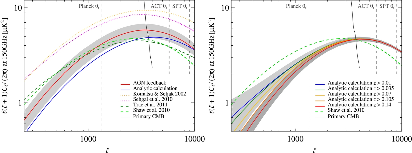
In the left panel of Figure 5, we plot the tSZ power from our analytical halo calculation and that from the AGN simulations. For reference, we include other tSZ power spectrum templates (Komatsu & Seljak 2002; Sehgal et al. 2010; Shaw et al. 2010; Trac et al. 2011). We choose the cosmological parameters for the halo calculation to match the simulations and integrate from z = 0.07 to z = 5, so that the only possible sources of differences are the mass function and the pressure profiles. There are clear differences between the analytical halo calculation and the complete simulation maps. The main difference at low ℓs results from shot noise within the sample of simulated boxes, where we had more (though consistent within the expected error) high-mass clusters than expected, but this is only a 6% effect in the total power spectrum (see Appendix). The differences at higher ℓs arise from deviations about the average pressure profile, including effects of cluster substructure and asphericity. We see these variations in the residual maps of individual simulated cluster projections and pasted-profile projections (see Figure 3). We further explore these differences in the power spectrum between the analytic calculation and the simulations in the following Sections 5.1 and 5.2. It is challenging to determine the causes for all the differences between our calculations and other calculations for the tSZ power spectrum (Komatsu & Seljak 2002; Sehgal et al. 2010; Shaw et al. 2010; Trac et al. 2011), since the thermal pressure profile we use is different from the ones used by the other calculations. However, the reasons for the differences we find between our three methods will be generally applicable to the other methods of calculating the tSZ power spectra.

Figure 5. In the left panel, we show a comparison of the current predictions for the tSZ power spectra at 150 GHz from our simulations with AGN feedback (red line) and the analytical calculations using the constrained pressure profiles in this work (blue line). The standard deviation among our 10 simulations is shown with a light gray band. We also include the semianalytical simulations by Sehgal et al. (2010, pink dotted line) and Trac et al. (2011) which includes enhanced non-thermal pressure support (dark green dashed line) and the fully analytical calculations by Komatsu & Seljak (2002, orange dotted line) and Shaw et al. (2010, light green dashed line). The full width at half-maximum values appropriate for the Planck, ACT, and SPT beams are also plotted. At low-ℓ, our two methods of calculating the tSZ diverge because our simulations happen to contain a large number of high-mass objects driving the power up, though the excess is consistent with expected Poisson fluctuations. At high-ℓ, the discrepancy is the result of substructure and asphericity, as demonstrated in Sections 5.1 and 5.2. The right panel shows a comparison between the current analytic calculations for the tSZ power spectra and how the power spectrum changes with the variation of the lower redshift limit of integration. The variance of 1% of the full-sky power spectrum (see Equation (7)) is illustrated by the gray bands for the highest and the lowest redshift limits of integration.
Download figure:
Standard image High-resolution imageThe right panel of Figure 5 shows a direct comparison between our analytical model and the Shaw et al. (2010) model. In both calculations, the same cluster mass function was used and the power spectra are scaled to the same cosmological parameters, so the differences are related to the model for the thermal pressure profile. We investigate the redshift integration limits,11 but find they do not significantly affect the differences at ℓ ≳ 1000. We present the expected mean and standard deviation of 1% of a full-sky tSZ measurement as a function of lower redshift cutoff, and find that the low-ℓ variance is substantially suppressed by raising the low-z cutoff. On the scales where the tSZ peaks, we find both the mean spectrum and the variance are only weakly affected by varying the redshift limit from z = 0.01 to z = 0.14. Similar results have been found when making intensity cuts on sky maps (Shaw et al. 2009).
We now present power spectra calculated directly from the simulations. In addition to projecting the full electron pressure from all particles, we also take advantage of the information from the simulation cluster catalogs. By doing this, we can employ mass, redshift, and radius cuts to explore the dependence of the full tSZ power spectrum. By pasting our global pressure profile to locations and redshifts of simulated clusters, we can also explore, without having to worry about sample variance, the effects of using our profile instead of the full simulation results.
We use the cluster catalogs described in Section 4.1, and remind the reader that MFOF is roughly equal to M200, though with large scatter.12 Our cluster mass function becomes incomplete below M200 ∼ 4 × 10¹³ M☉ (see Appendix) primarily due to our MFOF cutoff in the original cluster finding of 1.4 × 10¹³ M☉, but partially due to the linking length merging some clusters/groups into nearby larger clusters at the 10%–15% level (e.g., Davis et al. 1985; Bertschinger & Gelb 1991; Cole & Lacey 1996; Cohn & White 2008). For these reasons, we examine only cluster with M500 > 4.2 × 10¹³ M☉ when we bin clusters in mass.
In the left panel of Figure 6 we show the cumulative distribution function (CDF) for the tSZ power for a CDF(M >, z < ) at ℓ = 3000. The CDF illustrates where the relative amount of power originates at the 25%, 50%, and 75% percentile levels. Half the power at ℓ = 3000 comes from clusters with z > 0.6 and half originates from clusters with mass M500 < 2 × 10¹⁴M☉. This result is in general agreement with other work (Komatsu & Seljak 2002; Trac et al. 2011). We note that the particulars of these mass and redshift ranges are sensitive to the input modeling of the ICM. In the right panel of Figure 6, we show the fractional contribution to the power spectrum at ℓ = 3000 per unit redshift per decade in mass for the analytic power spectra. The comparatively low mass and high redshift of the clusters and groups that make up the bulk of the tSZ signal mean that they have not been as well studied as more massive and nearby objects. Thus, the tSZ angular power spectrum can provide a statistical constraint on the astrophysical processes of importance at high-redshift and in low-mass clusters.

Figure 6. Left: shown is the cumulative distribution function for the thermal SZ power spectrum of our AGN simulations as a function of mass and redshift at ℓ = 3000. The curves show the lower mass and upper redshift cutoffs that contribute [25, 50, 75]% to the tSZ power spectrum. At ℓ = 3000, half the power of tSZ power spectrum comes from clusters with z > 0.6, and half comes from clusters with M500 < 2 × 10¹⁴ M☉. For comparison, the dashed green lines show the semianalytical results of Trac et al. (2011), which include enhanced non-thermal pressure support. Right: the fractional contribution to the analytic SZ power spectrum at ℓ = 3000 as function of redshift and log10 M500. The black contours in the right panel contain 25%, 50%, and 75% of the SZ power at ℓ = 3000. The color scale is the fractional contribution to the total spectrum per unit redshift and per decade in mass.
Download figure:
Standard image High-resolution image5.1. Contribution to the tSZ Power Spectrum in Cluster Mass Bins
In this subsection, we calculate the power spectrum in mass bins. This allows us to isolate the differences between the simulations, the pasted-profile maps, and the analytic calculation, as functions of cluster mass, integrating in redshift between z = 0.07 and z = 5. We explore both, cumulative and differential mass bins. We consider all gas particles (or radii) within 6R500 when projecting the thermal pressure of the simulations. Our method takes care of not double counting the cluster mass in overlapping volumes of close-by clusters. In Figure 7, we show the power spectrum broken down into cumulative (left panel) and differential (right panel) mass bins. The bottom panels show the relative differences, where  , with Cℓ, sim denoting the power spectra from the simulations and the Cℓ, i are the power spectra from either the projected pasted-profile maps or the analytic calculation.

Figure 7. tSZ power spectrum sorted into bins of cluster mass. Left: we show the cumulative tSZ power spectrum in mass bins (Cℓ, tSZ (M500 > Mcut) from the AGN feedback simulations, the pasted-profile maps, and the analytical calculation. Right: we show the differential tSZ power spectrum Cℓ, tSZ (Mcut, low < M500 < Mcut, high) for the same power spectrum calculations. In the bottom of both panels we show the relative difference,  , where Cℓ, sim is the power spectrum of the simulated maps and Cℓ, i is that from the pasted-profile maps and the analytical calculation. The differences between the simulations and the pasted-profile maps result from the absence of substructure and asphericity in the pasted-profile maps, which is larger for more massive clusters. The larger differences found between the analytical calculation and the simulations are the result of the mass catalog of the simulations having an excess of high-mass clusters and deficit of lower mass cluster compared to the analytic mass function (see Figure 11).
Download figure:
Standard image High-resolution imageThe largest deviations between our analytic/pasted-profile spectra and the full simulations are for the highest mass (M500 ≳ 4.2 × 10¹⁴M☉) clusters, particularly on small angular scales. The deviations between the pasted profiles and the simulations in this mass range arise from the increased level of substructure and asphericity in massive clusters in comparison to smaller objects due to the more recent formation epoch of large systems in a hierarchical structure formation (Wechsler et al. 2002; Zhao et al. 2009; Pfrommer et al. 2011; BBPS1). The high-mass difference between the fully analytic tSZ spectrum and the simulation results reflects our overabundance of high-mass clusters due to shot noise relative to the mass function used in the analytic calculation. The agreement between all three methods is excellent for masses below 4.2 × 10¹⁴ M☉ until our cluster catalog becomes incomplete at low masses. In the most massive cluster bin, the relative differences between the power spectra are ∼40%–60% for ℓ ∼ 2000–9000 (see Figure 7). For the lower mass bins the differences fluctuate between ±30%, with the pasted profiles generally agreeing better with the full simulation results.
5.2. Contribution to the tSZ Power Spectrum in Redshift Bins
In this subsection, we calculate the power spectrum in redshift bins and compare the results from the simulation, the pasted-profile maps, and the analytical calculation to aid in understanding the differences between these approaches. In Figure 8, we show the power spectrum broken down into cumulative (left panel) and differential (right panel) redshift bins. Here we fix the mass range to M500 > 4.2 × 10¹³ M☉ and set the lower redshift integration bound for the cumulative spectra to z = 0.07. We use the same definition for ΔCℓ to show the differences between power spectrum calculations. In contrast to the mass cuts, the differences between the projected simulated maps and the pasted-profile maps are similar across all the redshift slices (see Figure 8). For ℓ < 5000, there is a ∼5%–10% difference between the pasted profiles and the simulations, rising to ∼20% at ℓ = 10, 000. These results suggest that the contributions from substructure and asphericity to the power spectrum are similar across the redshift range explored, with the exception of one redshift bin z ∼ 0.4 which contains a rare merger event. The large deviations between the analytic and simulation/profile-paste spectra in the highest redshift bin are likely due to the incompleteness of the cluster catalogs at the lowest masses, which are preferentially more important at high redshift. At low redshift, we attribute the difference between the analytic and the profile-paste power spectra to the shot noise in the most massive clusters.

Figure 8. Same as Figure 7, however for redshift slices. Left: we show the cumulative tSZ power spectrum in redshift bins Cℓ, tSZ (z < zcut) from the AGN feedback simulations, the pasted-profile maps, and the analytical calculation. Right: we show the differential tSZ power spectrum Cℓ, tSZ (zcut, low < z < zcut, high) for the same power spectrum calculations. In the bottom of both panels we show the relative difference,  , where Cℓ, sim is the power spectrum of the simulated maps and Cℓ, i is that from the pasted-profile maps and the analytical calculation. The agreement between the pasted-profile and simulation spectra is excellent below ℓ ∼ 5000 for all redshifts. On smaller scales, cluster substructure contributes similarly across all redshift bins examined.
Download figure:
Standard image High-resolution image5.3. Contribution to the tSZ Power Spectrum within Given Cluster Radii
In this subsection we apply radial truncations to the full simulated pressure maps, using clusters with M500 > 4.2 × 10¹³ M☉ at 0.07 < z < 5. The procedures for making real-space radius cuts in maps or analytical calculations are not trivial, since any sharp cut in real space produces ringing in Fourier space, potentially transferring power from large to small angular scales. To reduce ringing and the potential to artificially increase the high-ℓ power spectrum, we use a Gaussian taper when truncating the pressure profile. We place radial tapers at r = R500, 2R500, 3R500, and 6R500 in the maps, adopting 6R500 as the reference radial taper.13 The form of the taper is

for r greater than the taper radius rt, and unity otherwise. In the bottom panel of Figure 9 we show the relative difference,  , where
  is the power spectrum from the 6R500 radial cut and Cℓ, i are power spectra from the other radial cuts. The trend we find is that the large radii of clusters are only important for the low ℓs, for example, the contributions to the tSZ power spectrum when only integrating out to R500 yields ∼30%–65% of the total power from ℓ = 100 to 1000, respectively. At ℓ = 3000 only about 10% of the total tSZ power comes from beyond R500. This number is consistent with previously quoted values (Sun et al. 2011). We note that there is some small residual Fourier ringing, as the tapered spectra rise above the fiducial at ℓs of many thousand. Nevertheless, at higher ℓ, the cluster centers begin to be resolved and become the dominant contributors to the tSZ spectrum since their surface brightnesses are so much larger than any emission in the cluster outskirts.

Figure 9. Cℓ, tSZ (r < Rcut) for the AGN feedback simulations. The thermal pressure distribution has been tapered as in Equation (13) at varying cluster-centric radii before projection. On small scales, virtually all of the power at ℓ > 2000 comes from r < 2R500. About 80% of the tSZ power is recovered at ℓ = 3000 when tapering at R500, though the deviations become substantially larger at smaller ℓ. These results emphasize the importance of understanding cluster pressure profiles well past R500 in order to do high-precision work with the tSZ power spectrum.
Download figure:
Standard image High-resolution image6. CONSTRAINTS OF σ8 FROM CURRENT ACT AND SPT DATA
Using the tSZ power spectrum and ignoring any template uncertainty, the constraints on σ8 are competitive with other cosmological measurements. After accounting for template uncertainty, there is no statistically significant discrepancy between σ8 determined from the tSZ power and that derived from primary CMB anisotropies, or the other measurements (Dunkley et al. 2010; Shirokoff et al. 2010). Here we use our Cℓ, tSZ templates at the fiducial parameters σ8 = 0.8 (and Ωbh = 0.03096) to define the shape of the tSZ power spectrum, and content ourselves with determining only the template amplitude, AtSZ, relative to that expected from the background cosmology (e.g., Battaglia et al. 2010; Dunkley et al. 2010). The amplitude of AtSZ is proportional to a large power of σ8 (AtSZ∝σ7...98; Bond et al. 2002, 2005; Komatsu & Seljak 2002; Trac et al. 2011). It follows that values of AtSZ below unity imply that theoretical templates overestimate the SZ signal, or else points to a smaller value of σ8 than the value derived from primary CMB anisotropies.
The probability distributions of the amplitude, AtSZ, and other cosmological parameters are determined from current CMB data using a modified version of CosmoMC (Lewis & Bridle 2002), which uses Markov Chain Monte Carlo techniques. We include data from WMAP7 (Larson et al. 2010) and, separately, ACT (Das et al. 2011) and the dusty star-forming galaxy-subtracted data from SPT (Shirokoff et al. 2010). We fit for six basic cosmological parameters (Ωbh2, ΩDMh2, ns, the primordial scalar power spectrum amplitude As, the Compton depth to re-ionization τ, and the angular parameter characterizing the sound crossing distance at recombination θ) with the assumption of spatial flatness. Following Dunkley et al. (2010), we include a white noise template for point sources Cℓ, src with amplitude Asrc. The primary difference between our analysis and the analysis by SPT (Shirokoff et al. 2010) is that we marginalize over Asrc, allowing for arbitrary (positive) values, and ignore the spatial clustering component of point sources. We assume a perfect degeneracy Cℓ, kSZ∝Cℓ, tSZ for the kSZ component, so we only need the relative amplitude of AkSZ/AtSZ at a given frequency and use the kSZ amplitudes from Battaglia et al. (2010), where the ratio of kSZ to tSZ at ℓ = 3000 and 150 GHz is 0.44. As mentioned in Battaglia et al. (2010), these simulations do not fully sample the long-wavelength tail of the velocity power spectrum and do not include any contributions from patchy re-ionization (Iliev et al. 2007, 2008). Hence this kSZ power spectrum template is a lower limit to the total power.
In Figure 10, we illustrate the 68% allowed confidence intervals for the tSZ power spectrum, given the shape of our AGN feedback template, our predicted tSZ-to-kSZ power spectrum ratio, and the current data from ACT and SPT. We scale our template using the best-fit σ8 value from Keisler et al. (2011) of 0.814 and scale our template (which was calculated at σ8 = 0.8) by (0.814/0.8)8, about 15%. We find that our template is within about the 68% confidence interval region for both ACT and SPT (see Table 2), after correcting for our predicted kSZ-to-tSZ power spectrum ratio of 0.44. Note that the semianalytic and analytic models without substructure have lower tSZ amplitudes, which would result in higher values of AtSZ and higher σ8.

Figure 10. Our 150 GHz tSZ power spectrum of our AGN feedback model, rescaled to the Keisler et al. (2011) best-fit σ8 value of 0.814 (red line) is contrasted with the bands indicating the 68% range in tSZ amplitude from ACT (Das et al. 2011, dark gray) and SPT (Shirokoff et al. 2010, light gray). For comparison, we plot several other models for the tSZ power spectrum, also shifted to the fiducial σ8 = 0.814. These are Sehgal et al. (2010, pink dotted line), Trac et al. (2011, dark green dashed line), Komatsu & Seljak (2002, orange dotted line), and Shaw et al. (2010, light green dashed line). We include the estimated beam FWHM for ACT, SPT, and Planck.
Download figure:
Standard image High-resolution imageTable 2. Cosmological Constraints on AtSZ and σ8 from ACT and SPT Using the AGN Feedback tSZ Power Spectrum Template
| Data | AtSZ | σ8 |
|---|---|---|
| ACT (Das et al. 2011) | 0.85 ± 0.36 | 0.784+0.036−0.053 |
| SPT (Shirokoff et al. 2010) | 0.69 ± 0.29 | 0.764+0.035−0.051 |
Download table as: ASCIITypeset image
7. DISCUSSION AND CONCLUSION
In this work, we found a global fitting function for cluster thermal pressure profiles using the simulations presented in Battaglia et al. (2010). We find that this global fit matches the mean pressure profiles across mass and redshift generally to an accuracy of better than 10%. We have used the profile fit to reconstruct the tSZ power spectrum using both fully analytic and semianalytic pasted profiles onto cluster position in the simulations, and find we recover the tSZ power spectrum to ∼15% at ℓ = 3000 (see Figure 5). Other analytic and semianalytic models for the tSZ effect commonly assume a constant logarithmic slope of the P–ρ relation, Γ, when solving the equation of HSE. The assumption is not borne out in our simulations, where both the thermal Γ (which account only for the thermal pressure) and the effective pressure Γ (which includes non-thermal support from bulk flows in clusters to the pressure) considerably increase in cluster outskirts (see Figure 6). Using both the simulations and the global pressure profile, we examined the contributions to the tSZ spectrum as functions of cluster mass, redshift, and truncation radius. We found that the contributions from substructure and asphericity are most important for the highest mass clusters (M500 ≳ 4.2 × 10¹⁴ M☉), but remain significant at the 10%–15% level across all mass bins. We find that half the power of the tSZ power spectrum at ℓ = 3000 is contributed by clusters with z > 0.6 and half the power originates from clusters with M500 < 2 × 10¹⁴ M☉.
We have compared our tSZ prediction to results from the ACT and the SPT. We found that there is no statistically significant difference between our model and the data, after accounting for a simplistic correction from the kSZ effect. More complete component separation should be possible with better frequency coverage (Millea et al. 2011). We note that our analysis differs from that in Shirokoff et al. (2010) in that we make no prior assumption about the amplitude of the point-source power spectrum, other than that it is non-negative.
The pressure profile presented in this work is derived from the mean electron pressure in our simulations and, as such, is appropriate for comparison with individual clusters; we defer the derivation of a mean profile designed to include the effects of substructure and asphericity in the power spectrum to future work. This profile will not be expected to match individual cluster observations, but we hope will allow analytic calculations of the tSZ power spectrum to an accuracy of significantly better than 10%. With future data sets, such as those expected from Planck, ACTpol, and SPTpol, it may be possible to constrain not just the amplitude but the shape of the tSZ spectrum. In this case, analytic calculations may be usable to constrain not just cosmology but the important astrophysical processes in clusters with the tSZ effect. Doing so through the power spectrum has the advantage that it is sensitive to lower mass and higher redshift clusters as well as cluster outskirts in ways that are complementary to other data sets.
We thank Norm Murray, Neal Dalal, Mike Nolta, Phil Chang, Hy Trac, Diasuke Nagai, Laurie Shaw, Doug Rudd, Gus Evrard, and Graeme Addison for their useful discussions. Research in Canada is supported by NSERC and CIFAR. Simulations were run on SCINET and CITA's Sunnyvale high-performance computing clusters. SCINET is funded and supported by CFI, NSERC, Ontario, ORF-RE, and UofT deans. C.P. gratefully acknowledges financial support of the Klaus Tschira Foundation. We also thank KITP for their hospitality during the galaxy cluster workshop. KITP is supported by National Science Foundation under Grant No. NSF PHY05-51164.
APPENDIX: COMPARING THE CLUSTER MASS CATALOG TO THE MASS FUNCTION
In this Appendix, we compare the mass function from our simulations with that of Tinker et al. (2008). Our cluster mass catalogs were made with spherical overdensity mass with respect to the critical density and the mass function is with respect to the mean matter density. So, we converted the M200 from the simulations to M200, m assuming the mass profile is dominated by dark matter and use the concentration–mass relations from Duffy et al. (2008). We show in Figure 11 that there is a clear deficit of low-mass clusters due to the chosen linking length of 0.2 in our FOF finder. At this length, it is well known that neighboring clusters are sometimes artificially merged together (e.g., Davis et al. 1985). We also instituted a firm lower limit mass cutoff in the initial FOF catalogs of MFOF > 1.4 × 10¹³M☉, and so our mass function is also expected to be incomplete near that mass.

Figure 11. We compare the mass function, dn/dM, for the cluster catalog from AGN feedback simulations to the mass function from Tinker et al. (2008). The differences at high masses indicates that in the 10 independent simulations we happen to have more high-mass clusters than is expected on average (though with only six with M500 > 7.1 × 10¹⁴ M☉ this is consistent with shot noise). At low masses, our catalog is incomplete due to our FOF halo finding (see the text).
Download figure:
Standard image High-resolution image
There is a clear excess of high-mass clusters in our simulations, but it is consistent with shot noise (we only have six clusters with M500 > 7.1 × 10¹⁴ M☉). We now estimate the excess power in our full simulation power spectrum due to this upward fluctuation in the highest mass bin. Where the cluster catalogs are complete, we expect that over an enormous number of simulations, the paste profile and analytic calculation of the tSZ power spectrum would converge, and indeed see the agreement is excellent between the two in the right panel of Figure 7 for all but the lowest (due to catalog incompleteness) and highest (due to shot noise) mass bins. We therefore adopt the ratio of the pasted-profile spectrum to the analytic spectrum as a quantitative estimate of the over-representation of high-mass clusters in our finite number of realizations. At ℓ = 3000 this ratio is 2.0 for clusters with M500 > 7.1 × 10¹⁴ M☉, though as can be seen in Figure 7 the specific value is insensitive to the reference ℓ. Since the high-mass contribution to the tSZ spectrum from the full simulation projections is 0.67 μK2 at ℓ = 3000, in the limit of an infinite number of simulations, we would expect the average contribution from clusters with M500 > 7.1 × 10¹⁴M☉ to be 0.34 μK2 lower. The total power spectrum at ℓ = 3000 is 5.78 μK2, so this shot noise correction amounts to just less than a 6% shift in the total power spectrum.
Footnotes
- 6
- 7
Note that we are not including the contributions from the clustering of clusters, since this is sub-dominant on scales of ℓ > 300 (Komatsu & Kitayama 1999).
- 8
Here we have ignored the temperature of the CMB, TCMB, since TCMB ≪ Te, hence ne kB(Te − TCMB) ≃ ne kB Te = Pe.
- 9
Some older models have ignored kinetic support entirely, in which case Ptot = Pth.
- 10
We have selected the redshifts at which we write out the simulation snapshots to be the light crossing time of the simulation; hence, the total power spectrum is the sum of the differential power spectra.
- 11
For the remainder of this paper, we use a low-redshift cutoff of z = 0.07, so that we can directly compare our analytic calculation to the simulations.
- 12
For detailed work on comparing the mass definitions of MFOF to MΔ and the resulting halo mass catalogs from these definitions, see More et al. (2011), and the references therein.
- 13
We avoid double counting gas particles when we project them into maps. If a particle lies in the overlap region between two clusters, we taper the particle with the larger of the two possible taper values, i.e., those particles with a smaller radius R/R500, to avoid artificially suppressing power in the overlap region.