


ABSTRACT
This second paper of the series investigates the transverse response of a magnetic field to the independent relaxation of its flux tubes of fluid seeking hydrostatic and energy balance, under the frozen-in condition and suppression of cross-field thermal conduction. The temperature, density, and pressure naturally develop discontinuities across the magnetic flux surfaces separating the tubes, requiring the finite pressure jumps to be compensated by magnetic-pressure jumps in cross-field force balance. The tangentially discontinuous fields are due to discrete currents in these surfaces, δ-function singularities in the current density that are fully admissible under the rigorous frozen-in condition but must dissipate resistively if the electrical conductivity is high but finite. The magnetic field and fluid must thus endlessly evolve by this spontaneous formation and resistive dissipation of discrete currents taking place intermittently in spacetime, even in a low-β environment. This is a multi-dimensional effect in which the field plays a central role suppressed in the one-dimensional (1D) slab model of the first paper. The study begins with an order-of-magnitude demonstration that of the weak resistive and cross-field thermal diffusivities in the corona, the latter is significantly weaker for small β. This case for spontaneous discrete currents, as an important example of the general theory of Parker, is illustrated with an analysis of singularity formation in three families of two-dimensional generalizations of the 1D slab model. The physical picture emerging completes the hypothesis formulated in Paper I that this intermittent process is the origin of the dynamic interiors of a class of quiescent prominences revealed by recent Hinode/SOT and SDO/AIA high-resolution observations.
Export citation and abstract BibTeX RIS
1. INTRODUCTION
This series of papers investigates the unlimited hydromagnetic steepening of magnetic field gradients under the frozen-in condition. An infinite field gradient as a mathematical singularity is physically admissible under a rigorous imposition of that condition. In the solar corona, with its extremely high but finite electrical conductivity, this steepening would proceed only to such extreme but finite gradients at which the frozen-in condition ceases to be a valid approximation. In this manner a coronal field may be in a stable equilibrium globally while it undergoes this breakdown of the frozen-in condition in many localities (Parker 1994; Low 2007; Low & Janse 2009; Janse & Low 2009). At each breakdown, the intense electric current density dissipates resistively and the magnetic field reconnects. Once the extreme field gradients are thus removed, a high degree of frozen-in condition is restored, only to bring about further field steepening (Janse & Low 2010). We hypothesize that this process, intermittent in spacetime, is the origin of the restless dynamical interiors of quiescent prominences, of the polar-crown type, revealed by high-resolution Hinode/SOT and SDO/AIA observations (Martin et al. 1994; Tandberg-Hanssen 1995; Gaizauskas 1998; Labrosse et al. 2010; Mackay et al. 2010; Berger et al. 2008, 2010, 2011; Okamoto et al. 2007, 2010; Liu et al. 2012).
In the first paper (Low et al. 2012, hereafter Paper I), we treat the thermally balanced one-dimensional (1D) Kippenhahn–Schlüter (KS) slab (Kippenhahn & Schlüter 1957; Low 1975; Low & Wu 1981; Zweibel 1982; Low & Zhang 2004; Hillier et al. 2011). This is an infinite vertical slab of plasma supported against gravity in a bowed magnetic field under the frozen-in condition and subject to a steady transport-equation balancing theoretically defined optically thin radiative loss, volumetric heating, and heat conducted along the field. For a sufficiently large total mass per unit magnetic flux, force and energy balance requires a fraction of that mass in a magnetic flux tube to have collapsed into a cold dense core at the tube's lowest point. This core is a δ-function singularity in fluid density. The δ-function cores on adjacent thin flux tubes form a discrete surface, a zero-thickness sheet with a finite mass per unit area threaded across by the bowed field. A corresponding δ-function in electric current density, a discrete current, flows in this mass sheet such that its Lorentz force balances the weight of the mass sheet. This discrete current can persist only if the electrical conductivity is infinite. In the presence of an extremely large but finite conductivity, this current dissipates resistively upon formation, producing heating and resistive cross-field flows as we have also modeled in Paper I.
In this second paper, we show that the intermittent frozen-in breakdown is greatly enhanced and spatially pervasive when the magnetic field plays an active dynamical role possible only in multi-dimensional systems. This is a formidable time-dependent problem not well understood. Therefore, we continue with the methodology used in Paper I of demonstrating a general inevitability of discrete currents in equilibrium states when the frozen-in condition is rigorously imposed. These discrete currents indicate where the frozen-in breakdown would occur if the fluid of a large but finite electrical conductivity evolves in search of equilibrium. The cross-field balance of forces and energy in the 1D KS slab is simple, with the physical problem reduced to just the balance along the field. Its flux tubes of equal magnetic flux are all identical. Temperature is automatically continuous across the field, and the magnetic suppression of thermal conduction across the field has no cross-field consequences. In sharp contrast, the consequences arising from zero cross-field thermal conduction are far reaching in multi-dimensional fields.
In two-dimensional (2D) and three-dimensional (3D) fields, flux tubes of the same unit axial flux generally are topologically and geometrically different and loaded with different masses. Without thermal conduction across the field, each flux tube determines its tube-aligned temperature distribution according to its field-aligned energy transport, independent of the tubes contiguous to it. In the relaxation of such a hydromagnetic system to static equilibrium under the frozen-in condition, the temperature naturally becomes discontinuous across very many magnetic flux surfaces. Consequently, the pressure is generally also discontinuous across these surfaces in the equilibrium available. For 2D and 3D equilibrium fields, that fluid-pressure jump is balanced by an equal and opposite jump in magnetic pressure, readily accommodated in the magnetically dominated corona. The latter jump implies discrete currents flowing in entire flux surfaces. A complexity of discrete currents extending pervasively in the fluid thus develops during evolution, quite separate from the other kind of discrete currents at collapsed mass sheets found in Paper I. All discrete currents dissipate in a real fluid by its small, nonzero resistivity when field gradients have steepened sufficiently. The field reconnects and diffuses across fluid surfaces, with the overloaded, reconfigured flux tubes falling by gravity and the underloaded ones rising by magnetic buoyancy. This implied scenario is suggestive of the Hinode/SOT and SDO/AIA movies of the interiors of quiescent prominences (Berger et al. 2008, 2010; Liu et al. 2012).
The hydromagnetic property we investigate is a novel application of the Parker theory of spontaneous current sheets (Parker 1972, 1990, 1991, 1994; Petrie & Low 2005; Janse & Low 2010; Janse et al. 2010). The Parker theory concentrates on explaining the quiescent heating of the corona by investigating the force-free magnetic field, a field with zero Lorentz force in a fluid of negligible inertia. The preservation of the field topology under the frozen-in condition can force the embedding fluid to be torn tangentially on flux surfaces, producing discrete currents, in order to render the field force-free. Since fluid pressure is neglected, force balance requires the continuity of the magnetic pressure everywhere. This leaves the field direction to be discontinuous as a degree of freedom to admit discrete currents. The essence of the Parker theory is that in most 3D situations, discrete currents are generally inevitable because in their absence no continuous current density on its own can ensure that the field in equilibrium has exactly the topology it possesses for all time. The prominence field presents the same basic inevitability for discrete-current formation, to ensure field-topology invariance under the frozen-in condition in a more complicated situation, that of balancing the Lorentz force with the pressure and gravitational forces.
We organize our paper to first concentrate on the basic hydromagnetic effects. Section 2 formulates an elementary theory based on a set of 2D magnetostatic equations for a thermally balanced fluid assuming zero cross-field thermal conduction. Section 3 presents a justification of that assumption in terms of the Spitzer (1962) thermal-conduction and electrical diffusivities in a fully ionized gas. Section 4 presents three families of idealized magnetostatic solutions that together illustrate different aspects of inevitable discrete currents in equilibrium states. Section 5 relates this study to the observed quiescent prominences. We use cgs units in this paper.
2. MAGNETOSTATIC EQUILIBRIUM
We derive the 2D magnetostatic equations describing a fluid of perfect electrical conductivity that thermally conducts heat along but not across the magnetic field. The field-aligned thermal conduction steadily balances a heat source and a radiative sink distributed in the fluid. In Section 3, we analyze the physical values of thermal and electrical conductivities expected in the corona to examine when the separate assumptions of the frozen-in condition and the zero cross-field thermal conduction may break down.
2.1. The Magnetostatic Equations in 2D
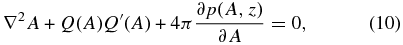
We adopt the following one-fluid hydromagnetic description of the corona and prominence:
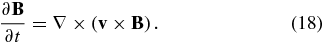
where v, B, ρ, p, and g denote, respectively, the velocity, magnetic field, density, pressure, and uniform gravitational acceleration in the negative Cartesian z-direction. We also need an equation of state and another for energy transport, the latter involving anisotropic thermal conduction, radiative processes, and volumetric heating operating in the corona. If these energy processes are specified explicitly in terms of the fluid and field variables, Equations (1)–(3) together with the scalar equations of state and energy transport are a complete set to determine these variables, including the temperature T.
For simplicity in our analysis of basic effects, we neglect viscosity in momentum equation (1) and take electrical conductivity to be isotropic, characterized by a constant σ related to the resistivity η = c2/4πσ, where c is the speed of light. The length scale l0 ≈ 7 × 107 cm is of the order of spatial resolutions achievable in solar observations from the ground. In the corona and prominence interior, the resistive diffusion of a magnetic field of that length scale has a timescale τD = l20/η of tens of years and longer if σ is estimated with the formula of Spitzer (1962) in the temperature range of 104–106 K for a fully ionized gas. Therefore, for dynamical events in the corona and prominences observed over timescales of hours at spatial resolutions not drastically smaller than l0, the frozen-in condition is an excellent approximation with an important qualification. There can be processes, unresolved in such observations, creating field structures of sufficiently small scales over which resistive dissipation is significant. The observable large-scale consequences of this dissipation are not possible to be described under the frozen-in condition. For example, at the large scales of resolution-limited observations, a significant larger "effective" resistivity may appear to be operating. This general physical point important for understanding quiescent-prominence observations is a central motivation of this series of papers.
2.2. Thermally Balanced Equilibrium States
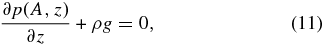
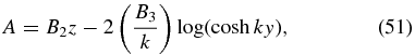
Consider the relaxation of a fluid to static equilibrium under the frozen-in condition, setting η = 0. This equilibrium is described by

In addition to force balance, we have thermal balance among a radiative-loss sink  , a heating source
  , and a field-aligned thermal flux with conductivity κ, all these quantities assumed to be expressible as known functions of the fluid and field. We assume the ideal gas law, kB and m0 being the Boltzmann constant and the mean molecular mass, respectively.
Consider a 2D Cartesian system with the solenoidal field
in terms of the flux function A constant along each field line and an x-component Q, x being an ignorable coordinate. The electric current density J = (c/4π)∇ × B is given by
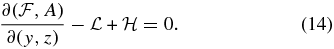
The equilibrium Lorentz force cannot have an x-component, requiring Q(y, z) = Q[A(y, z)] so that Equation (4) reduces to the two components in the y − z plane,
for force balance across and along the field, respectively (Low 1975).
The condition Q = Q(A), together with Equation (10), implies that in equilibrium the current density takes the form
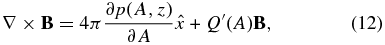
a field-aligned component with a proportionality Q'(A) constant on constant-A field lines and a cross-field component in the x-direction that generates the Lorentz force to balance the forces of pressure and weight. If the latter forces are absent, setting p ≡ 0, we have a force-free field.
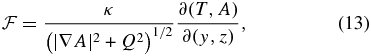
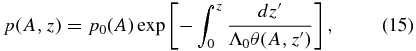
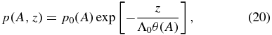
In a stratified atmosphere, we express p(y, z) = p[A(y, z), z], to describe its hydrostatic variation with height z along a constant-A field line. Each point (y, z) on the y − z plane is identified by the value A = A0, a constant, at that point and a height z-varying along the curve A = A0, the way to visualize the partial derivatives of p with respect to (A, z) as independent variables. Henceforth, the dependence of a scalar function on (A, z) shall be indicated when we mean partial derivatives with respect to these variables. The hydrostatic profile of p is subject to the balance of forces across the field lines, the Grad–Shrafanov equation (10).
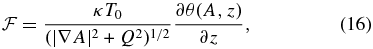
Denote the field-aligned thermal flux in Equation (6) by  , where
introducing the Jacobian operator. Then energy-balance equation (6) takes the form
Equations (7), (10), (11), and (14) constitute a complete system of one algebraic and three partial differential equations (PDEs) determining the four scalar unknowns A, p, ρ, T.
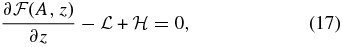
2.3. The Frozen-in Condition
To see the structure of this system of equations, introduce a constant normalization T0, setting T = T0θ and defining the constant hydrostatic scale height Λ0 = kBT0/m0g, using the notations in Paper I. First eliminate ρ between Equations (7) and (11) and then integrate with respect to z, treating (A, z) as the independent variables, to obtain
where p0(A) arises as an arbitrary "constant" in that integration with respect to z. In the representation θ(y, z) = θ(A, z), Equations (13) and (14) take the forms
the latter effectively being an ordinary differential equation balancing a field-aligned thermal conduction against energy loss and gain along each constant-A field line. By using Equations (7) and (15) to express p and ρ in terms of θ, the problem is then reduced to solving Equations (10) and (17) for A and θ as the two coupled unknowns subject to suitable boundary conditions. This is a 2D extension of the 1D KS slab in Paper I.
Taken as a boundary-value problem in PDEs, there are two types of free functions to prescribe in order to render Equations (10) and (17) specific. We must prescribe the thermal conductivity κ, energy sink  , and heat source
  as explicit functions of the fluid and field variables, to identify a specific fluid by its properties. The thermally balanced equilibrium states of this fluid are then generated by all the admissible forms of Q(A) and p0(A), usually called the generating functions. For each pair of analytic [Q(A), p0(A)], the boundary-value problem in the tradition of classical analysis gives either no solution, because the governing PDEs are nonlinear, or an everywhere-analytic solution (Courant & Hilbert 1962). The principal result of Paper I is that the set of all everywhere-analytic solutions is a subset of measure zero of the physically admissible thermally balanced equilibrium states. So the same result may be expected in the 2D extension of the model.
If the electrical resistivity η ≠ 0, there is no steady state because the current density would then decay in time. If η = 0, the fluid surface identified as a flux surface of B at any one time remains a flux surface for all time under continuous displacement, the frozen-in condition expressed by the induction equation
This equation implies, in particular,
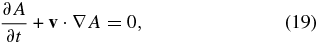
for our 2D system. It is easy to show that as long as v is continuous, setting A(y, z, t) = A0, a fixed constant, describes an evolving fluid surface. Therefore, the total mass M(A1, A2) distributed with x as an ignorable coordinate between any two flux surfaces A = A1 and A = A2, A1 and A2 being constants, is a constant in time. More generally, induction equation (18) states that the net magnetic flux across any fluid surface area is conserved as it deforms continuously. Therefore, the total magnetic flux Φ(A1, A2) contributed by Bx = Q across the area in the y − z plane between two field lines, A = A1 and A = A2, is also a constant in time. When given one of the above 2D thermally balanced equilibrium states, the system must be thought of physically as having arrived at this state with a specific M(A1, A2) and Φ(A1, A2) fixed for the system for all time. If we specify M(A1, A2) and Φ(A1, A2), we are asking for the equilibrium state for a completely identified fluid in terms of its mass and x-directed flux distributed over the constant-A fluid surfaces in some specific manner. For that equilibrium, the functions p0(A) and Q(A) must be given forms that recover M(A1, A2) and Φ(A1, A2), respectively, in the solution. That is, p0(A) and Q(A) are unknowns in this physical formulation of the equilibrium expressed by integral equations that relate them to M(A1, A2) and Φ(A1, A2), respectively; see the discussion of this integro-PDE system by Wu & Low (1987).
Conceptually, M(A1, A2) and Φ(A1, A2) are physical properties that can be freely prescribed. It is thus interesting that, in general, not all prescribed pairs yield an everywhere-analytic solution to their integro-PDE system. The unavoidable singularities in the non-analytic solutions are the weak solutions of the boundary-value problem, meaning that these singularities are not arbitrary but subject to the same physical laws as the integral equivalence to the PDEs governing the continuous part of the global solutions (Courant & Hilbert 1962). From this analysis, an exhaustive search of everywhere-analytic solutions to the boundary-value problems posed by PDEs (7), (10), (11), and (14) with an a priori prescription of continuous p0(A) and Q(A) would miss out on the singular solutions that populate the total set of physically admissible equilibrium states.
Coupling the Grad–Shrafanov equation (10) to the energy-transport equation (17) is an analytically intractable problem. The basic property of interest here is in equilibrium states with a temperature T that is discontinuous across a magnetic flux surface. This effect can be investigated with the simpler equilibrium states in which θ(y, z) = θ(A) with  . Then
  by Equation (16), and energy equation (17) is trivially satisfied. Equation (15) gives
reducing the problem to one of solving the Grad–Shrafanov PDE
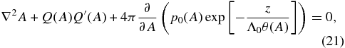
for A with prescribed functions p0(A), Q(A), and θ(A), subject to boundary conditions on A. Since thermal conduction is absent across the field lines, θ(A) is not required to be a continuous function of A. Moreover, the pressure is generally not continuous when the temperature is discontinuous, that is, the function p0(A) may also be discontinuous. The derivatives of p0(A) and θ(A) on the right-hand side of Equation (21) contribute δ-functions to ∇2A and, hence, to the current density given by Equation (9).
All the above magnetostatic problems, as either a purely PDE system or an integro-PDE system, are generally intractable. So we shall make our physical points in Section 4 by specialized solutions to give insights into the general solutions. Before proceeding, we need to address in the next section an important assumption in our analysis. In a real plasma, not only is the electrical conductivity not infinite, that is, there is a small but nonzero resistivity, but its cross-field thermal conductivity is also small but nonzero. The non-dimensional ratio of the resistivity to that thermal diffusion of heat determines whether the breakdown of the frozen-in condition as an approximation precedes the breakdown of the assumption of zero cross-field thermal conduction.
3. THE RESISTIVE AND CROSS-FIELD THERMAL DIFFUSIVITIES IN THE CORONA
The degree of ionization in the optically thin parts of prominences has an observed range of 10−3 to 10−1 (Tandberg-Hanssen 1995; Gilbert et al. 2002, 2007; Labrosse et al. 2010; Mackay et al. 2010). The one-fluid description we have adopted is only a step toward a more complete but formidable description that accounts for the interactions among neutrals, ions, and electrons as separate fluids. Here within the one-fluid description of a fully ionized gas, we demonstrate that cross-field thermal conduction is a weaker effect than electrical resistivity in the corona and prominences.
3.1. The Spitzer Resistivity
We adopt the isotropic, temperature-dependent Spitzer (1962) resistivity,

neglecting for simplicity a weak anisotropy owing to the presence of a magnetic field. We also neglect other complications like the thermoelectric effect on the resistivity arising from an extreme thermal gradient across the field.
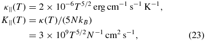
We obtain the values η = 5 × 106 cm2 s−1 at T = 104 K in a prominence and η = 5 × 103 cm2 s−1 at T = 106 K in the corona. The resistive diffusion time τd = L2/η of a magnetic structure of size L = 200 km, representing a lower-limit length scale observable with Hinode/SOT, for example, is of the order of 108 s and 1011 s for the prominence and corona, respectively. These times are too long to be relevant at the timescale of 100 s characteristic of the prominence's vertical threads. Turning the question around, the length scales for which τd ≈ 100 s are LP = 2 × 10⁻¹ km in the prominence and LC = 10−2 km in the corona, both three orders of magnitude, at least, smaller than their respective hydrostatic scale heights of ΛP = 300 km and ΛC = 3 × 10⁴ km.
The mean free paths of the electrons and protons for like-particle collisions have the same dependence on T2/N, where N is the number density of the species. Let us simplify by assuming the same temperature for the two species. Then, this common mean free path is of the order of lP = 5 cm in a prominence plasma of density N ≈ 1011 cm−3 and T = 104 K and lC = 50 km in a coronal plasma of density N ≈ 109 cm−3 and T = 106 K. Therefore, when resistive diffusion in the prominence becomes relevant at a scale of LP = 2 × 10⁻¹ km, this scale is still much larger than the mean free path of lP = 5 cm. On the other hand, because of its high electrical conductivity, resistive diffusion becomes relevant in the corona for scales of LC = 10−2 km or smaller, well below its mean free path of lC = 50 km. In other words, as a field gradient steepens toward a tangential discontinuity under the frozen-in condition, it proceeds until the fluid description breaks down, locally at where the tangential discontinuity is developing without arriving at a resistive fluid regime. The situation is actually more optimistic because in the presence of a 10 G magnetic field, the ions are tied to the field with a cyclotron radius of about 90 cm for protons at T = 106 K, so that the fluid picture may be said to break down only along the field. A proper treatment of this breakdown is outside the scope of the present paper, but it seems reasonable to assume that such a developing tangential discontinuity will excite a host of plasma-kinetic effects to dissipate its growing current density while the fluid description and the frozen-in condition break down. Note that the fluid picture is approximately good along the field to some relatively small scales in the low corona, considering that the mean free path in the corona is of the order of 10−2 of the coronal hydrostatic scale height ΛC.
3.2. The Spitzer Thermal Conductivity
We adopt the Spitzer thermal conductivity and thermometric diffusivity
respectively, taken from Parker (1994), using a subscript to indicate thermal conduction along the magnetic field. The electrons as the carriers of thermally conducted heat are tightly tied to the magnetic field lines. Thermal conduction across the field has the coefficients


greatly reduced from the respective parallel coefficients by a factor of (ωeτe)−2 ≪ 1, where

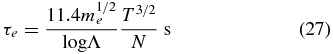
are the electron cyclotron frequency and the time for an electron to be significantly deflected by Coulomb interaction, respectively, in standard notation. For our purpose we set the Coulomb factor log Λ ≈ 10 for application. For example, if the field strength B = 100 G and the electron density is N ≈ 1010 cm−3 at T = 106 K, the cross-field thermal conduction is reduced by a factor of (ωeτ)−2 ≈ 10−10 (Parker 1994). Taking the field to be 10 G, closer to the fields threading quiescent prominences, that reduction factor is still exceedingly small at 10−8.
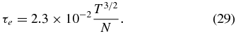
The thermometric diffusivity, K⊥(T), describing the diffusion of temperature, has the same dimension as resistivity η, and we have an interest in their dimensionless ratio. Direct evaluation gives

Then, we have
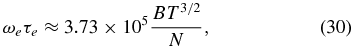
Evaluate the ratio
The quantity p = 2NkBT is just the pressure of the fully ionized gas, which defines the plasma beta
Hence, we have the ratio

The field intensity in a prominence is about 10–60 G, from polarimetric observations (Casini et al. 2003; Lopez Ariste & Casini 2003). If we take N = 1011 cm−3, T = 104 K, and B = 30 G, we get p = 0.28 erg cm−3, β = 7.7 × 10⁻³, and  = 5 × 10⁻³.
With ≪ 1, the thinning of a steep gradient layer to zero will cross the threshold thickness for resistive dissipation of the growing current density in the layer, well before cross-field thermal conduction becomes important. If ≫ 1, the thinning steep gradient will excite cross-field thermal diffusion before resistive diffusion. In this case, the thermal balances in the two adjacent tubes are perturbed and a time-dependent evolution is initiated without breaking the frozen-in condition. It is possible that this evolution on its own develops steep gradient layers even thinner to also excite resistive dissipation. This is just as interesting an outcome, but the case of ≪ 1 is simpler, a clear case of the magnetic thermal insulation directly causing a magnetic tangential discontinuity to form at a flux surface, a novel case of the Parker spontaneous current sheets. Note that β ≪ 1 does not mean that the field is so rigid that it cannot change when the plasma pressure changes. Rather, the field being strong can change by just a small amount to accommodate any plasma-pressure change, including an inevitable jump in the plasma pressure.
4. THREE FAMILIES OF 2D EQUILIBRIUM MAGNETIC FIELDS
Solving equilibrium equations (7), (10), (11), and (14) for A, p, ρ, T in generality requires powerful numerical methods, an undertaking that must be postponed to the future. The 1D KS slab of Paper I is a special case of this system of static equations that is soluble analytically by a reduction of the PDEs to ordinary differential equations. Here we go on to multi-dimensional fields to treat a rich class of inevitable discrete currents distinct from the ones due to the collapsed mass sheets found in the 1D KS slabs. The hydromagnetic effect we aim to understand is, in principle, already identified unambiguously in Section 2. That is, once the temperature is allowed to be discontinuous across a magnetic flux surface under energy equation (14), that surface automatically acquires a discrete current since equilibrium demands for an inevitable tangential field discontinuity across the surface. This consideration shows that the effect in its elementary form is about the cross-field response of a multi-dimensional field to the field-aligned force and energy balance. Only the details of the effect depend on the detailed fluid structures along the flux tubes as demanded by energy equation (14). Here we set out to study how field geometry plays a fundamental role in the multi-dimensional field's response, without having to solve Equation (14) for such details. This is fruitfully done by analyzing the properties of three instructive families of 2D equilibrium states, the solutions in the first family being continuous everywhere and those in the other two families containing inevitable tangential field discontinuities.
4.1. 2D KS Slab with Vertically Periodic Structures
Consider equilibrium in the presence of a spatially uniform temperature. Set θ ≡ 1, that is, T = T0, the uniform temperature, and the Grad–Shafranov equation (21) takes the form

introducing the inverse scale height k0 = 1/Λ0. Let us prescribe


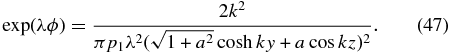
where p1, λ, and B1 are constants. The pressure in Equation (20) takes the form

and the Grad–Shrafanov equation (35) reduces to

The substitution,
transforms the Grad–Shrafanov equation into the Liouville PDE

with the complete integral
introducing u and iv as the real and imaginary parts of an arbitrary analytic complex function F(ω) of the complex variable ω = y + iz, that is,

Each prescription of F(ω) yields a Liouville solution ϕ defining a static equilibrium. The field, with Bx = B1, is given by the flux function (40), frozen into an isothermal density distribution

using the ideal gas law and the pressure (38). The field and density are expressed as functions of space through ϕ(y, z).
For our purpose in this paper, we concentrate on the family of solutions generated by
where k and a are two arbitrary constants. Equation (42) gives the solution
For a given a, define  . Then a transformation y → y + y1 redefines the function ϕ(y, z):
This transformation has moved the origin along the y-axis to a location about which the redefined function ϕ(y, z) is symmetric in y. The free parameter k is the wavenumber of this function's periodicity in z, as well as its exponential decline with y in either direction.
To relate to the physics we are interested in, we prescribe the uniform temperature T0, fixing the inverse scale height k0. Take the free parameter λ to have the dimension of the reciprocal of the field intensity times length. We may then set λ = k0/B2, introducing a constant field intensity B2 to replace λ as a free parameter. We now introduce a third field intensity B3 = (k/k0)B2 to represent the free parameter k as may be convenient to do depending on the physical discussion. Note that λ = k/B3 by definition. Then the magnetic field is given by
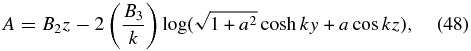
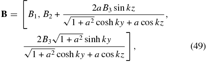
in which (B1, B2, B3) are three field intensities we may arbitrarily prescribe with k = (B3/B2)k0. This is a four-parameter family of everywhere continuous solutions, the fourth being the dimensionless constant a.
Each of these fields is in equilibrium with the isothermal density
which is periodic in z, confined about the central plane y = 0 with an exponential decay over a scale k−1 to zero as y → ±∞. The density is independent of Bx = B1. From force-balance equation (4) with x as an ignorable coordinate, the uniform Bx produces only a uniform magnetic pressure that is immaterial to the force balance. This component plays a more explicit role through the anisotropic influence of the field on thermal conduction in energy equation (6).
4.1.1. The 1D Isothermal KS Slab
Set a = 0 and we have the 1D-slab isothermal solution of Kippenhahn and Schlüter (1957),

Thus, setting a ≠ 0 generalizes this strictly y-dependent solution to vary with both y and z, keeping x as an ignorable coordinate. In Section 4.3 we will be examining a different generalization to 2D, allowing variations in y and x while keeping z as an ignorable coordinate. Therefore, it is useful to see clearly the following specific property of this 1D KS solution as a reference state for these two generalizations.
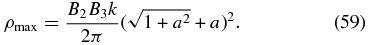
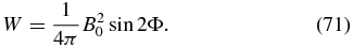
Equation (52) shows that the equilibrium field is the result of weighing down a uniform background field  into a sheared, bowed shape. By the 1D nature of the equilibrium, a measure of the total weight is given by
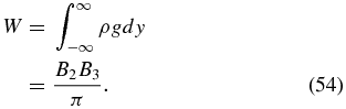
This is the weight in an infinite column of unit cross-sectional area aligned in the y-direction. In the y − z plane, W may be called the integrated weight per unit length in the z-direction, which we henceforth refer to as the weight for brevity. The greater the weight, the greater is the sag defined by Bz = ±2B3 at y → ±∞ for a fixed By = B2. If we hold Bbg fixed, it is useful to replace B3 = πW/B2 with W as a free parameter. Then the wavenumber k = k0B3/B2 can be expressed as k = πk0W/B22, and Equations (51)–(53) read
where we have used k0 = 1/Λ0.
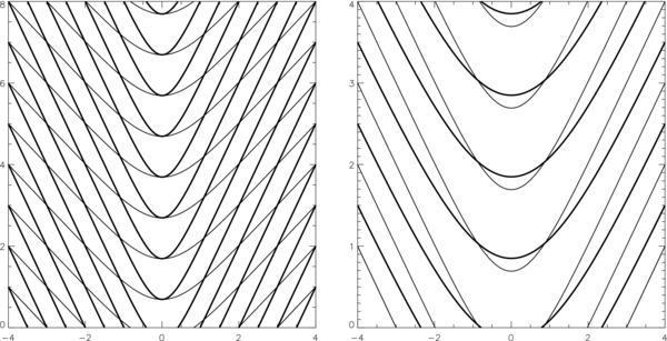
In 3D space, we have an infinite, vertical slab represented by a density ρ(y) symmetrically concentrated about the vertical plane y = 0. The characteristic slab width is B22Λ0/πW. Figures 1 and 2, with a fixed By = B2, suffice for illustrating the parametric dependence of the solution on the isothermal temperature and the total mass W/g in the frozen-in condition.
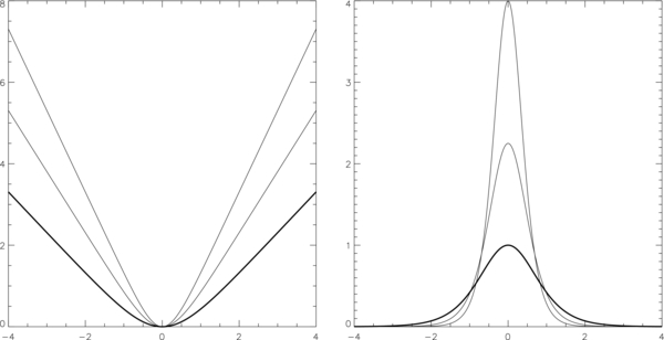
Figure 1. Three solutions for a 1D KS slab with a fixed scale height Λ0 but three increasing values of the total mass W/g defined by Equation (54). With y on the abscissa are the representative field lines each plotted as z(y) (left panel) and their respective density distributions (right panel). The three cases are identified by the properties that the smaller W is, the smaller the maximum density at y = 0 and the flatter the bottom of the bowed field line.
Download figure:
Standard image High-resolution image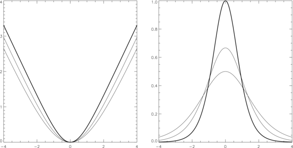
Figure 2. Three solutions for a 1D KS slab with a fixed total mass W/g but three increasing values of the scale height Λ0, in the same format as in Figure 1. The densities in the three cases are identified by the properties that the larger the scale height Λ0 is, the smaller the maximum density at y = 0 with more mass distributed into the wings, and the flatter the bottom of the bowed field line. With the total mass W/g the same for all three solutions, all three field lines at large y tend to the same constant gradient.
Download figure:
Standard image High-resolution imageFigure 1 shows the shapes of the bowed field lines projected on the y − z plane for three slab solutions of increasing values of W, all having the same scale height Λ0. The greater W is, the more inclined the field is below the horizontal indicated by |Bz/By| = B3/B2 = πW/B22 at y → ±∞. The density distributions show the corresponding parametric trend of a narrowing of slab width and an increasing peak value of the density at y = 0. When the total weight W is greater, it weighs more on the background field into a deeper bow such that the slab in equilibrium has a smaller width.
Figure 2 shows the shapes of the bowed field lines projected on the y − z plane for three slab solutions of increasing values of the isothermal temperature T0 and its scale height Λ0, all having the same weight W. Increasing the scale height implies a more gradual spatial decline of stratified density with z along the inclined field. This means that the same total weight W in the three cases is distributed over increasingly thicker slab widths as shown. In all three cases, the field lines tend to the same inclination below the horizontal at y → ±∞ because that inclination is determined by W alone.
4.1.2. The 2D Isothermal KS Slab
If a ≠ 0, we have a 2D KS slab with a slab width k−1 and a periodic vertical structure of wavenumber k. Figures 3 and 4 show four examples with the same values of B2, B3 but with increasing values of a as a measure of departure from one-dimensionality. In each figure, the thin lines are constant-A field lines projected on the y − z plane and the thick lines are contours of constant density. The constant field component Bx = B1 may be taken to be the same for the three examples. This field component does not affect the equilibrium in the y − z plane, but it gives the field, in 3D space, a sheared configuration for the field lines extending to y → ±∞ and a twisted flux-rope configuration for the magnetic islands, or regions of closed field lines, found in Figure 4.
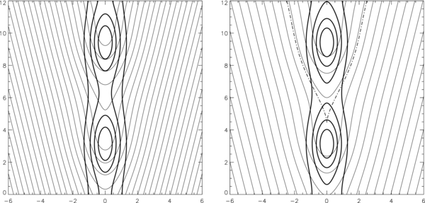
Figure 3. Two solutions of the isothermal 2D KS slab with a = 0.2 (left) and a = 0.25 (right), displayed as vertically periodic thin field lines of constant A and thick contours of constant ρ in the plane with ky on the abscissa and kz on the ordinate. The inverse isothermal density scale height k0 is set to half the wavenumber k of the vertical periodicity, which fixes the critical parameter a0 = 0.25. The equilibrium on the left is an a < a0 state that has only open field lines. The critical a = a0 equilibrium on the right also has only open field lines, but a cusp has appeared on the critical (dashed) field line shown, where O-type and X-type neutral points appear in coincidence.
Download figure:
Standard image High-resolution image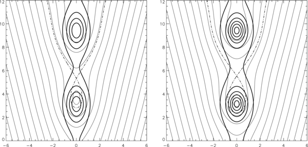
Figure 4. Two solutions of the isothermal 2D KS slab with a = 0.4 (left) and a = 0.6 (right), displayed in the same format as Figure 3, both with k0/k = 0.5 and a0 = 0.25. These a > a0 states have magnetic islands of closed field lines nested around an O-type neutral point and looped around by the infinitely long (dashed) separatrix field line associated with the X-type neutral point shown.
Download figure:
Standard image High-resolution imageFor a < a0 = B2/2B3, all the field lines extend to infinity and are unevenly bowed because the loaded mass per unit magnetic flux varies across the field, the cases in Figure 3. For a > a0, periodic magnetic islands appear, lined up along the z-axis, the two illustrative cases in Figure 4. In each magnetic island, the closed field lines nest around an O neutral point. The island boundary is a part of a separatrix line, drawn as a dashed line in Figure 4, associated with an X neutral point. This separatrix line comes in from y → −∞, passes through the X neutral point to go around the magnetic island, passes through that neutral point again, and then goes off to y → ∞. As a increases past a0, the special case of a = a0 shown on the right in Figure 3 corresponds to the parametric simultaneous appearances of the O and X neutral points in coincidence, manifesting as a cusp on the dashed line shown.
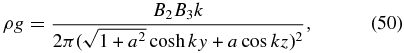
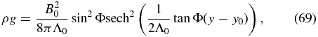
The density ρ(y, z) concentrates around the vertical plane y = 0 in a vertical series of alternating maxima and saddle points. Along y = 0, the saddle points are minima in density alternating with the maxima, having the respective values
Each of these equilibrium fluids when perturbed to evolve under the frozen-in condition moves with its flux surfaces of constant-A deforming as fluid surfaces, described by induction equation (19). The mass sandwiched between any two flux surfaces on which A = A1, A2, two constants,
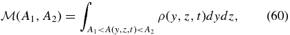
is a constant in time, where ρ(y, z, t) is the evolving density and A(y, z, t) satisfies Equation (19). To clarify our notation, with no loss of generality, we can fix A1 to define a reference flux surface. Then  is a function of a single variable A such that setting this variable A = A2, a constant, picks out the second flux surface to define the invariant total mass measured from the reference surface. We call
  the (invariant) mass function. Its derivative
  is the total mass per unit A-flux, which we refer to as mass per unit flux for brevity. We can calculate
  from the field and density in the a-family of equilibrium states. By this calculation we can attribute the two-dimensionality of the equilibrium state to the fact that the mass per unit flux varies with A when a ≠ 0, that is, flux tubes of a fixed unit axial flux are loaded with unequal total masses. The field is thus unevenly bowed by the weight varying from flux tube to flux tube. The special case of a = 0 corresponds to a uniform loading of mass for each flux tube of a fixed axial flux. These flux tubes are identical, thus compatible with equilibrium varying only in the y dimension.
The total weight averaged over a full periodicity in the z-direction given by
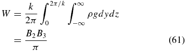
is independent of parameter a, exactly the weight W given by Equation (54) for the a = 0 1D isothermal KS slab. We recover the formula k = πk0W/B22 showing that the product of the total average weight W with the inverse isothermal scale height determines the width of the 2D slab, as well as the wavenumber of the vertical periodicity. This property characterizes the a-family of solutions in terms of their different mass functions ( ) all having the same total mass 2πW/kg per periodic cell, e.g., −∞ < y < ∞, 0 < z < 2π/k. The four states of different values of a in Figures 3 and 4 thus have the significance of having the same total mass 2πW/kg being distributed in different manners over the A-flux.
4.1.3. The 0 < a < a0 States
The mass function  and its derivatives are continuous over the simple bowed field lines for 0 < a < a0, such as shown in Figure 3. The hydrostatic density along each infinitesimally thin flux tube decreases exponentially with z, at scale height Λ0, starting from a maximum value at the lowest point of the bowed tube. This maximum value is fixed by the total mass in the tube. To address the purpose of this paper, suppose that the isothermal condition is changed by some energy process so that two contiguous thin flux tubes remain isothermal but end up with unequal temperatures along them, maintained through the absence of thermal conduction across the field. Then, in the new equilibrium, the different exponential decreases of density with z along the two tubes, at their two unequal respective scale heights, imply that the densities in the two tubes can agree at only one point along the common length of the tubes. A pressure discontinuity is unavoidable, and a discrete current must arise from the compensating discontinuity in magnetic pressure.
Suppose that we instead introduce a finite additional mass into one of the two contiguous flux tubes. For simplicity, retain the condition of a spatially uniform temperature. In the new equilibrium, the densities along the two tubes decrease exponentially with z, at the same scale height, starting from two lowest-point values different by a finite amount that we denote by Δρ0. This mass addition has rendered the mass per unit flux,  , discontinuous going across from one tube to the other. The discontinuities in the density and pressure across the tubes are proportional to Δρ0exp (− z/Λ0), strongest at the lowest point of the tubes. The heating by the resistive dissipation of the inevitable discrete current is thus expected to be most intense at the lowest points where that current is strongest.
4.1.4. The a > a0 States
The invariance of  also means that no frozen-in evolution can bring any one of these equilibrium states to another because their respective fields are topologically different. On the other hand, we may interpret the parametric sequence in Figures 3 and 4 as a quasi-static evolution of the following kind. Each of these states by its definition lies in the unbounded space but may be physically interpreted as a local idealization of a structure belonging to a much larger global structure. The open part of the field therefore may slowly have mass added or siphoned out from the global structure, under the frozen-in condition, changing the mass function
  quasi-steadily. The sequence of equilibria beginning with a = 0 and ending a = a0, in this interpretation, represents a frozen-in evolution brought about by this mass siphoning process to alter the mass function
  in a particular manner. Figure 3 shows an 0 < a < a0 state and the a = a0 state. A change of
  can result in the former evolving into the latter to produce a local concentration of mass whose weight deforms the field under equilibrium condition into a cusp point where the field intensity vanishes. The neighborhood of this point is susceptible to resistive instability resulting in the formation of a magnetic island with its X neutral point (Parker 1975; Lerche & Low 1980; Haerendel & Berger 2011). Further addition of mass into the system cannot proceed under the frozen-in condition without the X neutral point being creased into a current-sheet singularity (Parker 1994; Priest 1982). The dissipation of this current sheet relaxes the field to the continuous states exemplified by the equilibrium fields in Figure 4. In fact, the discrete-current formation is more extensive in space as we see below.
The presence of magnetic islands and separatrix lines in these states implies that the mass per unit flux,  , is not everywhere continuous over the A-flux, despite the fact that the equilibrium field and density are continuous in space. Consider the dashed separatrix in any of the two solutions in Figure 4. On the two sides of this special field line three thin flux tubes can be identified: a closed tube belonging to the magnetic island, an open tube on the upper side of the separatrix, and a third, also open, on the lower side of the separatrix. We shall refer to them as the closed, top, and bottom tubes, respectively. To compare the total masses frozen into the three flux tubes in a meaningful manner, we define the tubes to have the same (small) axial flux. Then, it is easy to verify that these three tubes contain unequal total masses as a consequence of the density being continuous in space. For example, the closed and bottom tubes are contiguous along the finite-length boundary of the magnetic island. The same exponential hydrostatic decrease with z of identical densities along the two tubes implies that the longer bottom tube must have more total mass, by a finite rather than an infinitesimal amount, in it than the closed tube. Similar reasoning applies to the infinitely long top and bottom tubes that are contiguous but not everywhere along the bottom tube.
Suppose that these three tubes adjust to a new local equilibrium under the frozen-in condition, responding to permanent changes elsewhere. For example, the particular periodic cell discussed here has changed its shape or volume permanently due to a change exterior to this cell. The evolution to new equilibrium conserves the total masses in the three flux tubes without changing the field topology. So the three tubes remain contiguous along the identifiable separatrix in the new equilibrium. In the new equilibrium, the X neutral point is likely to have been deformed into field-reversal line under the frozen-in condition. If the isothermal condition continues to apply, then the hydrostatic exponential decrease of density with z must lead to a discontinuous jump in the equilibrium density between contiguous tubes on two sides of the separatrix line, since their respective masses are conserved but their tube volumes have changed. The separatrix must then carry a discrete current to account for a magnetic-pressure jump to compensate the inevitable pressure jump across the separatrix.
Another instructive illustration of this effect is given by the following thought experiment. Take one of the fields in Figure 4 as an initial state but load it with an everywhere continuous mass per unit flux,  . This initial state is not in equilibrium, and we let it evolve under the frozen-in and isothermal conditions to equilibrium. The separatrix and the three thin flux tubes on its two sides can never have continuous density across the separatrix in that equilibrium. This follows from the overconstraint of the density having to decrease with z with a fixed scale height, and the flux tubes conserving their total masses have no control over their respective tube volumes in the equilibrium state.
We should remind ourselves that by the assumption of a uniform temperature we have removed powerful energy-transport processes such as the one considered in Paper I. In our analysis, we use the pure isothermal equilibrium to show how readily discrete currents can form when this simple state is perturbed. If we subject each of the flux tubes of fluid in this equilibrium to the steady energy transport in Paper I, involving radiative loss, heating, and field-aligned thermal conduction, for example, it is clearly conceivable that this transport is greatly influenced not just by the total mass in a flux tube, as shown in Paper I, but also by its geometric shape. In Figure 4, energy transport takes on significantly different forms depending on whether the flux tube is closed or open. The thermal collapse of a fraction of the total mass in a flux tube followed by its resistive drainage across the field, say, from the magnetic island to the external open field, has many dynamical consequences in terms of sinking overloaded flux tubes, a magnetic island made buoyant by its loss of mass, and, of course, the formation and dissipation of new discrete currents. Our static analysis has its limit but is sufficient for pointing out these interesting effects by inference, leaving the interesting and unambiguous dynamical effects for future time-dependent studies.
4.1.5. Endless Intermittently Resistive Evolution
Although the a-family of isothermal solutions is artificial from the physical point of view, their properties described above point to the following general hydromagnetic process quite relevant to the solar prominence. The resistive dissipation of a discrete current flowing in an entire flux surface across which the density is discontinuous delivers a finite, as opposed to an infinitesimal, mass from one side to the other. This dissipation enabling the field to diffuse resistively across the fluid is time dependent and sensitive to the precise nature of the dissipative process. Therefore, the finite amount of mass so transported across the field is effectively a random quantity, being dependent on the nature and course of events in the dissipative process. As soon as the extreme field gradients have been dissipated away, the frozen-in condition is restored as an excellent approximation. Because the mass transported across from one flux bundle to another is finite and uncontrolled, it follows that such a process cannot, in general, either produce a mass per unit flux everywhere continuous across the magnetic flux or be piecewise continuous to be just right to ensure that where there are X neutral points in the field, the equilibrium density is everywhere continuous.
This conclusion is simplest to see if we avoid the complication of magnetic reconnection and deal with just resistive diffusion of field across a fluid surface. Consider two closed flux tubes in one of the magnetic islands in Figure 4 of the same unit axial flux and contiguous along their entire lengths. Let one tube have a total mass a finite amount larger than the total mass of the other. Between them in equilibrium is a discrete current required for the balance of their jump in fluid pressure. The dissipation of that discrete current brings about a resistive diffusion of the magnetic flux across the fluid boundary separating the fluid in the original two flux tubes. In relative terms, the original two flux tubes can be identified in the diffused field, and we may then say that they have exchanged mass between them. Now, this process, whatever its physical resistive nature, is not constrained such that just the right finite amount of mass would have passed to equalize the total masses of the two flux tubes in the final state. That is, although a finite amount of mass has passed between the two flux tubes, this amount is uncontrolled. Therefore, after the dissipation, the new total masses in the two flux tubes, in general, would still have a finite difference between them. With the extreme field gradients removed resistively, the frozen-in condition is restored. This means that the field's discontinuous mass per unit flux,  , is invariant in the evolution that follows. The system is thus set up for the next in a never-ending sequence of bouts of resistive dissipation. Once started, the formation and dissipation of discrete currents repeat intermittently in this manner.
The inevitability of discrete-current formation is topological, that is, it has to do with anisotropy in thermal conduction and the anisotropic Lorentz force. This inevitability is separate from how energetic the discrete currents would be in a given bout of dissipation, the latter depending on the free energy available (Janse & Low 2010). In the case of the quiescent prominence, an important source of energy for this endless intermittently resistive evolution is the gravitational potential energy of the system. In a complex 3D field, every resistive event opens new paths in the local reconnected field for the fluid to flow to lower gravitational potential energy, while a reconfigured flux tube drained of some of its fluid would rise by magnetic buoyancy (Berger et al. 2010). The tortuous process ends only when all the mass has drained out of the magnetic field, which we are assuming to have somehow gotten into the atmosphere.
So, if the system is driven with a continual injection of mass and magnetic flux into the system, then the dissipation can conceivably be sustained. The accumulation of buoyant magnetic flux and helicity can explain the large coronal cavity that contains the quiescent prominence (Priest et al. 1989; Low 1996, 2001; Zhang & Low 2005; Low & Hundhausen 1995; Schmit et al. 2009; Fan & Gibson 2006, 2007; Schmit & Gibson 2011; Fuller et al. 2008; Dove et al. 2011; Gibson & Fan 2006; Gibson et al. 2010). In this picture the ultimate source of energy is magnetic, providing the heating of plasma to be injected into the cavity to be condensed into the prominence. We have only provided an elementary theoretical analysis, but this analysis suggests some rudiments for the magneto-thermal convection proposed by Berger et al. (2011) to explain the phenomenon of the quiescent prominence with the unprecedented observations from Hinode/SOT and SDO/AIA. The dissipation puts a limit of how much mass may be retained in the system on a long quasi-steady timescale, determined by the mass injection and drainage rates. Liu et al. (2012) reported the first observation of such a quasi-steady balance in a prominence made with SDO/AIA. In this event, the drainage rate is significant to the level of the prominence having drained an estimated total mass of about 1015 g, of the order of the magnitude of a CME mass, in a day while retaining an estimated, quasi-steady total mass in the prominence of an order of magnitude smaller.
These prominence observations are the motivation of our theoretical development in this paper. To complete this development, we present two explicit families of solutions describing inevitable discrete currents arising from discontinuity in mass per unit flux, as well as the discontinuity of a temperature that is isothermal on but varying across magnetic flux surfaces.
4.2. Equilibrium with Discontinuous Total Mass per Unit Flux
There is a family of analytic solutions to the isothermal Grad–Shrafanov equation (35) especially suited for illustrating 2D equilibrium states in which the mass per unit flux,  , is a discontinuous function (Low & Manchester 2000; Manchester & Low 2000). These solutions satisfy the Grad–Shrafanov equation (35) with p0(A) being a discontinuous function of A.
Prescribe the constant-A field lines to be contours of constant ϕ(y, z), where

This simply means that A(y, z) = A(ϕ) and Equation (35) reduces to the following ordinary differential equations:
relating A(ϕ), Q(ϕ), and p0(ϕ). Figure 5 displays the contours of constant ϕ(y, z), comprising horizontally periodic cells of U-shaped field lines resting on a bed of horizontally oriented field lines. The field line ϕ(y, z) = 1 separates the latter set of lines from the periodic cells, running up to z → ∞ and back as the boundary of each successive cell. To build an equilibrium of this family of solutions, we may prescribe p0(ϕ) arbitrarily, that is, specifying the isothermal pressure distribution p(y, z) = p0[ϕ(y, z)]exp (− k0z). This specification is equivalent to prescribing  on the field lines of a fixed shape. Equations (63) and (64) then determine A(ϕ) and Q(ϕ) in terms of the prescribed p0(ϕ) and yield the equilibrium magnetic field given by Equation (8). Note that in Figure 5 the upper periodic U-shape fields can be loaded with vertically elongated fluids with their lower ends terminating at a height beneath which the field is of a contrastingly different topology, the latter suggestive of the observed quasi-steady macroscopic voids at the base of prominences (Berger et al. 2010, 2011).
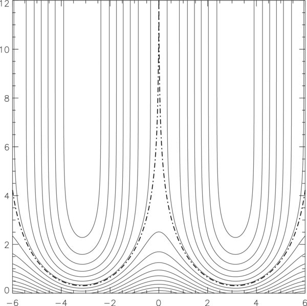
Figure 5. Field lines of constant-ϕ(y, z), defined by Equation (62), projected on the plane with k0y on the abscissa and k0z on the ordinate. The field is periodic in y, everywhere vertical in the z → ∞ region and morphing into a horizontal wavy field in the z → −∞ region, separated by the (dashed) separatrix field line ϕ = 1.
Download figure:
Standard image High-resolution imageIn the original studies (Low & Manchester 2000; Manchester & Low 2000), interest was concentrated on A(ϕ) having an everywhere continuous derivative, so that both the field and plasma are everywhere continuous in space. This family of solutions includes the case of p0(ϕ) prescribed as a discontinuous function corresponding to a discontinuous  . Suppose that p0(ϕ) is discontinuous across a flux surface ϕ = ϕ1, a constant; then Equations (63) and (64) demand that both (dA/dϕ)2 and Q2 are also discontinuous across ϕ = ϕ1. The latter implies that the magnetic pressure given by
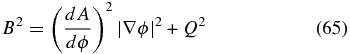
is discontinuous across ϕ = ϕ1. Independent of whether or not p0(ϕ) is continuous, the total pressure is
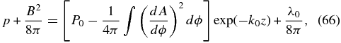
derived from the force-balance equation (4). Thus, we are assured that the discontinuities in fluid pressure and magnetic pressures in the above construction automatically satisfy the continuity of the total pressure as a requirement for the surface of discontinuity dA/dϕ to be in force balance. We leave the reader to explore the properties of this family of solutions.
The sets of continuous and discontinuous equilibrium solutions are infinite, spanned by all forms of  , all sharing the same field lines displayed in Figure 5. Clearly, the set of continuous equilibria is a subset of measure zero of the set of all realizable equilibria.
4.3. Discontinuous Tangential Fluid Displacement at a Magnetic Flux Surface
The nonlinear Grad–Shrafanov equation (21) for a prescribed temperature θ(A), constant on each flux surface but allowed to be of different values on different flux surfaces, is generally analytically intractable and non-trivial to solve numerically. We turn to the 2D extension of the 1D isothermal KS slab, in an entirely different geometry, by Low & Petrie (2005) for an explicit illustration of inevitable discrete currents arising from distributions of temperature and total frozen-in mass that are discontinuous across magnetic flux surfaces.
The 1D KS slab solution described by Equations (51)–(53) has three free parameters, (B1, B2, B3). Let us set B1 = 0, limiting our attention to fields that lie in the y − z plane, and redefine B2 = B0cos Φ, 2B3 = B0sin Φ in terms of two equivalent free parameters B0 and Φ. With k = k0B3/B2 = (1/2Λ0)tan Φ, we obtain the solution
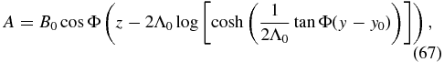


where we have introduced a constant translation displacement y0 in the y-direction with no loss of generality. The weight defined by Equation (54) is now expressed as
We have done no more than rewrite the 1D solution in another equivalent form.
What is interesting is that if we now formally take B0 a constant in space but let Φ, Λ0, y0 be arbitrary functions of x, we still have a solution to the force-balance equation (4), which, for our purpose here, we rewrite as
First, the variation with x introduced retains the solenoidal condition on B. Direct evaluation shows that p + B2/8π = B20/8π, uniform in 3D space, and (B · ∇)B gives only a vertical component that balances the weight ρg exactly. Thus, the force balance is satisfied for all prescribed Φ(x), Λ0(x), and y0(x). This was shown by Low & Petrie (2005), except that they had not realized that the scale height Λ0, too, may vary freely with x, allowing for a corresponding temperature T = T0(x), for a solution of this kind. Finally, an arbitrary function y0(x) displaces the solutions on different x-planes arbitrarily, creating quite complex structures (Low & Petrie 2005; Petrie & Low 2005).
Each of these 2D equilibrium states is a bowed magnetic field lying in planes of constant x, wherein By = B0cos Φ(x) and the temperature T = T0(x) are uniform, supporting the weight W(x), given by Equation (71), frozen into the field. The 1D KS slab corresponds to Φ, Λ0, and y0 being the same constants on all x-planes as magnetic flux surfaces. Arbitrary loadings of weight W(x) and different temperatures T0(x) on these flux surfaces are admissible, giving rise to field patterns varying across the flux surfaces in terms of the sag of the bowed field, density, and field intensity as functions of x. The original study of Low & Petrie (2005) was interested in continuous variations.
The study in the present paper introduces a new interest, namely, the equilibrium states of fields endowed by their resistive past with a distribution of total mass in magnetic flux tubes that is not continuous across flux tube boundaries. Once the discontinuous distribution has been acquired and the frozen-in condition restored as an excellent approximation, the field will relax into an equilibrium state that is expected to be discontinuous in fluid and field properties across the flux surfaces. Taking the final equilibrium state to be isothermal on flux surfaces as a simplifying assumption, we have two independent origins for the discontinuity, one being the different constant temperatures on isothermal flux surfaces and the other being the different total mass per unit magnetic flux in flux tubes on either side of a flux surface. We present examples of these two properties.
Figure 1 shows three solutions of different total weight W at the same temperature T0 and scale height Λ0. A continuous variation with x through these three solutions gives an everywhere continuous equilibrium state varying with x and y. A prescription of W(x) that jumps discontinuously from two different states in Figure 1 across a flux surface x = x0, a constant, would have the superimposed field lines shown on the left in Figure 6. Everywhere on x = x0 we see a discontinuous B across this flux surface, a magnetic tangential discontinuity carrying a discrete current flowing in that flux surface. Note that independent of the choice of W(x) and T0(x), the total pressure p + B2/8π = B20/8π is uniform in space and therefore continuous across x = x0, satisfying the condition for x = x0 to be in force balance. In this case, not only is the direction of B discontinuous across x = x0, but so is B2, from which follows that the density and pressure are both discontinuous across that surface. As long as electrical conductivity is perfect, this discontinuous equilibrium is admissible as a steady state, but our interest in obtaining this solution is to make the point that electrical conductivity in a real solar plasma is extremely high but finite, so that the formation of this singularity leads to resistive dissipation and magnetic reconnection.
Figure 6. Magnetic flux surface x = x0 across which the equilibrium field B(x, y), given by Equation (68), is discontinuous in both field intensity and direction such that the total pressure is continuous to ensure force balance everywhere on x = x0. Shown are two sets of field lines, the thick lines on one side overlaid on the thin lines on the other side of x = x0 for each of two exact solutions described in the text. In the left panel the two sets of field lines for a solution have the same isothermal temperature but different total masses loaded per unit magnetic flux; see Figure 1. The two sets of field lines in y → ±∞ have different constant gradients, and the discrete current flowing in x = x0 is everywhere intense. In the right panel the two sets of field lines for the other solution have different isothermal temperatures but the same total mass loaded per unit magnetic flux; see Figure 2. The two sets of field lines in y → ±∞ have the same constant gradient, and the discrete current flowing in x = x0 is intense only in the neighborhood of y = 0 but vanishes in y → ±∞.
Download figure:
Standard image High-resolution image
As pointed out by Low & Petrie (2005), the far fields on different x-planes have different inclinations to the horizontal because the sets of field lines in the x-planes are loaded with different weight W. It is simple to show that B in the far region y → ±∞, ρ → 0 and the sheared field is in a force-free state ∇ × B = α(x)B with α = ±dΦ(x)/dx. This field feeds into or takes out field-aligned currents from both sides of the 2D slab in order to regulate the cross-field current flowing in the x-direction within the slab. This current density distribution self-consistently accounts for just the right amount of cross-field current in the slab so that Lorentz force is nonzero and exactly supports the weight of the slab in the different x-planes.
The solution on the right in Figure 6 corresponds to the three solutions in Figure 2 with different temperature T0 on different x-planes but the same weight W. Using these solutions to construct a 2D solution varying with x and y, let us suppose that T = T0(x) jumps discontinuously from one state to another in Figure 2 across x = x0. Then, the fields on the two sides of x = x0 seen projected on x = x0 are different, as shown on the right in Figure 6, producing a discrete current flowing on that surface. Again, the field, density, and pressure are all discontinuous across x = x0. Since the weight W is the same for all x, that is, Φ is a constant, it follows that α = 0, and the far field in y → ±∞ does not vary with x, evident in the right panel of Figure 6. The current density generating the x-varying supporting Lorentz force in the 2D slab is not strictly in the x-direction, meandering around in the x−y plane but confined around the central plane y = 0 of the slab. Again, the discrete current in x = x0 must dissipate at the small resistivity of a real plasma, leading to reconnection and changes in mass distribution over the magnetic flux.
5. SUMMARY AND CONCLUSION
Our theoretical investigation, in Papers I and II here, provides a basis to hypothesize that the ever-restless dynamical state of the interior of a certain class of quiescent prominences observed with Hinode/SOT and SDO/AIA has its origin in the spontaneous formation and resistive dissipation of discrete currents under the condition of high electrical conductivity. The long-lived polar-crown prominences, prior to eruption, exemplify this class; see the discussions in Paper I.
The formation and resistive dissipation of discrete currents are an endless, intermittent process first conceived by Parker (1972, 1994) to explain the magnetic heating of solar and stellar coronae. The version of this theory we pursue here centers on the highly anisotropic thermal conductivity in the corona. An examination of the weak cross-field thermal and resistive diffusivities in a magnetized fully ionized gas described by Spitzer (1962) indicates that the former is by far the weaker effect in the low-β corona and prominences. In the idealization of neglecting cross-field thermal conduction, the temperature is allowed to be discontinuous across magnetic flux surfaces, naturally producing finite jumps in fluid pressure across these surfaces. In an evolution to equilibrium under the frozen-in condition, the field readily becomes tangentially discontinuous across each of these surfaces, producing a discrete current and a magnetic-pressure jump across the surface to balance the fluid-pressure jump. In a real plasma of an extremely high but finite electrical conductivity, this evolution proceeds with a steepening of field gradients during the time the frozen-in approximation is good, only to result in such extreme gradients that dissipation at the small resistivity of the fluid becomes significant. The resistive removal of the strong gradients then restores the frozen-in condition only to evolve to the next bout of gradient steepening and resistive dissipation.
A comment is in order on the theoretical approach in our treatment of this intrinsically time-dependent process. To relate this process to the observed corona requires powerful numerical simulations in multi-dimensional space and a multi-fluid description for physical completeness (Gilbert et al. 2002, 2007; Greenfield et al. 2011). Considering that the process is not well understood, this series of papers aims at its basic effects in the one-fluid description. To avoid having to solve a time-dependent problem, we have treated the equivalent static problem by examining a static equilibrium as an end-state of a hydromagnetic evolution under the frozen-in condition. The connection between an equilibrium state of interest with the possible evolutions ending in this state can be made. This is done by explicitly imposing a specific field topology and a specific mass function, both invariant under the frozen-in condition, to constrain the equilibrium state.
To illustrate the point, the Grad–Shafranov PDE (35) describing an isothermal equilibrium state has the free functions p0(A) and Q(A). If we are generating a state without further constraints, these free functions may be prescribed a priori and we have the classical problem posed by an elliptic PDE. When the invariants of a frozen-in evolution are imposed on an equilibrium state of interest, the functions p0(A) and Q(A) are to be solved as unknowns together with A(y, z). We prescribe the mass function  , a frozen-in invariant, instead of p0(A); the two are related by Equation (60). The function
  is well defined independent of whether the system is in equilibrium, whereas p0(A) is meaningful only in an equilibrium state. Similarly, Q(A) is an unknown and must be subject to an integral equation relating it for all time to the invariant amount of flux in the x-direction lying between any two constant-A flux surfaces, in perfect analogy with Equation (60). In this formulation of the problem, the functions p0(A) and Q(A) are unknowns governed by integral equations to be coupled to the Grad–Shafranov PDE (35). The inevitable discontinuous solutions we must admit come from the structure of this system of integro-PDEs.
This static problem is just as formidable as its equivalent time-dependent problem, so we probe for physical properties by analyzing the three families of solutions presented. In general terms, the inevitable discrete currents can arise in four independent ways. The first is basically a thermal collapse, treated in Paper I with a tractable 1D process in the 1D KS slab. The discrete current comes from a discontinuity in the bowed field to generate a discrete Lorentz force to support the thermally collapsed mass sheet. The other three ways of spontaneously forming discrete currents are multi-dimensional effects. The one of immediate interest arises from the temperature being discontinuous across a flux surface because the cross-field thermal conductivity is completely suppressed. The jump in fluid pressure implied by the temperature discontinuity requires a discrete current to create a compensating cross-field jump in magnetic pressure. Another way for producing a pressure jump comes from a discontinuous loading of mass in the field under the frozen-in condition, that is, the invariant function  is discontinuous. These two ways of spontaneous formation of discrete currents in equilibrium states are neatly illustrated by the analytical solutions presented in Section 3. Finally, the fourth way for a discrete current to arise is the general formation of tangential discontinuities in the field inevitable if a complex 3D field topology is to be preserved as it relaxes into equilibrium under the frozen-in condition, with or without the presence of fluid pressure and gravity (Parker 1994). The above classification is helpful for sorting out the basic effects, but in a complex magnetic field in the corona, all these effects are irrepressible and coupled to one another.
Among the properties we have illustrated, one stands out for emphasis. Although we could only construct extremely idealized equilibrium solutions, they are sufficient for pointing out a general property. When a discrete current dissipates resistively in the presence of a finite, as opposed to an infinitesimal, jump in density across it, a finite amount of mass is transferred across a flux surface. That finite amount is uncontrolled, and it follows that no single cross-field transfer of mass can preserve an everywhere continuous  or create an everywhere continuous
  from an initially discontinuous one. This leads to the physical picture that once initiated, the bouts of spontaneous formation and resistive dissipation of discrete currents must repeat intermittently forever until the free energy runs out (Janse & Low 2010). The origin of this property is ultimately high electrical conductivity. It is high electrical conductivity that creates such high magnetic gradients that resistivity, small but not zero, becomes significant. In this manner, despite the high magnetic Reynolds numbers in the quiescent prominence, the flow has an intermittent component that is more resistive than these numbers would have suggested. The prominence fields are strong, in the range of 5–60 G (Casini et al. 2003; Leroy 1989; Lopez Ariste & Casini 2003; Trujillo Bueno et al. 2002). Even though the plasma-β is small, the field in our physical picture must also actively evolve with the fluid. As we have pointed out in Section 4.1.5, this process can explain the significant drainage of prominence mass as observed by Liu et al. (2012), in particular, and may be relevant to advancing the proposal by Berger et al. (2011) that the quiescent prominence is a magneto-thermal convective process. The rudimentary theoretical ideas we have described provide motivation for further investigation using high-power numerical simulation.
We thank Yuhong Fan for a helpful review. The National Center for Atmospheric Research is sponsored by the National Science Foundation. T.E.B. was supported by the Solar-B FPP contract NNM07AA01C at Lockheed Martin. W.L. is supported by NASA SDO/AIA contract NNG04EA00C.