


ABSTRACT
Since 2008 December, the Interstellar Boundary Explorer (IBEX) has been making detailed observations of neutrals from the boundaries of the heliosphere using two neutral atom cameras with overlapping energy ranges. The unexpected, yet defining feature discovered by IBEX is a Ribbon that extends over the energy range from about 0.2 to 6 keV. This Ribbon is superposed on a more uniform, globally distributed heliospheric neutral population. With some important exceptions, the focus of early IBEX studies has been on neutral atoms with energies greater than ∼0.5 keV. With nearly three years of science observations, enough low-energy neutral atom measurements have been accumulated to extend IBEX observations to energies less than ∼0.5 keV. Using the energy overlap of the sensors to identify and remove backgrounds, energy spectra over the entire IBEX energy range are produced. However, contributions by interstellar neutrals to the energy spectrum below 0.2 keV may not be completely removed. Compared with spectra at higher energies, neutral atom spectra at lower energies do not vary much from location to location in the sky, including in the direction of the IBEX Ribbon. Neutral fluxes are used to show that low energy ions contribute approximately the same thermal pressure as higher energy ions in the heliosheath. However, contributions to the dynamic pressure are very high unless there is, for example, turbulence in the heliosheath with fluctuations of the order of 50–100 km s−1.
Export citation and abstract BibTeX RIS
1. INTRODUCTION
In 2008 October, the Interstellar Boundary Explorer (IBEX) mission (McComas et al. 2009b) was launched into Earth's orbit with the objective of discovering the global interaction between the solar wind and the interstellar medium. Science operations began in late 2008 December. The science payload on this small explorer mission consists of two high-sensitivity, single-pixel, neutral atom cameras, a star sensor, and an ion background monitor. The two neutral atom cameras have overlapping energy ranges; the IBEX-Lo sensor covers the energy range from 0.01 to 2 keV and the IBEX-Hi sensor covers the energy range from 0.3 to 6 keV. Both sensors have an approximately 7° × 7° field of view and a view perpendicular to the spin axis of the spacecraft. Over a spin (and during an entire orbit), the sensors sample a 7° × 360° swath in the sky. The spin axis is directed approximately toward the Sun and, up until the orbit was changed (in 2011 June, see McComas et al. 2011a), spin axis re-pointing occurred once every 7–8 day orbit. Re-pointing keeps the solar array directed toward the Sun and allows adjacent swaths to be filled in to form a complete sky map in six months. The sky maps are numbered starting from the first six-month observation period in late 2008 December through 2009 June. Since the start of science operations, the cameras have completed six sky maps, and a seventh sky map is currently being accumulated.
Two sensors are needed because different neutral atom detection techniques are required to cover the full energy range (see Wurz 2000; Fuselier et al. 2009b; Funsten et al. 2009a). Both sensors convert neutrals to ions and subsequently accelerate and deflect these ions into low-background, triple coincidence detector systems. IBEX-Lo uses a conversion surface to convert neutrals to negative ions while IBEX-Hi uses ultra-thin carbon foils to convert neutrals to positive ions. Because the sensors have different neutral to ion conversion efficiencies and different sizes, they have different overall sensitivities; IBEX-Hi is approximately 10 times more sensitive than IBEX-Lo at the overlapping energy of ∼1 keV. Since the heliospheric neutral atom signal is very weak and the two sensors respond differently to a variety of potential backgrounds (e.g., UV, solar wind electrons and ions, energetic ions from the near-Earth environment, neutrals from Earth's magnetosphere), two independent neutral atom measurements provide strong confirmation of the first observations of the interaction between the solar wind and interstellar medium.
IBEX sensors are susceptible to a variety of backgrounds that change depending on the location of the spacecraft within near-Earth plasma regions. Prior to launch, an extensive study of potential background sources was done (Wurz et al. 2009). These backgrounds include the solar wind, energetic ions from the near-Earth environment, energetic electrons, and an internal background unique to IBEX-Lo. The backgrounds affect IBEX-Hi and IBEX-Lo differently and are removed in the process of creating the sky maps. In addition to these backgrounds, several nonheliospheric sources of energetic neutral atoms are important. They include the Moon (McComas et al. 2009a; Rodríguez et al. 2012), Earth's magnetosphere and magnetotail (Fuselier et al. 2010; Petrinec et al. 2011; McComas et al. 2011b), and interstellar neutral atoms (ISNs; Möbius et al. 2009). Of these nonheliospheric sources and backgrounds, the two of particular interest in this present study are the ISN source and the IBEX-Lo internal background.
Interstellar neutrals: IBEX-Lo measures neutrals from 0.01 to 2 keV by first converting the neutrals to negative ions on a conversion surface (Fuselier et al. 2009b). In January and February every year (time periods in odd number sky maps that extend from approximately December to June), IBEX-Lo observes ISNs in the energy range from 0.01 to ∼0.6 keV (Möbius et al. 2009). ISNs that are directly converted to negative ions on the IBEX-Lo conversion surface consist of mainly hydrogen and oxygen. Oxygen is separated from hydrogen by the IBEX-Lo time-of-flight subsystem and is eliminated from the analysis. In addition, ISN helium, hydrogen, and oxygen (and other, heavy ISN species) sputter hydrogen and oxygen negative ions off the conversion surface (e.g., Saul et al. 2012). Of these sputtered products, hydrogen sputtered by ISN helium is the most significant and is several orders of magnitude higher than negative ions directly converted from heliospheric hydrogen neutrals. For this present study, these fluxes represent a significant nonheliospheric source that makes analysis of heliospheric neutrals in some parts of odd numbered sky maps at lower energies very difficult. The effects of the ISN signal in the sky maps are discussed in detail below.
IBEX-Lo internal background: IBEX-Lo has an internal background that is unique to its neutral detection technique. Any ion or neutral with sufficient energy incident on the conversion surface has a finite probability of "sputtering" a negative ion off the conversion surface. Here, the term sputtering is used to encompass all negative ion production by knock-off from the conversion surface, from very low energies up to the energy of the incident particle. Any particle flux with sufficient energy that impacts the conversion surface produces this sputtered background, including ISN helium (a major source of sputtering in odd numbered sky maps), energetic ions from the near-Earth environment, neutrals from the near-Earth environment, and even heliospheric neutrals. Sputtered contributions are removed from analysis by using a combination of IBEX-Lo laboratory calibration results and in-flight flux measurements from IBEX-Hi.
All backgrounds and nonheliospheric sources have some type of mitigation that allows detection of weak heliospheric neutral fluxes in both sensors. Initial science results from the mission were published after the first sky map was completed in 2009 (McComas et al. 2009b). The unexpected, yet defining feature in this first sky map (and in subsequent maps as well) was a Ribbon of neutral fluxes oriented approximately perpendicular to an independent estimate of the direction of the interstellar magnetic field (McComas et al. 2009a; Schwadron et al. 2009; Funsten et al. 2009b). This Ribbon extends over the energy range from about 0.2 keV to 6 keV and is superposed on a more uniform, globally distributed flux (McComas et al. 2009c; Fuselier et al. 2009a; Schwadron et al. 2011).
With some important exceptions (e.g., McComas et al. 2009b; Fuselier et al. 2009a), most of the initial and subsequent results from the mission focus on the IBEX-Hi energy range from about 0.5 to 6 keV. For the globally distributed flux, the dominant parent ion source for neutrals in the energy range above 1 keV is likely ions that were originally picked up in the heliosphere before the solar wind encountered the termination shock (e.g., Gruntman et al. 2001; Prested et al. 2008; Gloeckler & Fisk 2010). The neutrals are produced by ionization (pick up) of interstellar neutrals by the solar wind in the heliosphere, transport of these ions across the termination shock with the solar wind, charge exchange in the heliosheath downstream of the termination shock, and return of these neutrals back to the inner heliosphere. The solar wind velocity in the heliosphere is relatively high (400–800 km s−1 or corresponding to energies >1 keV). Therefore, these heliospheric neutrals exhibit characteristic energies of their parent ions and have energies greater than 1 keV.
Neutrals from this parent ion population have been the focus of most IBEX studies because of background issues in the lowest energy channel of IBEX-Hi and because of counting statistics and ISN background issues in IBEX-Lo. At energies below ∼1 keV, contributions to heliospheric neutral fluxes from two additional parent ion populations may become significant. From about 0.2 to 1 keV, a potentially important parent ion population for neutrals observed by IBEX may be heliosheath pick-up ions (e.g., Chalov et al. 2003; Gloeckler & Fisk 2010). These pick-up ions are produced in a similar fashion as pick-up ions in the pretermination shock solar wind, except that now interstellar neutrals are ionized in the inner heliosheath. Across the termination shock, the solar wind slows to roughly 100 km s−1, as measured at the Voyager 2 spacecraft in the heliosheath (Richardson & Wang 2011). Therefore, heliosheath pick-up ions and the resulting neutrals have lower energies (below ∼0.7 keV). Finally, below about 0.2 keV, the heliosheath solar wind (the solar wind beyond the termination shock) may be a significant contributor of neutrals observed by IBEX.
With the accumulation of six complete sky maps and a better understanding of potential background contamination of the heliospheric signal, a more detailed study of the heliospheric neutrals below 0.5 keV is possible. This paper presents observations of neutral atoms from 0.01 to 6 keV from IBEX-Lo and IBEX-Hi from the first three sky maps, with particular emphasis on the comparison between results above 0.5 keV and new results below 0.5 keV. The focus is on energy spectra from several selected regions in the heliosphere, including directions of the Voyager spacecraft, the Nose (the upwind direction), and a part of the Ribbon at southern latitudes. Below 0.5 keV, heliospheric neutral flux spectra are very uniform, exhibiting a similar spectral index in all directions investigated. These spectra are used to derive the ion pressure multiplied by the heliosheath radial thickness over the entire IBEX energy range and quantify the contributions from lower energy heliosheath ions to this pressure multiplied by radial thickness.
In Section 2, sky maps for energies below 0.5 keV are introduced and specific regions in the sky are selected. In Section 3, energy spectra from specific regions in the sky are compared. In Section 4, energy spectra are used to compute pressures in the outer heliosphere. Section 5 contains conclusions, and the Appendix discusses heliospheric observations made when IBEX was in Earth's magnetospheric lobes.
2. SKY MAPS AND SELECTED PIXELS
Sky maps are created by combining flux versus spin angle from individual orbits. For each orbit, the selection of good heliospheric viewing starts with the removal of times and angles when the sensors view the Moon and Earth's magnetosphere. Further culling of the data to remove intervals when backgrounds are present is done differently for IBEX-Lo and IBEX-Hi because backgrounds are different for the two sensors. For IBEX-Lo, good heliospheric viewing intervals are selected by separately binning data from the highest two energy channels over 180° and selecting only those intervals when there are 3 counts or less over a 96 second interval in both energy channels. This maximum count rate was determined by comparing the IBEX-Lo count rate with the IBEX ion background monitor during the first year of operations (energetic ions are the single largest contributor to background in IBEX-Lo). The selected intervals are used for all IBEX-Lo energy channels. For IBEX-Hi, good heliospheric viewing intervals are selected for each energy step individually. They are determined by summing counts over all spin angles and identifying a minimum count rate during each orbit. Only intervals when count rates are at the minimum (for that particular energy) are retained.
Figure 1 shows an IBEX-Lo sky map at 0.439 keV that was created by combining IBEX-Lo maps 1 and 3. The sky map is a Mollweide projection nearly in ecliptic coordinates (the center of the projection is the Nose direction, which is at an ecliptic latitude of about 5º). The nominal direction of the heliospheric tail is at the left and right edges of the map. Fluxes are in the spacecraft frame at the center passband of IBEX-Lo energy channel 6 (0.439 keV center energy).

Figure 1. IBEX-Lo sky map (Mollweide projection) at 0.439 keV created by combining maps 1 and 3. The Ribbon extends across the center of the map and is about 1.5–2 times higher than surrounding fluxes. It snakes between the directions to the two Voyager spacecraft. Background features evident in the map include high fluxes from Earth's magnetosphere surrounding the region where IBEX views through the magnetosphere (the black region from 130º to 160º longitude) and high fluxes at 330º longitude from early in the mission. Locations of the four "pixels" used in the study are shown in orange.
Download figure:
Standard image High-resolution imageThe Ribbon extends across the center of the map from latitude, longitude of +45º, 330º to −20º, 180º and snakes between the directions of the two Voyager spacecraft. Neutral fluxes in the Ribbon are about 1.5–2 times higher than surrounding fluxes. Fluxes in the nominal heliotail region (at the left and right edges of the map) and the aberrated heliotail (Schwadron et al. 2011) (centered at latitude, longitude −5º, 15º) are 3–4 times lower than fluxes from the Nose and Ribbon regions. Background features evident in the map include high fluxes from Earth's magnetosphere surrounding the region where IBEX views through the magnetosphere (the black region from 130º to 160º longitude) and high fluxes at 330º longitude from early in the mission when there was a high electron background in the IBEX-Lo time-of-flight system. (This background was removed by setting a higher threshold for the time of flight of incoming particles after orbit 12, and thus it does not affect subsequent orbits.)
Four large "pixels" are selected to investigate ENA energy spectra. These pixels are shown in Figure 1. The centers of these pixels are the directions toward the two Voyager spacecraft (V1 at 35º, 255º, V2 at −32º, 289º), the Nose (at 5º, 255º), and the Ribbon at southern latitudes (−20º, 255º). Pixel centers are the same as those used by McComas et al. (2009c), except for the Ribbon pixel, although pixel sizes are somewhat different. The Voyager 1, Nose, and Ribbon pixels were chosen so that a corresponding set of pixels from map 2 (when the spacecraft was in Earth's magnetosphere) could be compared to the ones from the combined maps 1+3 (when the spacecraft was in the solar wind). This comparison is discussed in Section 3 in connection with the energy spectra. The Appendix contains a complementary detailed comparison in connection with the observations made from Earth's magnetospheric lobes.
Figure 2 shows the difficulty encountered when studying heliospheric neutral fluxes and searching for Ribbon signatures in the lower energy channels in IBEX-Lo (below 0.2 keV). This figure shows the corresponding combined maps 1+3 for IBEX-Lo energy step 4, centered at 0.11 keV. Unlike the map at 0.439 keV in Figure 1, this map at 0.11 keV is dominated by very intense neutral fluxes centered approximately on the ecliptic from longitude 180º to 270º. These are hydrogen (negative ions) created by sputtering off the IBEX-Lo conversion surface by ISN helium (Möbius et al. 2009, 2012). Although there is some evidence for enhanced flux at lower southern latitudes (near the location of the Ribbon pixel) when compared to higher northern latitudes (above the ISN background), it is difficult to determine if the Ribbon exists at this energy from these observations. In terms of contamination from ISN signal, the Voyager 2 pixel is the least contaminated since it is furthest away, followed by the Voyager 1 pixel, then the Ribbon pixel and finally, the Nose pixel is the most contaminated. Contamination occurs in all four of the lowest energy channels of IBEX-Lo. In terms of count rates, the contamination is approximately the same for the three lowest channels and the count rate in the fourth energy channel (i.e., the energy channel in Figure 2) is approximately half the count rate of the three lowest channels. Since the geometric factor of the sensor decreases approximately linearly with decreasing energy, nearly equal count rates produce an apparent power-law flux distribution.

Figure 2. IBEX-Lo sky map (Mollweide projection) at 0.11 keV created by combining maps 1 and 3. The format is the same as in Figure 1. The dominant feature in this map is not the Ribbon, rather it is a broad region of intense fluxes from −100° to −180° longitude that are created by sputtering off the IBEX-Lo conversion surface by ISN helium. In terms of contamination from ISN related signal, the Voyager 2 pixel is the least contaminated since it is furthest away from the intense fluxes, followed by the Voyager 1 pixel, then the Ribbon pixel and finally, the Nose pixel is the most contaminated.
Download figure:
Standard image High-resolution imageIn principle, sputtered hydrogen from ISN helium (and directly converted ISN hydrogen) can be removed from the lower energy channels using data from map 2 (from 2009 July through December) when the ISN helium flux is low and the helium energy is below the minimum energy of IBEX-Lo. Unfortunately, for even numbered maps like map 2, the spacecraft is mainly in Earth's magnetosphere, and there is apparently a low-energy background that is not present in the solar wind. The Appendix details the map 2 observations and this background.
3. ENERGY SPECTRA OF HELIOSPHERIC NEUTRALS
In the following, two corrections are applied in succession to the observations. First, IBEX-Lo observations are corrected for sputtering before comparing fluxes from IBEX-Lo and -Hi. Second, IBEX-Lo and IBEX-Hi observations are transformed from Earth's frame of reference to an inertial (solar) frame to compare fluxes from the pixels in combined maps 1+3 with those in map 2.
As discussed in the Introduction, any neutral, including those from the heliosphere, that is incident on the IBEX-Lo conversion surface, has a finite probability of sputtering negatively charged hydrogen and oxygen off the conversion surface. These sputtered negative ions can have any energy up to the incident neutral energy. Corrections for sputtering are made using a combination of results from beam calibration tests prior to launch and in-flight IBEX-Hi and -Lo observations. An approximately mono-energetic neutral hydrogen beam was used in laboratory calibration of IBEX-Lo prior to launch to determine sensor response at all energy channels. Beam energies used in this calibration included the center energy of all eight IBEX-Lo energy channels and also an energy >2 keV (i.e., above the maximum energy of the sensor; Fuselier et al. 2009b). These calibration results yield the IBEX-Lo response for a given beam energy over the entire IBEX-Lo energy range as well as the response for beam energies higher than the maximum energy of the sensor.
Consequently, sputtering corrections to observed IBEX-Lo fluxes are made starting at the highest energy channel and computing the sputtered contribution to all lower energy channels in a bootstrap method. The highest energy channel (centered at 1.8 keV) is affected by heliospheric neutral fluxes with energies >2 keV. Since IBEX-Hi measures these fluxes (at least up to 6 keV), these data are used to start the correction process. Rather than integrate over the complete heliospheric neutral spectrum >2 keV, only fluxes centered at 2.73 keV (IBEX-Hi energy channel 4) are used. The justification for this is presented below. The sputtered contribution from heliospheric neutral fluxes at this energy to the highest energy channel (energy channel 8) of IBEX-Lo is computed and subtracted. The total sputtered contribution to the next lower energy channel (energy channel 7, at 0.87 keV) is a combination of the sputtered contributions from heliospheric neutrals >2 keV and 1.8 keV heliospheric neutrals (IBEX-Lo energy channel 8, corrected for sputtering). This total contribution is subtracted from energy channel 7 fluxes. The next energy channel has sputtered contributions from neutrals with energies >2 keV, neutrals with energies of 1.8 keV, and neutrals with energies of 0.87 keV, and so on. This process is repeated down to the lowest energy channel centered at 0.015 keV (IBEX-Lo energy channel 1).
In principle, sputtering contributes an increasing percentage of the total observed flux at successively lower energies because these energies have contributions from all higher energy channels. In practice, two effects result in an approximately constant ratio between sputtered and total fluxes in each energy channel. First, heliospheric fluxes decrease approximately according to a power law with increasing energy, so that the largest sputtered contribution in any given energy channel comes from the next highest energy channel. Second, the efficiency for sputtering also decreases approximately exponentially with decreasing energy, resulting in the same overall effect (except at the lowest energy, where there is a small increase in the efficiency for producing very low energy negative ions from higher energy neutrals). Table 1 shows the ratio of sputtered flux to total flux for the Ribbon pixel as a function of energy. Flux ratios vary by only a factor of about three (6%–22%) over more than two orders of magnitude in energy. The ratio is not exactly constant with energy because it is driven by the shape of the observed spectrum. However, this nearly constant ratio with energy justifies the use of only the next highest energy above the IBEX-Lo energy range in place of the integral over all fluxes >2 keV.
Table 1. Measured Fluxes and Sputtered Percentages from the Ribbon Pixel
| Energy Channel | Center Energy | Measured Flux | Ratio Sputtered to Measured Flux |
|---|---|---|---|
| (keV) | (cm2 s sr kev)−1 | (%) | |
| 1 | 0.015 | 4.9 × 10⁵ | 6 |
| 2 | 0.029 | 8.4 × 10⁴ | 14 |
| 3 | 0.055 | 2.5 × 10⁴ | 11 |
| 4 | 0.110 | 7.2 × 10³ | 12 |
| 5 | 0.209 | 2.5 × 10³ | 6 |
| 6 | 0.439 | 7.0 × 10² | 22 |
| 7 | 0.872 | 3.4 × 10² | 18 |
| 8 | 1.821 | 1.2 × 10² | 14 |
Download table as: ASCIITypeset image
This correction process assumes that observed fluxes at the next highest energy channel are due entirely to heliospheric neutrals (starting with IBEX-Hi fluxes). If other neutrals are present that create sputtering (for example, ISN helium), then these contributions are not completely removed with this procedure. This distinction has important consequences for the next correction applied to the IBEX-Lo energy spectra, namely the transformation to an inertial frame of reference.
Once sputtered fluxes are removed from the IBEX-Lo fluxes, IBEX-Hi and IBEX-Lo observations can be compared. However, to compare the Voyager, Ribbon, and Nose pixels in the combined maps 1+3 with those in map 2, energy spectra must be transformed into a common (solar inertial) frame. The transformation procedure modifies both energy and flux as follows: let v be the velocity vector of a heliospheric neutral in the IBEX spacecraft frame with corresponding energy E = mv2/2. The IBEX spacecraft moves with the velocity uSC with respect to the solar inertial frame. The velocity vector of the neutral in the solar inertial frame, vi, is therefore  =
=  +uSC, and the corresponding energy is Ei = mvi2/2. The distribution function remains unchanged in the frame transformation. Therefore, the differential energy flux in the inertial frame, Ji, is related to the differential energy flux in the spacecraft frame, J, by the following relation: Ji = Ei J/E. This correction means that, when fluxes measured by the moving spacecraft are transformed into the Sun's frame, these fluxes will be greater than fluxes at the same energy in the Sun's frame for directions in which the spacecraft moves. The magnitude of the correction to flux and energy increases with decreasing energy. Therefore, the correction to the IBEX-Lo data below 0.5 keV is much larger than the correction to the IBEX-Lo and IBEX-Hi data above 0.5 keV. There is also a change to the arrival direction of the neutrals in the inertial frame. This direction change remains small (<6º) for arrival angles within ±45º of the ecliptic (see McComas et al. 2010).
The frame transformation is applied only to observations that are dominated by heliospheric neutral fluxes. If there is a substantial background of nonheliospheric neutrals (for example, from sputtering by ISN helium), then, since sputtered negative ions are internal to the IBEX-Lo sensor, they are not subject to the frame transformation. Similarly, if there is a substantial magnetospheric neutral signal, then these neutrals are moving with the Earth and are also not subject to the frame transformation. The difficulty arises in determining what type of signal is present. Some signals (e.g., the ISN contribution in Figure 2) are obvious, while others may be subtler. In the following analysis, IBEX observations, except for obvious ISN contributions, are all assumed to be either of heliospheric origin or from a background subject to frame transformation.
Figures 3–5 show sputtered and frame-transformed energy spectra for maps 1+3 for the Ribbon, Voyager 1, and Voyager 2 pixels, respectively. Figure 7 shows a combination of energy spectra from maps 1+3 and map 2 for the Nose pixel. The lowest energy in the Sun's inertial frame in Figures 3–5 is ∼0.003 keV. At energies less than about 0.02 keV, neutral trajectories are severely modified by a host of effects including radiation pressure and the Sun's gravity. For example, a 0.015 keV neutral hydrogen atom that experiences radiation pressure larger than the Sun's gravitational force is deflected by almost 40° as it propagates into the inner solar system. This deflection is larger than the size of the pixels in this study. Therefore, fluxes below 0.020 keV are shown in gray in Figures 3–5. Mapping these fluxes and arrival directions out to the outer heliosphere requires significant modeling which is beyond the scope of this paper. Between 0.2 and 0.09 keV, IBEX-Lo measurements are connected by dashed lines to indicate possible contamination from the ISN signal. As indicated in the previous section, the ISN signal produces nearly equal count rates in the three lowest energy channels of IBEX-Lo and approximately half this count rate in the fourth energy channel. Because the geometric factor of the instrument decreases approximately linearly with decreasing energy, this contamination produces an apparent power-law distribution.

Figure 3. IBEX-Hi (red curve) and IBEX-Lo (black curve) composite ENA energy spectrum from the Ribbon pixel. The x-axis is the frame-transformed energy and the y-axis is the corrected flux (corrected for sputtering for IBEX-Lo and the frame transformation for both IBEX-Lo and IBEX-Hi). Error bars show the absolute uncertainties of the fluxes (50% for the lowest four energy channels of IBEX-Lo and 30% for the highest four and 20% for IBEX-Hi at all energies). Error bars for counting statistics are much smaller. Fluxes from the two sensors agree in the overlap region from about 0.7 to 2 keV. The Ribbon is the knee in the spectrum starting below ∼0.3 keV and extending above 3 keV.
Download figure:
Standard image High-resolution image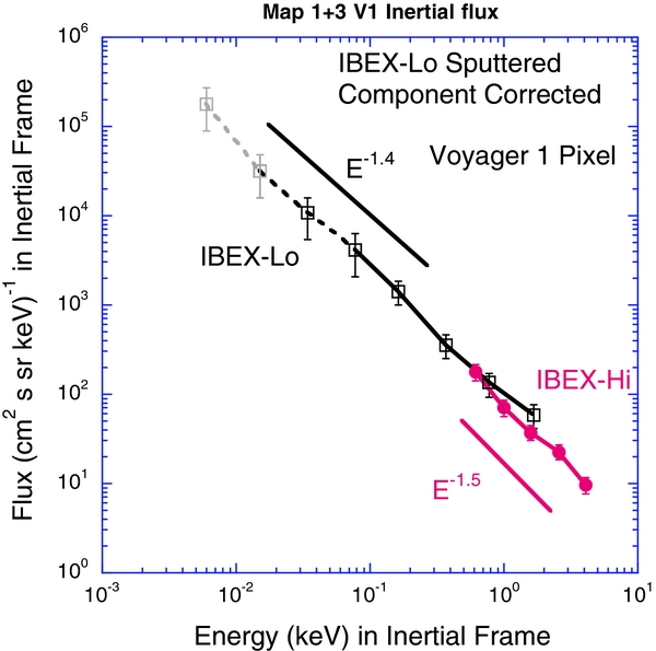
Figure 4. Composite energy spectrum from the Voyager 1 pixel. The format is the same as in Figure 3. Compared to the Ribbon pixel, this energy spectrum does not show the increased flux around 1 keV that is associated with the Ribbon and the energy spectrum is shallower at higher energies. At lower energies, the spectrum from the Voyager 1 pixel is somewhat steeper than that of the Ribbon pixel, but this may be due to contamination from ISN sputtering, especially at the lowest two energy channels of IBEX-Lo.
Download figure:
Standard image High-resolution image
Figure 5. Composite energy spectrum from the Voyager 2 pixel. The format is the same as in Figure 3. The energy spectrum from the Voyager 2 pixel is very similar to that from the Voyager 1 pixel, except that the spectrum is shallower at lower energies. This may be due to contamination from ISN sputtering in the Voyager 1 pixel at low energies.
Download figure:
Standard image High-resolution imageComparing IBEX-Hi and IBEX-Lo in Figure 3, it is evident that the two sensors measure similar fluxes in the overlapping energy range near 1 keV. The lowest energy channel of IBEX-Hi was not used because of persistent background related to the solar wind. Fluxes in this IBEX-Hi channel (now shown) are at least a factor of seven higher than those measured by IBEX-Lo at the same energy due to this background. In Figure 3, three details of the energy spectrum of heliospheric neutrals are noteworthy. First, the spectrum is very smooth below 0.4 keV, second, there is a knee in the spectrum at about 1 keV, and third, the spectral index is different at energies above 1 keV compared to energies below 0.4 keV.
The knee near 1 keV is more evident by comparing energy spectra from the Ribbon (Figure 3) and Voyager 1 (Figure 5) pixels. In the Voyager 1 pixel, the spectral index is nearly constant (at E−1.5) over the entire IBEX energy range. McComas et al. (2009c) determined a similar spectral index for the Voyager 1 pixel although they did not correct the IBEX-Lo fluxes for sputtering and they reported energies only down to 0.1 keV. At energies above 1 keV, the smaller spectral index in the Voyager 1 pixel compared to that in the Ribbon pixel is part of a general trend of decreasing spectral index with increasing ecliptic latitude (Funsten et al. 2009b). The latitude dependence on the spectral index of the energy spectrum is probably the result of a latitude dependence of the solar wind velocity (Funsten et al. 2009b). The solar wind transitions from slow (∼400 km s−1) to fast (∼700 km s−1) at mid-latitudes during solar minimum (McComas et al. 1998). Since heliospheric pick-up ions are likely the primary source of ENAs above 1 keV, the energy spectrum from a given ecliptic latitude reflects the solar wind conditions in the outer heliosphere upstream of the termination shock. If heliosheath pick-up ions at energies below the fast and slow solar wind are the primary parent source for ENAs below 0.5 keV, then they would not reflect changes from fast to slow solar wind. The similarity in the energy spectra below 0.5 keV in the Ribbon and Voyager 1 pixels is consistent with this possible source.
Comparing fluxes above and below 1 keV in Figures 3 and 4, it is apparent that while the Ribbon may extend up to the maximum energy of the IBEX-Hi sensor, it does not extend below about 0.2–0.3 keV. Fuselier et al. (2009a) reported that the Ribbon extended down to about 0.2 keV. However, this energy was in the spacecraft frame and not in the Sun's inertial frame as in Figure 3.
Above 0.15 keV, energy spectra in the Voyager 1 and Voyager 2 pixels (Figures 4 and 5) are essentially identical. The ecliptic latitudes of these two pixels are nearly equal, so spectral indices at energies above 1 keV are the same. Between 0.15 and 1 keV (that is at energies above any influence from ISN source in the Voyager 1 pixel), the spectra are also nearly identical. Below 0.1 keV, the energy spectrum in the Voyager 2 pixel has a lower spectral index than that in the Voyager 1 direction.
The Ribbon, Voyager 1, and Voyager 2 pixels are sufficiently removed from the direction of arrival of interstellar neutral hydrogen and helium so that this source may not completely dominate the energy spectra of heliospheric neutrals (at least between 0.03 and 0.1 keV). This is not the case for the Nose pixel. Therefore, Figure 6 compares IBEX-Lo and IBEX-Hi Nose pixel energy spectra from maps 1+3 and from map 2. The ISN source is evident below about 0.15 keV in the energy spectrum from maps 1+3. Because the ISN source dominates the first four energy channels of IBEX-Lo, the frame transformations to the energy and flux were not applied to these energy channels for maps 1+3. For map 2, there is no ISN source so all energy channels were frame transformed. Although fluxes from map 2 are lower than that for maps 1+3, the spectrum in the Nose pixel at energies less than 0.15 keV is not similar to that in the other 3 pixels (Figures 3–5). This result suggests that there is a background in map 2 that is not present in maps 1+3 (see the Appendix). Above about 0.3 keV, the spectra from maps 1+3 and map 2 agree reasonably well although IBEX-Hi fluxes above 0.6 keV agree much better than those from IBEX-Lo.

Figure 6. Composite energy spectra from the Nose pixel. The format is the same as in Figure 3 except that the dashed curves show fluxes measured in map 2 during the lobe intervals. At energies above 0.2 keV, the spectra from map 2 and maps 1+3 are similar to one another and these spectra are also similar to spectra from other pixels. Below 0.2 keV, the spectrum from maps 1+3 is severely contaminated by ISN sputtered background. Unfortunately, there appears to be a background that is probably associated with Earth's magnetospheric lobe that affects the energy spectrum at energies below 0.2 keV in map 2.
Download figure:
Standard image High-resolution image4. PARTIAL PRESSURES IN THE OUTER HELIOSPHERE
Extending the energy spectra below 0.5 keV offers the possibility to revisit the calculation of the partial and total pressures in the outer heliosphere. The fluxes observed by IBEX are from neutrals created in the heliosheath over a line-of-sight (LOS) distance. The parent ions exert a pressure in the heliosheath that can be estimated from the neutral flux under some important assumptions. Funsten et al. (2009b) computed the partial pressures over the energy range from 0.2 to 6 keV in the direction of the Ribbon. This calculation assumed that the ion distribution is isotropic in the Sun's reference frame. Schwadron et al. (2011) called this thermal pressure the "stationary pressure." They pointed out that the "dynamic pressure" contains a correction term because ions in the heliosheath do not have zero bulk velocity. Rather, they are moving away from the observer. With some additional assumptions, the dynamic pressure also can be calculated from the IBEX neutral fluxes.
Schwadron et al. (2011) developed a formula for the plasma pressure of an ion population that is propagating away from the observer as the integral of the plasma distribution function over velocity space. Then, they replaced the distribution function with the ion flux, using the relationship between the two and finally replaced the ion flux with the neutral flux using the relationship

Here nH is the density of neutral hydrogen in the outer heliosphere (nH = 0.1 cm−3), σ(Ep) is the energy dependent charge exchange cross-section for a proton (from Lindsay & Stebbings 2005) and LOS is the line-of-sight integration distance. The LOS is typically the thickness of the heliosheath, but because this thickness most likely differs for different directions, the LOS is carried explicitly along with the pressure in this analysis. With these substitutions, the plasma pressure multiplied by the LOS distance (expressed here in pdynes cm−2 AU so that the numbers are typically of order 10) becomes (Schwadron et al. 2011, Equation (4))
Here, m is the mass of a proton, Eo is the energy of the ion (and neutral) in the outer heliosphere, vo is the particle velocity in the rest frame of the outer heliosphere, and uR is the radial component of the bulk flow velocity of the plasma in the outer heliosphere. It is instructive to rewrite Equation (2) in terms of the stationary pressure multiplied by a correction factor and change the integral over an energy range to an evaluation of the partial pressure over an IBEX energy channel. By making these changes, the stationary pressure is directly related to the pressure calculated by Funsten et al. (2009b), the correction factor relates the stationary pressure to the dynamic pressure in Schwadron et al. (2011), and the contributions to the stationary and dynamic pressures from the lower energy channels of IBEX-Lo are described explicitly. Finally, these changes help identify where certain assumptions break down. Rewritten in this fashion, Equation (2) becomes


Here, pion is the momentum of the ion in the outer heliosheath and ΔEo is the energy passband of either IBEX-Hi or IBEX-Lo.
Several assumptions are made concerning plasma in the heliosheath and mapping of neutral atoms from their origin in the heliosheath to their observation point at 1 AU. Based on Voyager measurements extrapolated across the entire heliosheath, it is assumed that the average radial speed of the plasma in the heliosheath is ∼70 km s−1 (Schwadron et al. 2011) and that the deflection and energy change of neutrals are small as the neutral propagates from the heliosheath to 1 AU. With this last assumption, the only quantity that needs to be taken into account in the mapping of the neutral flux from 1 AU back to the heliosheath is the survival probability (Schwadron et al. 2011).
The survival probability from 100 AU to 1 AU was calculated using Schwadron et al. (2011). This calculation uses a fixed photoionization rate at 1 AU, a typical solar wind speed and density of 450 km s−1 and 6.1 cm−3, respectively, and charge exchange cross sections from Lindsay & Stebbings (2005). These assumptions introduce uncertainty in the survival probability. While these uncertainties are relatively small for higher energy neutrals (Schwadron et al. 2011), they grow significantly as the survival probability becomes less than 0.5. The uncertainty in the survival probability could be as much as a factor of 2–3 for energies less than 0.1 keV with these fixed solar wind parameters.
In Tables 2–4, a continuous spectrum from 0.03 keV to 4 keV (center energies) is created by selecting the energy channels 3–6 of IBEX-Lo and energy channels 2–6 for IBEX-Hi. Since the fluxes are the same from the two sensors in the energy overlap region near 1 keV (Figures 3–5), the IBEX-Hi fluxes (with their better statistics) are used. Each table contains the frame-transformed energy and flux at 1 AU (Columns 2 and 3). The survival probability (Column 4) is the fraction of neutrals that make it to 1 AU. These values are used to compute the frame-transformed flux at 100 AU (Column 5). The stationary pressures multiplied by LOS (Column 6, i.e., the LOS is typically taken to equal the heliosheath thickness) and correction factor (column 7) are computed from the 100 AU flux and frame-transformed energy using Equations (3) and (4). Finally, the dynamic pressure multiplied by the LOS is the stationary pressure multiplied by LOS (Column 8) multiplied by the correction factor.
The lowest two channels of IBEX-Lo are excluded from Tables 2–4. As pointed out above, that the energy and arrival angle of the neutrals is severely modified by gravitation and radiation pressure at energies below 0.02 keV. Large changes in the energy and arrival angle violate the assumptions used to compute the survival probability. In addition, survival probability of these neutrals is very low (less than 0.1), adding significant uncertainty in the pressure calculation. The next two energy channels (IBEX-Lo energy channels 3 and 4) are shown as shaded in Tables 2–4 because there is likely ISN flux present and the low survival probabilities (approximately 0.1 and 0.25) amplify this signal when computing the flux at 100 AU.
Table 2. Ribbon Pixel Flux and Pressure Summary
| Ribbon Pixel Summary | |||||||
|---|---|---|---|---|---|---|---|
| Stationary | Dynamic | ||||||
| Frame-transformed Energy | Frame-transformed Flux | Frame-transformed Flux | Pressure * LOS | Correction | Pressure * LOS | ||
| IBEX Energy Step | (keV) | (cm2 s sr kev)−1 | Survival Probability | at 100 AU | (pdynes cm−2 AU) | Factor | (pdynes cm−2 AU) |
| 3-Lo | 0.029 | 1.19E+04 | 0.09 | 1.32E+05 | 29.0 | 23.7 | 685.8 |
| 4-Lo | 0.072 | 4.17E+03 | 0.23 | 1.78E+04 | 16.9 | 9.2 | 155.9 |
| 5-Lo | 0.155 | 1.73E+03 | 0.39 | 4.43E+03 | 16.1 | 4.9 | 78.6 |
| 6-Lo | 0.358 | 4.47E+02 | 0.56 | 7.93E+02 | 11.1 | 2.9 | 32.6 |
| 2-Hi | 0.606 | 3.96E+02 | 0.65 | 6.07E+02 | 22.7 | 2.3 | 52.1 |
| 3-Hi | 0.979 | 2.05E+02 | 0.70 | 2.92E+02 | 27.0 | 1.9 | 52.1 |
| 4-Hi | 1.575 | 7.27E+01 | 0.75 | 9.75E+01 | 19.9 | 1.7 | 33.4 |
| 5-Hi | 2.522 | 3.01E+01 | 0.79 | 3.82E+01 | 17.2 | 1.5 | 25.9 |
| 6-Hi | 4.028 | 1.18E+01 | 0.82 | 1.45E+01 | 14.7 | 1.4 | 20.3 |
Download table as: ASCIITypeset image
Table 3. Voyager 1 Pixel Flux and Pressure Summary
| Voyager 1 Pixel Summary | |||||||
|---|---|---|---|---|---|---|---|
| Stationary | Dynamic | ||||||
| Frame-transformed Energy | Frame-transformed Flux | Survival | Frame-transformed Flux | Pressure * LOS | Correction | Pressure * LOS | |
| IBEX Energy Step | (keV) | (cm2 s sr kev)−1 | Probability | at 100 AU | (pdynes cm−2 AU) | Factor | (pdynes cm−2 AU) |
| 3-Lo | 0.034 | 1.07E+04 | 0.11 | 1.02E+05 | 27.3 | 20.3 | 553.6 |
| 4-Lo | 0.078 | 4.22E+03 | 0.25 | 1.71E+04 | 18.3 | 8.6 | 156.6 |
| 5-Lo | 0.163 | 1.42E+03 | 0.40 | 3.57E+03 | 14.0 | 4.7 | 65.9 |
| 6-Lo | 0.370 | 3.56E+02 | 0.57 | 6.29E+02 | 9.3 | 2.9 | 26.7 |
| 2-Hi | 0.621 | 1.78E+02 | 0.66 | 2.71E+02 | 10.5 | 2.3 | 24.0 |
| 3-Hi | 0.998 | 7.11E+01 | 0.70 | 1.01E+02 | 9.6 | 1.9 | 18.5 |
| 4-Hi | 1.598 | 3.75E+01 | 0.75 | 5.03E+01 | 10.5 | 1.7 | 17.5 |
| 5-Hi | 2.551 | 2.28E+01 | 0.79 | 2.89E+01 | 13.2 | 1.5 | 19.9 |
| 6-Hi | 4.065 | 9.66E+00 | 0.82 | 1.18E+01 | 12.1 | 1.4 | 16.7 |
Download table as: ASCIITypeset image
Table 4. Voyager 2 Pixel Flux and Pressure Summary
| Voyager 2 Pixel Summary | |||||||
|---|---|---|---|---|---|---|---|
| Stationary | Dynamic | ||||||
| Frame-transformed Energy | Frame-transformed Flux | Survival | Frame-transformed Flux | Pressure * LOS | Correction | Pressure * LOS | |
| IBEX Energy Step | (keV) | (cm2 s sr kev)−1 | Probability | at 100 AU | (pdynes cm−2 AU) | Factor | (pdynes cm−2 AU) |
| 3-Lo | 0.032 | 6.83E+03 | 0.10 | 6.92E+04 | 17.0 | 21.6 | 368.1 |
| 4-Lo | 0.075 | 3.52E+03 | 0.24 | 1.46E+04 | 14.8 | 8.8 | 131.0 |
| 5-Lo | 0.159 | 1.66E+03 | 0.40 | 4.20E+03 | 15.9 | 4.8 | 76.2 |
| 6-Lo | 0.365 | 2.97E+02 | 0.57 | 5.26E+02 | 7.6 | 2.9 | 22.0 |
| 2-Hi | 0.615 | 1.63E+02 | 0.65 | 2.50E+02 | 9.5 | 2.3 | 21.8 |
| 3-Hi | 0.990 | 7.45E+01 | 0.70 | 1.06E+02 | 10.0 | 1.9 | 19.2 |
| 4-Hi | 1.588 | 4.85E+01 | 0.75 | 6.49E+01 | 13.4 | 1.7 | 22.5 |
| 5-Hi | 2.538 | 2.28E+01 | 0.79 | 2.90E+01 | 13.2 | 1.5 | 19.8 |
| 6-Hi | 4.049 | 9.13E+00 | 0.82 | 1.12E+01 | 11.4 | 1.4 | 15.7 |
Download table as: ASCIITypeset image
The stationary pressures in Tables 2–4 are roughly equal at each energy level, except in the energy range from 0.35 to 2.5 keV in the Ribbon pixel (Table 2), where the Ribbon exerts about a factor of two more pressure than in the Voyager 1 and 2 pixels. Otherwise, contributions to the stationary pressure at lower energies are the same as those at higher energies. This nearly energy-independent contribution is simply a reflection of the ∼E−1.5 slope of the energy spectrum over the IBEX energy range.
Unlike the stationary pressure, the dynamic pressure computed under the assumptions that went into Equations (3) and (4) is significantly more at lower energies than at higher energies. The difference between stationary and dynamic pressures is the correction factor, which is approximately a constant/v2o when the neutral velocity is less than the radial velocity in the heliosheath (Eo ∝ v2o < u2r). When the bulk of the plasma is moving radially away from the observer at a speed of ur, the plasma pressure must become very high to account for the observed neutral fluxes at 1 AU. One solution to this pressure imbalance is to assume that there are turbulent fluctuations in the heliosheath that result in a significant fraction of low energy ions with velocity vectors directed back into the heliosphere (Gloeckler & Fisk 2010). In Table 2, the correction factor becomes large at energies of the order of 0.07 keV, or velocities of the order of 100 km s−1. If these fluctuations exist in the heliosheath, then they should be of the same order of magnitude. Thus, at energies higher than 0.07 keV, the plasma distribution in the heliosheath is described as a population of ions with an average bulk radial velocity of 70 km s−1. However, at lower energies, turbulent fluctuations violate this assumption that goes into the derivation of Equations (3) and (4). Some caution should be taken with this interpretation because the fluxes in the energy channels 3 and 4 of IBEX-Lo likely contain an ISN signal. The pixel that most likely contains the lowest ISN signal is the Voyager 2 pixel (Table 4), which still shows a significant divergence in the dynamic pressure in energy channels 3 and 4 of IBEX-Lo.
Combining the neutral flux at 100 AU in the Voyager 1 pixel (Table 3) with higher energy fluxes from the Cassini INCA (Krimigis et al. 2009) and SoHO HSTOF (Hilchenbach et al. 1998; Kallenbach et al. 2005) in the same direction, Figure 7 shows the ENA spectrum at 100 AU from 0.03 to 100 keV (the lowest two energy channels of IBEX-Lo are not used here). The light-blue curve in Figure 7 shows the fit to the original IBEX data above 0.15 keV, the INCA data and the HSTOF data (Gloeckler & Fisk 2010). The difference between the original fit to the IBEX data above 0.15 keV and the current data shown in Figure 7 may be due to a slightly different survivability estimate for these data.

Figure 7. Composite ENA spectrum from IBEX, Cassini INCA, and SoHO HSTOF from the Voyager 1 pixel. All fluxes have been mapped to 100 AU by accounting for the survival probability and all fluxes have been transformed to an inertial frame. The light blue curve that extends over the entire range of the ENA measurements represents a fit (Gloeckler & Fisk 2010) to fluxes greater than 0.16 keV that were published prior to 2010. This fit is based on four proton populations in the heliosheath: (a) heliosheath solar wind, (b) heliosheath pick-up ions, (c) heliosphere pick-up ions, and (d) heliosheath suprathermal tails. Through charge exchange with the ambient neutral gas each of these four populations is converted to ENAs with each of the four ENA heliosheath populations predominating at progressively higher energies as shown in the figure. The IBEX fluxes shown here extend below 0.16 keV and are higher that the previously reported fluxes by a factor of ∼2.5 and ∼2 at 0.16 and 0.37 keV, respectively. See Gloeckler & Fisk (2010) for a more detailed discussion of how each of the four ENA populations was obtained.
Download figure:
Standard image High-resolution imageGloeckler & Fisk (2010) identify four proton populations in the heliosheath that by charge exchange (using the best charge-exchange cross-sections) with the ambient neutral gas (using the best available heliosheath neutral hydrogen densities) become corresponding ENA populations: (a) heliosheath solar wind, (b) heliosheath pick-up ions, (c) heliosphere pick-up ions, and (d) heliosheath suprathermal tails. The light blue curve represents the ENA spectrum, obtained by combining the four ENA populations, that spans the entire energy range in Figure 7. In the Gloeckler & Fisk empirical fit, compressional strong turbulence in the heliosheath beyond ∼110 AU, with sunward-directed speeds of ∼150 km s−1, is needed to account for the ENA fluxes below about 1 keV. Without this turbulence, ENA populations (a) and most of (b) would have no sunward moving components, and would thus never reach 1 AU. The amplitude of the turbulent speed (not yet measured by Voyager 2) also needs to be larger to better match the IBEX fluxes between 0.2 and 0.7 keV in Figure 7.
Other models (e.g., Prested et al. 2008) predict higher fluxes for population (c) at 1 keV and therefore may account for the IBEX fluxes near this energy without invoking strong turbulence (Schwadron et al. 2009). However, in the energy range between 0.2 and 0.7 keV, it is difficult to explain the high ENA fluxes without including a parent population of low energy ions beyond the termination shock. Populations (a) and (b) in Figure 7 combined with strong turbulence in the outer heliosheath constitute one explanation for the ENA fluxes in this energy range, but other explanations may be found in the future.
The very high fluxes in Figure 7 below 0.2 keV are difficult to explain by any of the current models. However, as pointed out above, the ISN signal may contribute substantially to the total flux in the Voyager 1 direction.
5. CONCLUSIONS
Using combined sky maps, neutral fluxes over the entire IBEX energy range in the Ribbon (at southern latitudes near the equator), Voyager 1, Voyager 2, and Nose pixels were presented in Figures 3–6. The Ribbon is a phenomenon that occurs over a finite range of energies from about ∼0.2–0.3 keV to ∼2–4 keV. At energies less than 0.2 keV, the heliospheric neutral flux is similar in the Ribbon, Voyager 1, and Voyager 2 pixels. Differences may be due to contamination of the heliospheric neutral flux by sputtering within the IBEX-Lo sensor by interstellar neutrals. Fluxes measured during intervals when the spacecraft was in Earth's magnetospheric lobes (a region where energetic ion fluxes are very low) were used in an attempt to quantify the ISN signal in combined maps 1+3. Unfortunately, there appears to be a background at low energies in Earth's lobes and fluxes at low energies, when frames transformed to an inertial frame are higher in the lobes than in the solar wind (see the Appendix). Thus, it is difficult to separate possible differences in, for example, the low-energy heliospheric fluxes in the Voyager 1 and 2 pixels (perhaps due to longer LOS integration lengths) from contamination by effects generated by ISN neutrals within the sensor. Indeed, the energy spectra from the Ribbon, Voyager 1 and Voyager 2 pixels are nearly identical from 0.1 to 0.2 keV (where the ISN signal does not contribute). Sputtering by ISN species produces an apparent power-law spectrum in energy for the lowest four energy channels. The progressive decrease in the spectral index below 0.5 keV in the Voyager 1 to the Ribbon to the Voyager 2 pixels is consistent with a decreasing contamination from the ISN signal, with the Voyager 2 pixel probably the least contaminated (but certainly not free of contamination) from this background. The ISN signal renders the low energy (below 0.2 keV) fluxes in the Nose direction essentially useless for investigating heliospheric neutral fluxes in that direction. Relative levels of confidence in the measurements are illustrated in Figures 3–7 and Figure 11 by the connecting lines and shading of the data points. Solid lines connect data points where there is confidence that the points are relatively free of contamination from background and ISN sources, dashed lines indicate points where there is likely contamination from ISN, and other sources and gray points (measurements at the lowest two energies) indicate data with the least confidence.
The heliospheric neutral fluxes were used to estimate ion partial pressures multiplied by LOS distance in the heliosheath. Low energy ions contribute approximately equally to the stationary pressure when compared to higher energy ions. The same would be true for the dynamic pressure if turbulence were assumed to exist with fluctuation levels of the order of 50–100 km s−1. Thus, the low-energy neutral flux reveals characteristics of the plasma in the heliosheath that are important for determining neutral fluxes observed at 1 AU.
Combining IBEX observations discussed here with observations at higher energies from Cassini INCA and SoHO HSTOF, the ENA spectrum from 0.03 to 100 keV is shown in Figure 7 for the Voyager 1 pixel. The combined IBEX-Cassini SoHO ENA spectrum, that was available in 2010 in the energy range from 0.16 keV to ∼80 keV, was fit with a model using various ion populations in the heliosheath that by charge exchange with the ambient neutral gas created ENAs over this energy range (Gloeckler & Fisk 2010). The current IBEX spectrum at energies below ∼0.5 keV cannot be explained easily based solely on ENA populations (a) and (b), and may require a new low-energy ENA parent ion population from beyond the termination shock. A similar result is obtained in the Voyager 2 pixel over the energy range from 0.03 to 0.2 keV since fluxes are the same as in the Voyager 1 pixel within the measurement uncertainties.
These results open the possibility for further study and modeling of low energy fluxes in other parts of the sky maps not affected by ISN signal (e.g., the ecliptic poles and tail direction). Further study of these regions, combined with simulations of the conditions in the heliosheath, should improve the understanding of the origin of the heliospheric neutrals observed at 1 AU and the conditions in the heliosheath that determine their flux levels.
Support for this study comes from NASA's Explorer program. IBEX is the result of efforts from a large number of scientists, engineers, and others. All who contributed to this mission share in its success.
APPENDIX
In principle, the ISN signal can be removed from odd numbered maps by using observations from map 2 (during the interval from approximately 2009 June to December). During part of the accumulation of the second map (in orbits 41–46, from 2009 August 10 to September 25), the IBEX spacecraft was primarily in Earth's magnetotail, most of the time in the plasma sheet. This region of hot (several kev, extending to tens of kev), relatively slow (<100 km s−1), and relatively dense (∼1 cm−3) plasma produces a significant background in IBEX-Lo as well as significant energetic ion flux in the background monitor. However, during parts of orbits 41–46, the spacecraft was in Earth's (southern) lobe. These lobe intervals are characterized by very low ion fluxes in the background monitor because there is very little plasma in this magnetospheric region and most of the plasma is at energies much less than the approximately 15 keV low-energy cutoff of the background monitor. Figure 8 shows an example of a lobe interval during IBEX orbit 46 (from 2009 September 18 to 25). The top panel shows the IBEX orbit projected into the ecliptic plane as viewed from the north ecliptic pole. Most of the orbit is inside the nominal location of Earth's magnetopause, but apogee is in the magnetosheath between the bow shock and magnetopause. The bottom panel shows a spin angle (NEP angle)—time spectrogram of background monitor counts s−1 for the entire orbit. For most of the orbit, the spacecraft is in the magnetosheath or plasma sheet and background monitor countrates are relatively high (>100 counts/96 second accumulation interval). However, centered on day 268 (2009 September 25), the spacecraft is in the lobe and background monitor countrates are very low (<10 counts/accumulation period). During orbits 41–46, there are several intervals when the spacecraft was in the lobe. For these orbits, IBEX viewed ecliptic longitudes −90º to −120º and 60º to 90º. This view includes the Voyager 1, Nose, and Ribbon pixels show in Figure 1. The ISN helium flux does not interfere with IBEX observations in this part of map 2 because the ISN helium direction is the opposite direction from the Nose and the ISN helium energy is only 8 eV.

Figure 8. Composite of an ecliptic plane projection of IBEX orbit 46 and a spin-time spectrogram of the background monitor count rate (for ions >15 keV) over the orbit. During the orbit, the spacecraft is in Earth's magnetosphere or in the magnetosheath and background monitor count rates are relatively high (>100 counts/sample period). However, during some intervals, the spacecraft is in Earth's magnetospheric lobe and energetic ion fluxes are very low. These periods from the sky map 2 interval were selected to create a map that was not contaminated by energetic ion or ISN sputtering backgrounds.
Download figure:
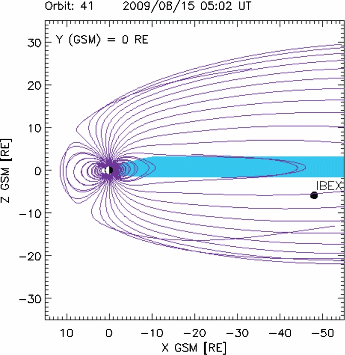
Standard image High-resolution imageFigure 9 shows the IBEX spacecraft location in Earth's southern lobe region during a portion of orbit 41 (centered on 2009 August 15 at 0502 UT). The Sun is to the left and the magnetic field lines from the Tsyganenko (1995) magnetic field model are shown. The blue region is Earth's plasma sheet, where there are very high fluxes of energetic ions. (Neutrals from the plasma sheet were successfully imaged recently for the first time by IBEX (McComas et al. 2011b)). The IBEX sensors view in a plane perpendicular to the Earth–Sun line. At spin angles of 0°, the sensors view in the direction of the plasma sheet and at spin angles of 180°, the sensors view in the direction of the southern ecliptic pole opposite the plasma sheet direction.

Figure 9. Noon–midnight meridonal cut through a model of Earth's magnetosphere. The Sun is to the left and magnetic field lines in Earth's lobe regions extend off to the right above and below the nominal location of Earth's plasma sheet (blue region). In the plasma sheet, energetic ion fluxes are very high, while in the lobe they are very low. The IBEX spacecraft position is shown for orbit 41 on 2009 August 15 at 05 UT.
Download figure:
Standard image High-resolution imageFigure 10 shows a stacked plot of countrates (in arbitrary units) from four energy channels of IBEX-Lo and one energy channel of IBEX-Hi as a function of spin angle from the map 2 observations in Earth's lobe. Both IBEX-Lo energy channel 7 and IBEX-Hi energy channel 3 measure neutrals at approximately 1 keV, so the count rate profiles should be very similar. Indeed, the red and black (with open squares) curves trace the same fluxes and the Ribbon is evident in the 240° direction. Furthermore, there is evidence of a Compton–Getting (CG) effect in the count rate versus spin curves for these two energies. They show a general trend of increasing countrate up to 90° and then a decrease to 180° because neutrals are rammed into the sensors at 90° and therefore have higher fluxes due to the CG effect. The opposite trend should be seen from 180° to 360°; however, the high fluxes in the Ribbon mask the CG effect on the underlying globally distributed flux.

Figure 10. Stack plot of spin-angle–count-rate curves for four IBEX energy channels. These curves are taken from map 2 during intervals when the spacecraft was in the lobe. The red (solid circles) and black (open squares) curves show the countrate from an IBEX-Lo and an IBEX-Hi energy channel that measure nearly the same energy. The Ribbon is seen at 240º in both energy channels. At 0.11 keV (blue curve with solid squares), the Ribbon is still evident. At 0.055 keV (black curve with solid diamonds), it is not clear if the Ribbon is still present or if there is simply a broad peak centered at approximately 120º. The IBEX-Lo sensor views perpendicular to the Earth–Sun line and, at 120º, it was viewing away from the nominal plasma sheet direction. Therefore, the background fluxes at low energies are likely associated with low energy ions or neutrals in the lobe.
Download figure:
Standard image High-resolution imageThe blue curve shows the count rate from IBEX-Lo energy channel 4 (at 0.11 keV center energy). The Ribbon is still evident near 240°, but there is less evidence of a CG effect from 0° to 180°. Less evidence of the CG effect at 0.11 keV when compared to 1 keV is contrary to the expectation that the CG effect should increase with decreasing energy (provided that the slope of the energy spectrum is relatively constant over this energy range). Less evidence of a CG effect suggests that there is a background at lower energies that is of the same order as the heliospheric neutral signal. The continued presence of the Ribbon suggests that this background may be as intense as the globally distributed heliospheric flux, but not as high as the Ribbon flux. The black curve (with solid diamonds) shows the count rate from IBEX-Lo energy channel 2. While there is a peak at 240°, it is not clear if this is the Ribbon or simply part of a much wider centered approximately at 180°. There is no longer any consistency with the CG effect despite the fact that these measurements are made at a very low energy, suggesting that this background, associated with Earth's magnetosphere, dominates the heliospheric flux.
Figure 11 shows a comparison of frame-transformed fluxes for the Voyager 1 pixel from maps 1+3 and map 2. If fluxes in both of these maps were free of background, then the two curves should be identical. At high energies, above 1 keV, the two curves are essentially identical. However, below about 0.5 keV, the two curves begin to deviate from one another until, at the lowest energies, the fluxes in map 2 are more than 10 times those in maps 1+3. Higher fluxes in map 2 are consistent with the presence of a background encountered in Earth's magnetospheric lobes at energies below 0.5 keV that is not present in the solar wind. This background does not appear to be coming from the plasma sheet. Instead, it may be associated with low-energy ion beams in Earth's lobes. Unfortunately, this comparison of map 2 with maps 1+3 does not indicate that the fluxes in maps 1+3 are free of background. It only indicates that the even number maps, when the IBEX spacecraft is in Earth's magnetosphere, cannot be used at this time to confirm heliospheric flux levels below about 0.5 keV.

Figure 11. Comparison of energy spectra from the Voyager 1 pixel for maps 1+3 (black and gray for IBEX-Lo and red for IBEX-Hi) and map 2 (green for IBEX-Lo and blue for IBEX-Hi). The two curves agree at high energies but diverge below 0.7 keV. This deviation is evidence of a low-energy background in the lobe (from map 2) that is not present in the solar wind (from maps 1+3).
Download figure:
Standard image High-resolution image