


ABSTRACT
Surveys above 10 keV represent one of the best resources to provide an unbiased census of the population of active galactic nuclei (AGNs). We present the results of 60 months of observation of the hard X-ray sky with Swift/Burst Alert Telescope (BAT). In this time frame, BAT-detected (in the 15–55 keV band) 720 sources in an all-sky survey of which 428 are associated with AGNs, most of which are nearby. Our sample has negligible incompleteness and statistics a factor of ∼2 larger over similarly complete sets of AGNs. Our sample contains (at least) 15 bona fide Compton-thick AGNs and 3 likely candidates. Compton-thick AGNs represent ∼5% of AGN samples detected above 15 keV. We use the BAT data set to refine the determination of the log N–log S of AGNs which is extremely important, now that NuSTAR prepares for launch, toward assessing the AGN contribution to the cosmic X-ray background. We show that the log N–log S of AGNs selected above 10 keV is now established to ∼10% precision. We derive the luminosity function of Compton-thick AGNs and measure a space density of 7.9+4.1− 2.9 × 10⁻⁵ Mpc−3 for objects with a de-absorbed luminosity larger than 2 × 1042 erg s−1. As the BAT AGNs are all mostly local, they allow us to investigate the spatial distribution of AGNs in the nearby universe regardless of absorption. We find concentrations of AGNs that coincide spatially with the largest congregations of matter in the local (⩽85 Mpc) universe. There is some evidence that the fraction of Seyfert 2 objects is larger than average in the direction of these dense regions.
Export citation and abstract BibTeX RIS
1. INTRODUCTION
There is a general consensus that the cosmic X-ray background (CXB), discovered more than 40 years ago (Giacconi et al. 1962), is produced by integrated emission of active galactic nuclei (AGNs). Indeed, below ∼3 keV sensitive observations with Chandra and XMM-Newton have directly resolved as much as 80% of the CXB into AGNs (Worsley et al. 2005; Luo et al. 2011). However, above 5 keV, due to the lack of sensitive observations, most of the CXB emission is at present unresolved. Population synthesis models have successfully shown, in the context of the AGN unified theory (Antonucci 1993), that AGNs with various level of obscuration and at different redshifts can account for 80%–100% of the CXB up to ∼100 keV (Comastri et al. 1995; Gilli et al. 2001; Treister & Urry 2005). In order to reproduce the spectral shape and the intensity of the CXB, these models require that Compton-thick AGNs (NH ⩾ 1.4 × 1024 cm−2) contribute ∼10% of the total CXB intensity. With such heavy absorption, Compton-thick AGNs have necessarily to be numerous, comprising perhaps up to 30%–50% of the AGN population in the local universe (e.g., Risaliti et al. 1999). However, it is still surprising that only a very small fraction of the population of Compton-thick AGNs have been uncovered so far (Comastri 2004; Della Ceca et al. 2008b, and references therein).
Studies of AGNs are best done above 10 keV where the nuclear radiation pierces through the torus for all but the largest column densities. Focusing optics like those mounted on NuSTAR and ASTRO-H (respectively, Harrison et al. 2010; Takahashi et al. 2010) will allow us to reach, for the first time, sensitivities ⩽10−13 erg cm−2 s−1 above 10 keV, permitting us to resolve a substantial fraction of the CXB emission in this band. Given their small field of views (FOVs), those instruments will need large exposures in order to gather reasonably large AGN samples. Because of their good sensitivity, the AGN detected by NuSTAR and ASTRO-H should be at redshift ∼1, but, due to the small area surveyed, very few if any will be at much lower redshift.
All-sky surveys, like those performed by Swift/Burst Alert Telescope (BAT) and INTEGRAL above 10 keV, are very effective in making a census of nearby AGNs, thus providing a natural extension to more sensitive (but with a narrower FOV) missions. Here, we report on the all-sky sample of AGNs detected by BAT in 60 months of exposure. Our sample comprises 428 AGNs detected in the whole sky and represents a factor of ∼2 improvement in number statistics when compared to previous complete samples (e.g., Burlon et al. 2011). In this paper, we present the sample and refine the determination of the source count distribution and of the luminosity function (LF) of AGNs. This is especially important considering the upcoming launch of NuSTAR (scheduled for 2012 March) as it allows us to make accurate predictions for the expected space densities of distant AGNs. We also use the BAT sample to investigate the spatial distribution of AGNs in the local universe. We leave for an upcoming publication the follow-up of all new sources using 2–10 keV data and the determination of the absorption distribution.
This paper is organized as follows: the BAT observations are discussed in Section 2, while Sections 3.1 and 3.2 discuss, respectively, the source count distribution and the LF of AGNs. In Section 4, we present a measurement of the overdensity of AGNs in the local universe, while in Section 5 the prospects for the detection of AGNs by NuSTAR are discussed in the framework of the BAT observations and population synthesis models. Finally, Section 6 summarizes our findings. Throughout this paper, we assume a standard concordance cosmology (H0 = 71 km s−1 Mpc−1, ΩM = 1 − ΩΛ = 0.27).
2. PROPERTIES OF THE SAMPLE
The BAT (Barthelmy et al. 2005) onboard the Swift satellite (Gehrels et al. 2004) represents a major improvement in sensitivity for imaging of the hard X-ray sky. BAT is a coded mask telescope with a wide FOV (120° × 90° partially coded) aperture sensitive in the 15–200 keV range. Thanks to its wide FOV and its pointing strategy, BAT monitors continuously up to 80% of the sky every day achieving, after several years, deep exposures across the entire sky. Results of the BAT survey (Markwardt et al. 2005; Ajello et al. 2008a; Tueller et al. 2008) show that BAT reaches a sensitivity of ∼1 mCrab5 in 1 Ms of exposure. Given its sensitivity and the large exposure already accumulated in the whole sky, BAT is an excellent instrument for studying populations whose emission is faint in hard X-rays.
For the analysis presented here, we use 60 months of Swift/BAT observations taken between 2005 March and 2010 March. Data screening and processing was performed according to the recipes presented in Ajello et al. (2008a) and Ajello et al. (2008b). The chosen energy interval is 15–55 keV. The all-sky image is obtained as the weighted average of all the shorter observations. The final image shows a Gaussian normal noise and we identified source candidates as those excesses with a signal-to-noise ratio (S/N) ⩾ 5σ. The final sample comprises 720 sources detected all-sky. Identification of these objects was performed by cross-correlating our catalog with the catalogs of Tueller et al. (2008), Cusumano et al. (2010), Voss & Ajello (2010), and Burlon et al. (2011). Whenever available we used the newest optical identifications provided by Masetti et al. (2008, 2009, 2010). Of the 720 all-sky sources, only 37 (i.e., ∼5%) do not have a firm identification. This small incompleteness does not change when excluding or including the Galactic plane. Of the 720 objects, 428 are identified with AGNs. This represents an improvement of a factor >2 in the number of detected AGNs with respect to previous complete samples (e.g., Ajello et al. 2009a; Burlon et al. 2011). Cusumano et al. (2010) recently reported on the sample of sources detected by BAT in 58 months of observations. Their catalog is constructed using three energy bands and selecting ⩾4.8σ excesses in any of the three bands. As such, their catalog is larger than the one presented here. However, for the scope of this and future analyses (e.g., a follow-up work of that presented in Burlon et al. 2011) it is important to have a clean sample whose selection effects are well understood and can be accounted for during the analysis.
Figure 1 shows the sky coverage of the BAT survey. It is apparent that the limiting flux is ∼0.45 mCrab (∼5.5 × 10⁻¹² erg cm−2 s−1) and that the BAT survey becomes complete (for the whole sky) for source fluxes ⩾1 mCrab. The sensitivity scales nicely with the inverse of the square root of the exposure time as testified by the limiting sensitivity of 0.6 mCrab reached in 36 months of observations (Ajello et al. 2009b).
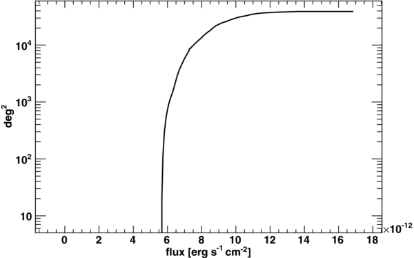
Figure 1. Sky coverage of the BAT survey for the 15–55 keV band and for sources detected all-sky above the 5σ level.
Download figure:
Standard image High-resolution image2.1. Jet-dominated and Disk-dominated Objects
Jet-dominated AGNs (radio galaxies and blazars) constitute a ∼15% fraction of the BAT samples (see, e.g., Ajello et al. 2009a). This is confirmed also here where 67 AGNs (out of the 428 AGNs) are classified as either radio galaxies or blazars. The remaining 361 AGNs are associated with objects optically classified as Seyfert galaxies (323 objects) or with nearby galaxies (38 sources), through the detection of a soft X-ray counterpart, for which an optical classification is not yet available. The full sample is reported in Table 1. For all the sources, k-corrected LX luminosities were computed according to
where FX is the X-ray energy flux in the 15–55 keV band and ΓX is the photon index. This assumes that the source spectra are adequately well described by a power law in the 15–55 keV band in agreement with what was found by Ajello et al. (2008b), Tueller et al. (2008), and Burlon et al. (2011). Unless noted otherwise (i.e., Section 3.3), luminosities are not corrected for absorption along the line of sight since this correction is different than unity (in the 15–55 keV band) only for Compton-thick AGNs (see Figure 11 in Burlon et al. 2011) and does not introduce any apparent bias in any of the results shown in the next sections.
Table 1. The 428 AGNs Detected by BAT
| Swift Name | R.A. | Decl. | Position Error | Flux | S/N | ID | Typea | Redshift | Photon Index | log LX |
|---|---|---|---|---|---|---|---|---|---|---|
| (J2000) | (J2000) | (arcmin) | (10−11 cgs) | |||||||
| J0004.2+7018 | 1.050 | 70.300 | 6.551 | 0.76 | 5.5 | 2MASX J00040192+7019185 | AGN | 0.0960 | 2.04 ± 0.46 | 44.2 |
| J0006.2+2010 | 1.571 | 20.168 | 3.276 | 1.06 | 6.5 | Mrk 335 | Sy1 | 0.0254 | 2.60 ± 0.32 | 43.2 |
| J0010.4+1056 | 2.622 | 10.947 | 2.281 | 1.85 | 11.0 | QSO B0007+107 | BLAZAR | 0.0893 | 2.23 ± 0.20 | 44.6 |
| J0018.9+8135 | 4.732 | 81.592 | 4.720 | 0.94 | 6.5 | QSO J0017+8135 | BLAZAR | 3.3600 | 2.51 ± 0.52 | 48.3 |
| J0021.2−1908 | 5.300 | −19.150 | 4.773 | 0.92 | 5.1 | 1RXSJ002108.1-190950 | AGN | 0.0950 | 1.96 ± 0.45 | 44.3 |
| J0025.0+6826 | 6.264 | 68.436 | 4.721 | 0.78 | 5.6 | IGR J00256+6821 | Sy2 | 0.0120 | 1.66 ± 0.33 | 42.4 |
| J0033.4+6125 | 8.351 | 61.431 | 4.274 | 1.01 | 7.3 | IGR J00335+6126 | AGN | 0.1050 | 2.46 ± 0.28 | 44.5 |
| J0034.6−0423 | 8.651 | −4.400 | 6.165 | 0.92 | 5.2 | 2MASX J00343284-0424117 | AGN | 0.0000 | 1.79 ± 0.43 | ⋅⋅⋅ |
| J0035.8+5951 | 8.965 | 59.852 | 2.095 | 2.05 | 14.8 | 1ES 0033+59.5 | BLAZAR | 0.0860 | 2.74 ± 0.18 | 44.6 |
| J0038.5+2336 | 9.648 | 23.600 | 5.132 | 1.01 | 6.2 | Mrk 344 | AGN | 0.0240 | 1.80 ± 0.59 | 43.1 |
| J0042.8−2332 | 10.701 | −23.548 | 3.068 | 2.52 | 14.7 | NGC 235A | Sy2 | 0.0222 | 1.90 ± 0.11 | 43.4 |
Notes. aAGNs are sources lacking an exact optical classification.
Only a portion of this table is shown here to demonstrate its form and content. A machine-readable version of the full table is available.
Download table as: DataTypeset image
Figure 2 shows the position of the 428 sources in the luminosity–redshift plane for the different optical classifications reported in Table 1. The BAT AGN sample spans almost eight decades in luminosity and includes sources detected from z ≈ 0.001 (i.e., ∼4 Mpc) up to z ≈ 4. It is also evident that Seyfert galaxies dominate the low-luminosity part of the sample, while blazars and radio galaxies dominate the high-luminosity part of the sample. The increased exposure of BAT allows us to detect fainter AGNs with respect to previous samples. Indeed, the average flux of the Seyfert-like AGN decreased by ∼20% when comparing it to the sample of AGNs reported in Burlon et al. (2011). Since the average redshift in the two samples is very similar, this translates into a larger number of low-luminosity AGNs.
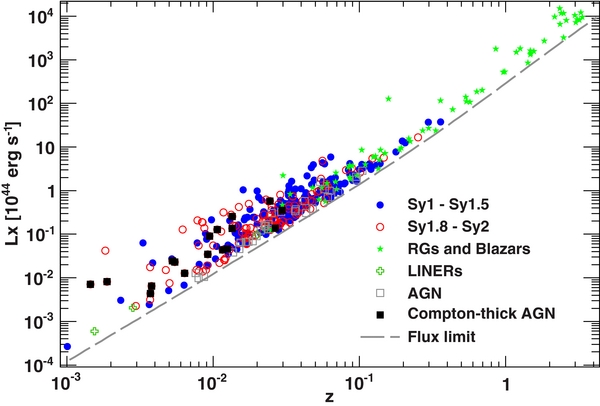
Figure 2. Position on the luminosity–redshift plane of the 428 AGNs detected by BAT in the 15–55 keV band. The color coding reflects the optical classification reported in Table 1. AGNs are sources lacking an exact optical classification. The black squares mark the position of the Compton-thick AGN reported in Table 2. Note that their luminosities were not corrected for absorption (see the text for details). The dashed line shows the flux limit of the BAT survey of 5.5 × 10⁻¹² erg cm−2 s−1.
Download figure:
Standard image High-resolution image2.2. Compton-thick AGNs
Hard X-ray-selected samples are among the best resources to uncover Compton-thick AGNs which are otherwise difficult to detect. A detailed measurement of the absorbing column density of all the AGNs in this sample is beyond the scope of this paper and left for a future publication. However, in order to determine the likely candidates, it is possible to cross-correlate our source list with catalogs of Compton-thick AGNs. Our AGN catalog contains all nine Compton-thick AGNs reported by Burlon et al. (2011) and the six additional Compton-thick AGNs reported in the list of bona fide objects of Della Ceca et al. (2008b). There are three additional sources which are labeled as Compton-thick candidates by (Della Ceca et al. 2008b, see their Table 2) which are also detected in this sample. The full list of 18 known Compton-thick AGNs contained in this sample is reported in Table 2. It is clear that the number of (likely) Compton-thick AGNs is doubled with respect to the sample of Burlon et al. (2011) and that Compton-thick AGNs represent a "steady" 5% fraction (i.e., ∼18/361) of AGN samples selected above 10 keV.
Table 2. Known Compton-thick AGNs Detected in the BAT Sample
| Name | Type | Redshift | R.A. | Decl. | NH |
|---|---|---|---|---|---|
| (J2000) | (J2000) | (1024 cm−2) | |||
| NGC 424 | Sy2 | 0.011588 | 17.8799 | −38.0944 | 1.99 |
| NGC 1068 | Sy2 | 0.003787 | 40.7580 | −0.0095 | >10 |
| NGC 1365a,b | Sy1.8 | 0.005460 | 53.4442 | −36.1292 | 3.98 |
| CGCG 420-015 | Sy2 | 0.029621 | 73.3804 | 4.0600 | 1.46 |
| SWIFT J0601.9-8636 | Sy2 | 0.006384 | 91.1972 | −86.6245 | 1.01 |
| Mrk 3 | Sy2 | 0.013509 | 93.9722 | 71.0311 | 1.27e |
| UGC 4203a,c | Sy2 | 0.013501 | 121.0585 | 5.1217 | >1.00e |
| NGC 3079 | Sy2 | 0.003720 | 150.4701 | 55.6978 | 5.40 |
| NGC 3281 | Sy2 | 0.010674 | 157.9743 | −34.8571 | 1.96e |
| NGC 3393 | Sy2 | 0.012500 | 162.1000 | −25.1539 | 4.50 |
| NGC 4939 | Sy1 | 0.010374 | 196.1000 | −10.3000 | >10e |
| NGC 4945 | Sy2 | 0.001878 | 196.3726 | −49.4742 | 2.20e |
| Circinus Galaxy | Sy2 | 0.001447 | 213.3828 | −65.3389 | 4.30e |
| NGC 5728 | Sy2 | 0.009467 | 220.6916 | −17.2326 | 1.0 |
| ESO 138-1 | Sy2 | 0.009182 | 253.0085 | −59.2386 | 1.5e,f |
| NGC 6240 | Sy2 | 0.024480 | 253.3481 | 2.3999 | 1.83 |
| NGC 6552a,d | Sy2 | 0.026550 | 270.0981 | 66.6000 | >1.00e |
| NGC 7582 | Sy2 | 0.005253 | 349.6106 | −42.3512 | 1.10 |
Notes. Unless written explicitly, the values of the absorbing column density come from Burlon et al. (2011). aPart of the sample of candidate Compton-thick objects in Della Ceca et al. (2008b). bNGC 1365 is a complex source that shows a column density that can vary from log NH ≈ 23 to ⩾ 24 on timescales of ∼10 hr (Risaliti et al. 2009b). According to Risaliti et al. (2009a), the source has an absorber with log NH ≈ 24.6 which covers ∼80% of the source. cUGC 4203 (also called the "Phoenix" galaxy) is known to exhibit changes in the absorbing column density from the Compton-thin to the Compton-thick regime (see, e.g., Risaliti et al. 2010). dReported to be Compton-thick by Reynolds et al. (1994), and Bassani et al. (1999). eFor the value of the absorbing column density, see Della Ceca et al. (2008b) and references therein. fPiconcelli et al. (2011) report that this source might be absorbed by log NH ⩾ 25.
Download table as: ASCIITypeset image
The redshift distribution of Compton-thick AGNs is also different than that of the whole AGN sample. The median redshift of the Compton-thick AGN of Table 2 is 0.010 while that of the entire AGN sample is 0.029. Compton-thick AGNs can be detected by BAT only within a distance of ∼100 Mpc beyond which the strong flux suppression caused by the Compton-thick medium limits the capability of BAT to detect these objects.
We also checked if any of the remaining three bona fide Compton-thick AGNs (or the 20 remaining candidates) reported in Della Ceca et al. (2008b) lie just below the reliable BAT detection threshold. None of the remaining sources in the above lists exhibit a significance larger than 3.5σ in our analysis. This means that none of these sources are likely to be detectable by BAT in a deeper survey. The main consequence, however, is that the new Compton-thick objects that will appear in the BAT samples will be new (i.e., previously unstudied) sources. A few might already be present in this sample and this aspect will be investigated in a follow-up study.
3. STATISTICAL PROPERTIES
3.1. The Source Count Distribution
The source count distribution of radio-quiet AGNs (also called log N–log S) has already been derived above 10 keV by several authors (e.g., Ajello et al. 2009a, 2008b; Tueller et al. 2008; Krivonos et al. 2010). Here, we use our larger complete set of AGNs to refine the determination of the log N–log S which is of particular interest since NuSTAR will be surveying, with a factor >100 better sensitivity, a similar energy band in the very near future. Our aim is to also compare the BAT observations to the predictions of popular population synthesis models.
In order to account robustly for uncertainties in the determination of the log N–log S, we perform a bootstrap analysis, creating 1000 resampled set extracted (with replacement) from the BAT data set. We perform a maximum likelihood fit (see Ajello et al. 2009a for details) to each data set with a power law of the form:
where S is the source flux, and α and A are, respectively, the slope and the normalization of the power law. From the 1000 realizations of the BAT AGN set, we derive the distributions of the normalization and of the slope and we use these to determine the best-fit parameters and their associated errors.
From our analysis, we find the best-fit values of α = 2.49+0.08− 0.07 and A = 1.05+0.04− 0.04 × 10⁹. So the BAT log N–log S is compatible with Euclidean for all fluxes spanned by this analysis as shown in Figure 3. The surface density of AGNs at fluxes (15–55 keV) greater than 10−11 erg cm−2 s−1 is 6.67+0.11− 0.12 × 10⁻³ deg−2, which is in good agreement with the value of 6.7 ± 0.4 × 10⁻³ deg−2 reported in Ajello et al. (2009b).
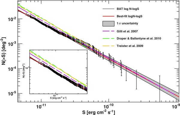
Figure 3. log N–logS of the BAT AGN (black data points) and best power-law fit in the 15–55 keV band. The shaded gray region represents the 1σ uncertainty computed via bootstrap. The dashed lines show the predictions of the number counts from the models of Gilli et al. (2007), Treister et al. (2009), and Draper & Ballantyne (2010). The inset shows a close-up view of the distribution at the lowest fluxes.
Download figure:
Standard image High-resolution imageIn order to compare our results with the log N–log S measurements published elsewhere, we adopt the following two strategies to convert fluxes from one band to another. In the first case, we adopt a simple power law with a photon index of 2.0 which is known to describe generally well the spectra of faint AGNs in the BAT band (Ajello et al. 2008b). Additionally, we use a more complex model for the AGN emission in the BAT band which is based on the PEXRAV model of Magdziarz & Zdziarski (1995). In Burlon et al. (2011), the stacking of ∼200 AGN spectra revealed that the average AGN spectrum is curved in the 15–200 keV band. This stacked AGN spectrum can be described using a PEXRAV model with a power-law index of 1.8, an energy cutoff of 300 keV and a reflection component due to a medium that covers an angle of 2π at the nuclear source (R ≈ 1 in the PEXRAV model). These parameters are reported in Table 1 of Burlon et al. (2011). To convert fluxes from the 15–55 keV band to the, e.g., 14–195 keV band used by Tueller et al. (2008), the two factors are 2.02 and 1.92 (for the power-law and PEXRAV model, respectively). So we consider the uncertainty related to the flux conversion to be of the ∼5% order.
We compare in Table 3 our results to those of Tueller et al. (2008), Cusumano et al. (2009), and Krivonos et al. (2010). When comparing INTEGRAL and BAT results, one has to take into account the different normalizations of the Crab spectrum that the two instruments adopt (Krivonos et al. 2010). To make a proper comparison, we convert the INTEGRAL 17–60 keV log N–log S to the 15–55 keV BAT band taking into account the different normalizations.6 It is apparent that there is excellent agreement with the results of Tueller et al. (2008), both in terms of the normalization of the log N–log S and also in terms of its slope. Both slopes reported by Cusumano et al. (2009) and Krivonos et al. (2010) are in agreement with ours, but the density of AGNs reported by Cusumano et al. (2009) is smaller than ours. We find an overall agreement within ∼10% of our results and the ones of Krivonos et al. (2010) as Figure 4 testifies.
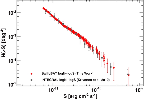
Figure 4. log N–logS of the BAT AGN in the 15–55 keV band (filled circles) compared to the one derived from INTEGRAL data by Krivonos et al. (2010) (squares).
Download figure:
Standard image High-resolution imageTable 3. Properties of log N–log S Derived above 10 keV
| Model | Surface Densitya | β |
|---|---|---|
| (10−3 deg−2) | ||
| This work | 6.67+0.11− 0.11 | 2.49+0.08− 0.07 |
| Tueller et al. (2008) | 6.5–6.8 | 2.42 ± 0.14 |
| Cusumano et al. (2009) | 5.4–5.9 | 2.56 ± 0.06 |
| Krivonos et al. (2010) | 7.0–8.1 | 2.56 ± 0.10 |
Note. aDensity at a 15–55 keV flux of 10−11 erg cm−2 s−1.
Download table as: ASCIITypeset image
We also compare the BAT results and the results of the population synthesis models of Gilli et al. (2007), Treister et al. (2009), and Draper & Ballantyne (2010). For both the Treister et al. and Draper & Ballantyne models, we used the predictions for the 10–30 keV band reported in Ballantyne et al. (2011) while for the Gilli et al. (2007) model we use the 10–40 keV predictions available online.7 Since BAT detects very few Compton-thick AGNs, we limited the predictions of the models of Gilli et al. (2007) and Draper & Ballantyne (2010) to objects with log NH ⩽ 24. The predictions by Treister et al. (2009) include objects with log NH ⩾ 24, however, in their modeling the density of Compton-thick AGNs is (at BAT sensitivities) ∼7% of the total AGN population. The predictions of all models, converted to the BAT band using the above prescriptions, are compared to the BAT log N–log S in Figure 3. It is apparent that there is good agreement with the BAT results at bright fluxes (i.e., > 10−11 erg cm−2 s−1). At the limiting flux of our analysis (i.e., ∼6 × 10⁻¹² erg cm−2 s−1), the model predictions are beyond the statistical uncertainty of the BAT log N–log S as shown in Table 4 and in the inset of Figure 3.
Table 4. Comparison of the BAT log N–log S with Synthesis Models
| Model | Surface Densitya |
|---|---|
| (10−2 deg−2) | |
| This work | 1.49+0.04− 0.03 |
| Gilli et al. (2007)b | 2.14–2.35 |
| Treister et al. (2009)c | 2.31–3.02 |
| Draper & Ballantyne (2010) | 2.52–3.20 |
Notes. aDensity at a 15–55 keV flux of 6× −12 erg cm−2 s−1. bTo convert the original 10–40 keV counts to the BAT 15–55 keV band, we have used the following factors: 0.94 and 1.04 for the power-law and PEXRAV model. cTo convert the 10–30 keV counts (reported in Ballantyne et al. 2011) to the BAT 15–55 keV band, we have used the following factors: 1.18 and 1.40 for the power-law and PEXRAV model.
Download table as: ASCIITypeset image
The model of Gilli et al. (2007) is compatible at bright fluxes with the BAT data, but with a steeper slope. On the other hand, there seems to be a constant offset between the BAT log N–logS and the model predictions of Treister et al. (2009) and Draper & Ballantyne (2010). The model of Treister et al. (2009) reproduces the 14–195 keV BAT log N–log S of Tueller et al. (2008) which is in very good agreement with the one published here. However, a close inspection (see Figure 1 in Treister et al. 2009) shows that the Tueller et al. (2008) data (reported in Treister et al. 2009) have a normalization ∼1.6 larger than the original measurement reported in Tueller et al. (2008). Thus, the Treister et al. (2009) is anchored to log N–logS data with a normalization ∼1.6 larger than observed. This same factor is apparent when comparing the Treister et al. (2009) prediction to our data (see Table 4).
The model of Draper & Ballantyne (2010) reproduces (see their Figure 3) the "correct" 14–195 keV log N–log S as reported by Tueller et al. (2008). However, their 10–30 keV model prediction is at fluxes ⩾10−14 erg cm−2 s−1 very similar to the one of Treister et al. (2009), and their predicted densities are a factor 1.6–1.8 larger than the measured ones in the 15–55 keV band (see Table 4) at the faintest fluxes sampled by our analysis. These findings might have some implications for the number of objects predicted to be detected by NuSTAR in serendipitous surveys above 10 keV (see Section 5). Given the substantial agreement of the BAT and INTEGRAL log N–log S (see Figure 4), it does not seem likely that the discrepancy in the predictions of synthesis models and the >10 keV log N–log S can be ascribed to a difference in the results above 10 keV.
3.2. The Luminosity Function
X-ray-selected (below 10 keV) AGNs are known to display an LF that evolves with redshift (see, e.g., Ueda et al. 2003; La Franca et al. 2005; Hasinger et al. 2005; Silverman et al. 2008; Aird et al. 2010). Our sample reaches a redshift of z ≈ 0.3 where according to the above works, the evolution of AGNs is significant and can potentially be detected. In Ajello et al. (2009a), we found marginal evidence for the evolution of AGNs in the local universe. Here, we can make use of our all-sky sample of Seyfert galaxies to test this hypothesis. We adopt as a description of the X-ray luminosity function (XLF) a pure luminosity evolution model as follows:
where V is comoving volume element and the evolution is parameterized using the common power-law evolutionary factor:

We neglect any cutoff in the evolution as this takes place at a redshift that BAT cannot constrain (i.e., z ≈ 1, see, e.g., Aird et al. 2010). For the XLF at redshift zero, we use a double power law of the form
A value of k significantly different than zero would point toward an evolution of the XLF. In order to derive the LF of AGNs, we adopt the same maximum likelihood method described in Ajello et al. (2009a). In particular, we determine the best-fit parameters of the XLF by finding the minimum of Equation (11) in Ajello et al. (2009a).
In order not to include sources which could have a nonnegligible contribution to their total luminosity from X-ray binaries (see, e.g., Voss & Ajello 2010) and to limit the incompleteness due to the bias against the detection of the most absorbed sources, we derive the XLF only for log LX ⩾ 41.3. The best-fit parameters for the Pure Luminosity Evolution (PLE) model in case of evolution (k ≠ 0) and in case of no evolution (k = 0) are reported in Table 5. The first result is that the model with no evolution (i.e., Equation (5)) represents a good description of the BAT data set. The best-fit parameters are compatible with those reported by Sazonov et al. (2008), Tueller et al. (2008), and Ajello et al. (2009a).
Table 5. Parameters of Fitted Luminosity Functions
| Model | Aa | γ1 | γ2 | L*b | k |
|---|---|---|---|---|---|
| No evolution | 113.1 ± 6.0a | 0.79 ± 0.08 | 2.39 ± 0.12 | 0.51 ± 0.14 | 0 |
| PLE | 109.6 ± 5.3a | 0.78 ± 0.07 | 2.60 ± 0.20 | 0.49 ± 0.10 | 1.38 ± 0.61 |
| No evolution, no CT | 122.4 ± 6.6a | 0.72 ± 0.09 | 2.37 ± 0.12 | 0.48 ± 0.13 | 0 |
Notes. Parameters without an error estimate were kept fixed during the fitting stage. aIn unit of 10−7 Mpc−3. bIn unit of 1044 erg s−1.
Download table as: ASCIITypeset image
Adding the extra k parameter produces only a marginal improvement in the fit. Indeed the log-likelihood improves only by ∼5 which corresponds to a ∼2σ improvement (Wilks 1938). This is reflected in the luminosity evolution parameter which is constrained to be k = 1.38 ± 0.61. The value found here is compatible, but smaller than the value of 2.62 ± 1.18 reported in Ajello et al. (2009a) showing that there is evolution in the XLF of local AGNs that might be shallower than previously found. We thus believe that the non-evolving XLF model is, in view of the marginal improvement of the goodness of fit, a better representation of the current data set. Nevertheless, we will use the PLE model in Section 5 to assess the level of uncertainty in the prediction for the number of AGNs that might be detected by NuSTAR in a very near future.
It is interesting to compare our XLF with that reported by Sazonov et al. (2008) and Tueller et al. (2008) in the 17–60 keV and in the 14–195 keV band, respectively. Sazonov et al. (2008) and Tueller et al. (2008) report a value of the faint-end slope γ1 of 0.76+0.18− 0.20 and 0.84+0.16− 0.22, respectively. The value of our faint-end slope is 0.78 ± 0.08 in agreement with both results, but much better constrained because of the larger data set. When converted to our band (see previous section for the conversion factors), the break luminosity of Sazonov et al. (2008) and Tueller et al. (2008) is, respectively, 2.2+2.0− 1.0 × 1043 erg s−1 and 3.7+3.0− 1.6 × 1043 erg s−1 while we measure 5.1 ± 1.4 × 1043 erg s−1 to be again compatible, but better constrained.
In order to display the LF, we rely on the "Nobs/Nmdl" method devised by La Franca & Cristiani (1997) and Miyaji et al. (2001) and employed in several recent works (e.g., La Franca et al. 2005; Hasinger et al. 2005). Once a best-fit function for the LF has been found, it is possible to determine the value of the observed LF in a given bin of luminosity and redshift:
where LX, i and zi are the luminosity and redshift of the ith bin, Φmdl(LX, i, zi) is the best-fit LF model and Nobsi and Nmdli are the observed and the predicted number of AGNs in that bin.
Figure 5 shows the best-fit non-evolving model (i.e., k = 0) in comparison with the XLF of Sazonov et al. (2008) and Tueller et al. (2008). In general, there is very good agreement between the XLFs derived in all of these works. Our results are also in agreement with those obtained in the <10 keV band. Indeed, for the bright-end slope Barger et al. (2005), La Franca et al. (2005), and Aird et al. (2010) obtain 2.2 ± 0.5, 2.36+0.13− 0.11, and 2.55 ± 0.12, respectively, while we measure 2.39 ± 0.12. For the faint-end slope, Barger et al. (2005), La Franca et al. (2005), and Aird et al. (2010) report 0.42 ± 0.06, 0.97+0.08− 0.07, and 0.58 ± 0.048 while we measure γ1 = 0.78 ± 0.08. The agreement for the faint-end slope is not as a good as for the bright-end slope and there is some scatter (that appears to be systematic in origin) in the <10 keV measurement while there is substantial agreement above 10 keV (see above discussion). An excessive flatness of the faint-end slope might be linked to the role of Compton-thick AGNs which are difficult to detect because the absorption pushes their observed luminosity below the survey threshold. Indeed, as shown in Burlon et al. (2011), 2–10 keV surveys are more biased in the detection of Compton-thick AGNs than surveys above 10 keV. Depending on the redshift distribution of the sources (and thus on the k-correction), the bias might not be the same for different 2–10 keV surveys.
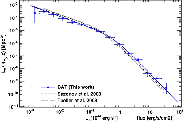
Figure 5. Luminosity function in the 15–55 keV band of the BAT AGN (non-evolving model) compared with the measurements of Tueller et al. (2008) and Sazonov et al. (2008). The data point at a luminosity < 2 × 1041 erg s−1 was not fitted to avoid problems related to incompleteness in detecting Compton-thick AGNs and to avoid contamination from sources whose flux might be dominated by the emission of X-ray binaries (Voss & Ajello 2010).
Download figure:
Standard image High-resolution imageFor completeness, we also report in Table 5 the best-fit parameters to the XLF of all AGNs, excluding the Compton-thick ones of Table 2. Because Compton-thick objects represent a small fraction of the AGNs detected by BAT, there is very little difference between the XLF of all AGNs and that of AGNs with log NH < 24. However, in the next section this XLF will be useful to compare the space density of Compton-thick AGNs to that of Compton-thin (log NH < 24) AGNs.
3.3. The Space Density of Compton-thick AGNs
We derive the space density of Compton-thick AGNs with 24 ⩽ log NH ⩽ 25 using the 1/VMAX non-parametric method (Schmidt 1968). We de-absorb the luminosities of the BAT Compton-thick sources reported in Table 2 using the correction function reported in (Burlon et al. 2011, see their Figure 11). This correction function was derived for the average properties of the Compton-thick AGN detected by BAT and takes into account photoelectric absorption as well as Compton scattering (see Murphy & Yaqoob 2009, for details).
Figure 6 shows the LF of the Compton-thick AGN detected by BAT while Figure 7 reports the cumulative space density. In this latter case, the uncertainty was computed via bootstrap with replacement. We find that the space density of Compton-thick AGNs with a de-absorbed luminosity greater than 2 × 1042 erg s−1 is 7.9+4.1− 2.9 × 10⁻⁵ Mpc−3. Above a de-absorbed luminosity of 1043 erg s−1 the density becomes 2.1+1.6− 1.4 × 10⁻⁵ Mpc−3. As shown in Figure 6, the model predictions of Gilli et al. (2007) are compatible within the statistical error with our space density estimates. Treister et al. (2009) and Draper & Ballantyne (2010) estimated a space density of log LX ⩾ 43 erg s−1 sources of, respectively, 2.2+2.9− 1.1 × 10⁻⁶ Mpc−3 and 3–7 × 10⁻⁶ Mpc−3. These estimate are below ours, but compatible within 2σ and 1σ, respectively.
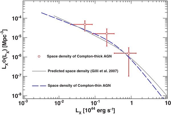
Figure 6. Space densities of Compton-thick AGNs detected by BAT compared to model prediction from Gilli et al. (2007) and the space density of Compton-thin (log NH < 24) AGNs from Section 3.2. Luminosities were de-absorbed following the method outlined in Burlon et al. (2011).
Download figure:
Standard image High-resolution image
Figure 7. Cumulative space densities of Compton-thick AGNs detected by BAT (thick red solid line) with 1σ confidence contours (dashed line) generated from the analysis of the bootstrapped samples (thin gray lines).
Download figure:
Standard image High-resolution imageIn the same Figure 6, we plot also the space density of AGNs with log NH < 24 (from the previous section). While there is substantial agreement between the two, our analysis seems to point to the fact that the space density of Compton-thick AGNs is larger than the one of all other classes of AGNs. By allowing the normalization A of the XLF of log NH < 24 AGNs to vary we find that  = 1.4
= 1.4 : i.e., the space density of Compton-thick AGNs is 1.4 times larger than that of log NH < 24 AGNs. A similar result was obtained by Della Ceca et al. (2008a) who derived indirectly the space density of Compton-thick AGNs as a difference between the density of optically selected AGNs and that of X-ray-selected AGNs with log NH < 24 (see the aforementioned paper for more details). In their study, they also find that the space density of Compton-thick AGNs with log LX ⩾ 43 erg s−1 is ∼1.6 × 10⁻⁵ Mpc−3 which is in good agreement with the value found here.
4. THE ANISOTROPIC LOCAL UNIVERSE
The BAT sample represents an incredible resource to study the properties of the nearby universe as it is a truly local sample of AGNs. Indeed, the median redshift of the radio-quiet AGNs detected by BAT is ∼0.03 which corresponds to ∼120 Mpc. On these scales, the structure of the local universe is known to be inhomogeneous and AGNs are known to trace the matter density distribution (Cappelluti et al. 2010). The BAT AGNs can thus be used to trace the large-local scale structure. Krivonos et al. (2007) reported, using 68 AGNs detected by INTEGRAL, an anisotropy of the spatial distribution of local AGNs. With an AGN sample ∼6 times larger than the INTEGRAL sample, it is possible to identify the anisotropic spatial distribution of AGNs to a higher precision than previously obtained.
The following approach is adopted in order to assess the anisotropy of the spatial distribution of AGNs. We first separate the sample into two redshift bins z < 0.02 and 0.02 ⩽ z ⩽ 0.15 corresponding to a distance smaller (or greater) than 85 Mpc. The choice is dictated by the fact that the largest contrast in AGN density is expected to be observed nearby from us.
For each of these sub-samples, we create a log N–log S that yields the average surface density of AGNs for that redshift slice. Taking into account how the BAT sensitivity varies across the sky, we generate (for each redshift bin) 1000 realizations of AGN sets which are isotropically distributed in the sky. Then, for each direction in the sky we count how many AGNs BAT has detected within a radius of 20° (typically this number oscillates around 10) versus the expected number for the isotropic case. For each of these sky positions, we compute the fractional overdensity of AGNs: i.e., the ratio between the number of detected AGNs and the number of expected objects if AGNs were isotropically distributed. From the 1000 realizations, we also compute the error (and the significance) connected to the fractional over-density.
Figures 8 and 9 show how the fractional overdensity of AGNs (i.e., the ratio of detected AGNs to the expected number for the isotropic case) and its significance change across the sky for the lower redshift bin. It is apparent that there is a marked contrast in the AGN density within 85 Mpc, with the AGN density varying by a factor of >10 across the sky. The most significant overdensity is seen in the first redshift slice (i.e., within 85 Mpc), with prominent structures significant at >4σ.
Figure 8. Fractional overdensity of AGNs with respect to the isotropic expectation within 85 Mpc. The color scale shows the ratio of BAT-detected AGNs (within 20°cones) to the average number of AGNs expected in the same area if sources were isotropically distributed. The map shows the regions where this ratio is the largest (red) and where it is the smallest (blue). The squares show the approximate position of the most prominent superclusters (see the text for details).
Download figure:
Standard image High-resolution image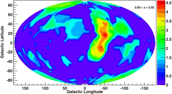
Figure 9. Significance of the density features of Figure 8 expressed in number of σ.
Download figure:
Standard image High-resolution imageThere is a clear overdensity of AGNs (a factor >4 larger than the isotropic expectation) in the direction of the super-galactic plane. In particular, the most dense region is found to be at l = −54° extending from b = ∼ 15° to b = ∼ 50°. This corresponds to the position of the Hydra–Centaurus supercluster (z = 0.01–0.02) which represents one of the largest structures in the local universe. The second most dense region (connecting to the south of the Hydra–Centaurus supercluster) can likely be identified with the "Great Attractor" (Lynden-Bell et al. 1988). In Figure 8, the positions of the Great Attractor, the Centaurus and Hydra superclusters, are shown with squares (from bottom left to upper right, respectively). The redshifts of the BAT AGN in these dense regions are in agreement with the redshifts of these massive structures. Our results appear to be in good agreement with the ones of Krivonos et al. (2007), but the improved statistics allow us to locate more precisely the overdensity of AGNs in the nearby universe.
In the 0.02 ⩽z ⩽ 0.15, the anisotropy is less pronounced and less significant as well, with the most significant structures being < 3σ. A comparison with our simulations (which allow us to account for the trial factor) shows that the 0.02 ⩽ z ⩽ 0.15 overdensity map is indistinguishable (with the present data) from the isotropic expectation. However, the local environment is known to be highly inhomogeneous up to (at least) z ≈ 0.05 (Jarrett 2004). The reason why BAT does not detect this anisotropy in the local scale structure is ultimately due to statistics. Indeed, the typical clustering length of the BAT AGN is known to be 5–8 Mpc (Cappelluti et al. 2010). Within 85 Mpc, our 20°search cone subtends9 a length of ∼16 Mpc which is comparable to the clustering length of AGNs. However, for the average redshift (∼0.05) of the 0.02 ⩽ z ⩽ 0.15 sample, the 20°search cone subtends a length of 70 Mpc which is 10 times larger than the typical clustering length of AGNs. This contributes to dilute any overdensity signal. In order to have a similar resolution to the <85 Mpc sample, one should adopt a search cone of 5°. However, with the current statistics we would expect less than 1 AGN in such cone.
Finally, we checked if the anisotropy depends on any of the AGN parameters (i.e., flux, luminosity, type, etc.). To this extent, we isolated the AGN in the direction of the Hydra–Centaurus superclusters and of the Great Attractor and created a log N–log S and an LF. The first result is that the XLF of these AGNs is in good agreement with that of the entire population reported in Figure 5. The log N–logS of the AGN in the direction of the superclusters is shown, in comparison with the log N–logS of the whole population, in Figure 10. It is clear that there is an excess at bright fluxes. This finding, in conjunction with the fact that the XLF does not change, indicates that the sources that contribute to the overdensity are the brightest sources (i.e., the proximity of these local structures makes these sources appear with a bright flux). Indeed, the median redshift of the AGN in the direction of the superclusters (z ≈ 0.015) is markedly smaller than that of the whole population (z ≈ 0.03).

Figure 10. log N–log S (15–55 keV) of the AGN in the direction of the Hydra–Centaurus superclusters and of the Great Attractor compared to the log N–log S of all AGNs.
Download figure:
Standard image High-resolution imageIt is also interesting to note that the fraction of Sy2 galaxies in the direction of the superclusters is larger than average. Indeed, the fraction of objects classified as Sy2 in our whole sample and in the sample of Cusumano et al. (2010) is ∼34% of the total AGN population. This ratio would increase to ∼45% if all the objects with no optical classification reported in this or the Cusumano et al. (2010) sample would be in reality Sy2s. While it is reasonable to expect that more than 50% of the objects lacking an optical classification are Sy2 galaxies, it is unlikely that all of them are Sy2s. So this represents an extreme scenario.
The fraction of Sy2 object becomes ∼50% if we consider only the AGN in the direction of the superclusters and increases to 58% ± 8% if we restrict to sources within 85 Mpc. This seems in agreement with what reported by Petrosian (1982) that Sy1s are more often found to be isolated than Sy2s. In dense environments, encounters between galaxies produce gravitational interactions that can trigger gas inflow toward the central hole and produce AGN activity. Galaxy merging is known to provide an efficient way to funnel a large amount of gas and dust to the central black hole (e.g., Kauffmann & Haehnelt 2000; Wyithe & Loeb 2003; Croton et al. 2006). Recently, Koss et al. (2010) found that 24% of all the hosts of the BAT-selected AGN have a companion galaxy within 30 kpc. This suggests that for a fraction of moderate luminosity AGN, merging is a viable triggering mechanisms. However, in dense environments major merging is not the only process that might be at work. Indeed, galaxy harassments (i.e., high speed encounters between galaxies) can also drive most of the galaxy's gas to the inner 500 pc (Lake et al. 1998) and thus trigger AGN activity. Also, minor merging, where the ratio of the masses of the merging galaxies is > 3 (and probably around ∼10), can lead to a Seyfert level of accretion (Hopkins & Hernquist 2009). With large quantities of gas available around the hole, in the early phase of accretion the AGN might have a higher probability of being identified as a type-2 AGN. This might explain the overabundance of Sy2 galaxies in dense environments.
5. PREDICTIONS FOR NuSTAR
In this section, we provide predictions for the number of objects that NuSTAR might see in different types of blank-field surveys. The predicted number counts are obtained by extrapolating the BAT log N–log S of Section 3.1 to lower fluxes under the assumption that the slope of the log N–log S does not change. Indeed, it is reasonable to expect so since there are strong indications both from observations in the 2–10 keV band and from modeling that the source count distribution breaks only at fluxes ⩽10−14 erg cm−2 s−1.
The source count distribution of AGNs is very well determined in the 2–10 keV band10 down to fluxes of <10−15 erg cm−2 s−1 (see, e.g., Rosati et al. 2002; Cappelluti et al. 2007; Xue et al. 2011). Its slope is known to be Euclidean down to fluxes of ∼10−14 erg cm−2 s−1. For example, Cappelluti et al. (2007) report that a slope of 2.43 ± 0.10 is in good agreement with our results. A similar result is found by Rosati et al. (2002). Also, population synthesis models predict a break in the log N–logS at < 10−14 erg cm−2 s−1 (Gilli et al. 2007; Treister et al. 2009; Draper & Ballantyne 2010).
The extrapolation to fluxes a factor >50 fainter than those sampled by BAT necessarily introduces some uncertainty related to neglecting the evolution of AGNs. This uncertainty will be gauged later on in this section. However, the fact that BAT and NuSTAR sample (almost) the same energy band removes other sources of uncertainties. NuSTAR will likely perform three different types of surveys: a shallow, a medium, and a deep survey. The shallow survey, performed combining short (5–10 ks) exposures, might extend over ∼3 deg2 reaching fluxes11∼10−13 erg cm−2 s−1. The medium survey will likely cover ∼1 deg2 with ∼50 ks pointings reaching a 10–30 keV flux of ∼ 5 × 10⁻¹⁴ erg cm−2 s−1 while the deep survey is expected to reach a 10–30 keV flux of ∼2 × 10⁻¹⁴ erg cm−2 s−1 (using 200 ks pointings) over an area of ∼0.3 deg2.
Ballantyne et al. (2011) reported the number of expected AGNs, in NuSTAR surveys, as predicted from different population synthesis models. Since the NuSTAR FOV is smaller than the surveyed area, NuSTAR will have to use a tiling strategy. Two tiling strategies can be foreseen: a corner-shift and half-shift survey (see also Ballantyne et al. 2011). In the corner-shift strategy, the survey area is covered by non-overlapping pointing. In the half-shift strategy, the distance between pointings is half the size of the FOV. The corner-shift strategy reaches deeper fluxes while the half-shift reaches a more uniform exposure of the surveyed area. Ballantyne et al. (2011) concluded that the half-shift strategy yields the larger number of AGNs. Thus, in order to make a proper comparison we adopt the sky coverages reported by Ballantyne et al. (2011) for the half-shift tiling strategy for the 10–30 keV band. Converting the sky coverages from the 10–30 keV to the 15–55 keV is rather easy and almost error free. Indeed, for the power-law and the PEXRAV model discussed in Section 3.1, we get a conversion factor of 1.16 and 1.18, respectively. Thus, using a log N–logS derived in an overlapping band reduces the uncertainties due to flux conversion to less than ∼2%.
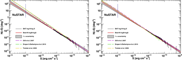
The numbers of objects predicted, extrapolating the log N–log S, for four different survey fields are reported in Table 6 and they are compared to the predictions of the models of Treister et al. (2009) and Draper & Ballantyne (2010) reported in Ballantyne et al. (2011). It is clear that our predictions lie substantially lower than the ones of population synthesis models. The left panel of Figure 11 shows that (at NuSTAR sensitivities) the predictions of synthesis models lie a factor ∼3 above the extrapolation of the log N–logS of BAT AGNs.
Figure 11. log N–logS of the BAT AGN (black data points) and best power-law fit extrapolated to the sensitivity that NuSTAR will achieve. The left panel shows the original prediction of synthesis models, while in the right panel the predictions have been renormalized to match the AGN densities measured by BAT. In both panels, the vertical dashed line shows the sensitivity reached by NuSTAR in a short pointing (i.e., 5–10 ks).
Download figure:
Standard image High-resolution image
Table 6. Predictions for NuSTAR Surveys Adopting the Half-shift Coverages Reported in Ballantyne et al. (2011)
| Model | BOÖTES | COSMOS | ECDFS | GOODS |
|---|---|---|---|---|
| (9.3 deg2) | (2 deg2) | (0.25 deg2) | (0.089 deg2) | |
| This work (no evolution) | 47+16− 13 | 31+13− 10 | 20+10− 7 | 16+8− 6 |
| Draper & Ballantyne (2010) | 126 | 91 | 62 | 51 |
| Treister et al. (2009) | 107 | 77 | 52 | 42 |
| Draper & Ballantyne (2010) | 66 | 46 | 31 | 26 |
| Treister et al. (2009) | 68 | 51 | 33 | 27 |
| Gilli et al. (2007) | 94 | 60 | 39 | 25 |
| This work (evolution) | 61 | 42 | 28 | 23 |
Notes. The lower part of the table shows the prediction of the models renormalized to match the BAT log N–log S.
Download table as: ASCIITypeset image
This disagreement is likely due to two reasons. Part of it is due to the fact that synthesis models lie systematically above the BAT log N–log S as shown in Section 3.1. The second one is that the simple extrapolation of the BAT log N–log S is not able to capture the evolution of AGNs, which is rather well established (e.g., Miyaji et al. 2001; La Franca et al. 2005; Hasinger et al. 2005) and expected also in the ⩾10 keV band.
In order to correct for the first problem (i.e., the overprediction of AGNs in the BAT band), we arbitrarily renormalize the models of Gilli et al. (2007), Treister et al. (2009), and Draper & Ballantyne (2010) to fit the BAT data at bright fluxes and then we convolve them with the same sky coverages described above. The predictions for the "renormalized" models are reported in the lower part of Table 6 and are on average compatible within ∼1σ with the extrapolation of the BAT log N–log S (as also visible in the right panel of Figure 11). This is reflected into a lower number of predicted AGN detections for NuSTAR in the 10–30 keV band.
In order to correct (or to gauge the uncertainty) due to neglecting any evolutionary effect in the log N–log S, we rely on the best-fit PLE model of Section 3.2. Even if marginally significant, we take the best-fit parameters at their face value and derive the number of expected objects in NuSTAR fields. These are reported in the last row of Table 6. As it can be seen, the predictions from the evolutionary XLF are in fairly good agreement with the predictions from the "normalized" synthesis models. We thus believe that this set of predictions (i.e., lower part of Table 6) for the number of AGNs detectable is realistic. However, the ultimate number of detected AGNs will likely depend on how the sensitivity will vary across the survey fields and, for the smallest fields, on cosmic variance.
6. SUMMARY AND CONCLUSIONS
The analysis presented here shows the power of an all-sky survey at hard X-rays to study the AGN in our local environment. Thanks to the large FOV and high sensitivity BAT has detected 428 AGNs all-sky above 10 keV with negligible (⩽5%) incompleteness. This represents the largest complete sample of AGNs detected so far. Below we summarize our findings.
- 1.The BAT AGN sample spans 10 decades in luminosity comprising objects detected at distance of ∼1 Mpc up to redshift ∼3.5. The AGN sample can be divided into objects whose emission is dominated by the accretion disk/corona (i.e., Seyfert galaxies) and jet-dominated sources (i.e., blazars and radio galaxies). Seyfert galaxies are detected at low redshifts and low luminosities, while jet-dominated sources that are ∼15% of the whole sample are detected at high luminosity and high redshift.
- 2.Samples of AGNs detected above 10 keV are instrumental to determine the size of the population of Compton-thick AGNs that are still detected in very small numbers. While a detailed measurement of the absorbing column density of all the AGNs in the BAT sample is left to a future publication, we cross-correlated our sample with known catalogs of bona fide Compton-thick AGNs. The BAT sample already comprises 15 (out of the 18 reported by Della Ceca et al. 2008b) bona fide Compton-thick AGNs and three likely candidates. The observed12 fraction of Compton-thick AGNs, relative to the whole population, is thus ∼5%. We showed that BAT will likely not detect the rest of the known candidate Compton-thick AGN. Since the BAT sensitivity still improves with time, future AGN samples detected by BAT will likely contain previously unstudied Compton-thick AGNs. A few (one or two objects) might be present already in this sample.
- 3.We performed a robust analysis, using bootstrapping, of the source counts distribution of the Seyfert-like objects detected by BAT. The BAT log N–log S is consistent with Euclidean down to the lowest fluxes spanned by this analysis (i.e., 6 × 10⁻¹² erg cm−2 s−1). The agreement between our and the INTEGRAL results (Krivonos et al. 2010) shows that the log N–log S of AGNs selected above 10 keV is established to a precision of 10%. The population synthesis models that we have tested (i.e., Gilli et al. 2007; Treister et al. 2009; Draper & Ballantyne 2010) are able to reproduce the BAT log N–log S at the brightest fluxes, but overestimate it at the lowest fluxes spanned by this analysis.
- 4.We derived the LF of (local) AGN and tested for its possible evolution with redshift. Even with our large sample of AGNs the evidence for the evolution of the XLF is at best marginal (i.e., ∼2σ). The BAT data are well described by a non-evolving XLF which is modeled as a standard double power law. We find that the slope of the faint end is γ1 = 0.79 ± 0.08 while that of the bright end is γ2 = 2.39 ± 0.12. These values are in good agreement with those of Sazonov et al. (2008) and Tueller et al. (2008), but better constrained. Given the small FOV, NuSTAR will not be able to directly constrain the properties of the low-luminosity low-redshift AGN. The BAT sample and the BAT XLF are thus instrumental to determine, in connection with the future NuSTAR samples, the evolution and growth of AGNs.
- 5.We derived the LF of Compton-thick AGNs and found that at redshift zero their space density is 7.9+4.1− 2.9 × 10⁻⁵ Mpc−3 for objects with a de-absorbed luminosity larger than 2 × 1042 erg s−1. Our measurement is slightly larger, but compatible within uncertainties, with the prediction of synthesis models.
- 6.The BAT samples of Seyfert galaxies are truly a local sample (median redshift 0.03) and can be used to study the spatial distribution of AGNs in the local universe. We detected significant overdensity features in the spatial distribution of AGNs located within 85 Mpc. The densest regions show a density of AGNs that is up to ∼5 times larger than the average all-sky density. These dense regions can be identified with the most prominent nearby superclusters: i.e., the Hydra–Centaurus supercluster and the "Great Attractor." The fraction of Sy2 galaxies (with respect to the total AGN population) appears to be larger than average in the direction of the overdense regions. This evidence might support an evolutionary link where close encounters of galaxies trigger AGN activity whose first appearance is obscured by dust and gas.
- 7.The BAT and the NuSTAR energy bands overlap and it is thus possible to derive straightforward predictions, from the log N–log S or the XLF, for the number of AGNs that NuSTAR might detect in survey fields in the near future. We find substantial agreement in the number of predicted objects if the predictions of population synthesis models are renormalized to match, at the lowest fluxes, the BAT log N–log S.
Owing to the capability of detecting the local (those within ∼200 Mpc), relatively low-luminosity AGNs, but also high-redshift blazars, the all-sky hard X-ray surveys—such as the Swift-BAT survey discussed in this paper—have the unique potential to study simultaneously both the nearby and the early universe. Such hard X-ray surveys represent a unique resource, since for many years, they will remain the most sensitive probes of the accretion history in the universe.
M.A. acknowledges extensive discussions with Nico Cappelluti. M.A. acknowledges Ezequiel Treister and David Ballantyne for making the predictions from their models available in a machine-readable format. The authors acknowledge the comments of the referee which helped improving this paper.
Facilities: Swift/BAT -
Footnotes
- 5
1 mCrab in the 15–55 keV band corresponds to 1.27 × 10⁻¹¹ erg cm−2 s−1.
- 6
In order to convert the INTEGRAL data to the BAT band, we took into account that 1 BAT-mCrab in the 17–60 keV band is 1.22 × 10⁻¹¹ erg cm−2 s−1 while 1 INTEGRAL-mCrab is 1.43 × 10⁻¹¹ erg cm−2 s−1. Sub-sequently, we converted the 17–60 keV fluxes to the 15–55 keV adopting a power law with an index of 2.0. This leads to FBAT15 − 55 = 0.878 FINTEGRAL17 − 60.
- 7
The Gilli et al. (2007) model is available at http://www.bo.astro.it/~gilli/counts.html
- 8
Aird et al. (2010) also report 0.70 ± 0.03 for their PLE model.
- 9
The average redshift of the z < 0.02 sample is 0.01.
- 10
For a typical AGN spectrum, the 2–10 keV flux is on average 20% larger than the 15–55 keV flux.
- 11
Typical fluxes for NuSTAR are quoted for the 10–30 keV band. Here, we have converted those fluxes to the 15–55 keV band adopting a power law with a photon index of 2.0.
- 12
See Burlon et al. (2011) for the bias that instruments above 10 keV also have in detecting Compton-thick AGNs.