


ABSTRACT
Despite significant progress in understanding the dynamics of the corona, there remain several unanswered questions about the basic physical properties of coronal loops. Recent observations from different instruments have yielded contradictory results about some characteristics of coronal loops, specifically as to whether the observed loops are spatially resolved. In this paper, we examine the evolution of coronal loops through two extreme-ultraviolet filters and determine if they evolve as a single cooling strand. We measure the temporal evolution of eight active region loops previously studied and found to be isothermal and resolved by Aschwanden & Nightingale. All eight loops appear in "hotter" TRACE filter images (Fe xii 195 Å) before appearing in the "cooler" (Fe ix/Fe x 171 Å) TRACE filter images. We use the measured delay between the two filters to calculate a cooling time and then determine if that cooling time is consistent with the observed lifetime of the loop. We do this twice: once when the loop appears (rise phase) and once when it disappears (decay phase). We find that only one loop appears consistent with a single cooling strand and hence could be considered to be resolved by TRACE. For the remaining seven loops, their observed lifetimes are longer than expected for a single cooling strand. We suggest that these loops could be formed of multiple cooling strands, each at a different temperature. These findings indicate that the majority of loops observed by TRACE are unresolved.
Export citation and abstract BibTeX RIS
1. INTRODUCTION
Recently, there has been significant debate over whether solar coronal loops observed with current instruments are resolved (Reale & Peres 2000; Schmelz et al. 2001; Testa et al. 2002; Del Zanna & Mason 2003; Aschwanden & Nightingale 2005; Cirtain et al. 2007; Aschwanden & Boerner 2011). Resolving a coronal loop requires that the width of the structure be larger than the resolution of the instrument and that the temperature at a single point along the structure be isothermal. If, instead, the loop is not consistent with a single temperature (i.e., the loop is multi-thermal), the loop is thought to be composed of several unresolved strands. We use the term "strand" for the largest magnetic flux tube on which the plasma's properties, such as density and temperature, are uniform on the cross section, and the term "loop" for an identifiable coherent structure in an observation. Based on these definitions, if the loop is resolved, it is formed of a single strand.
One technique that has been commonly employed to investigate the temperature structure of coronal loops is determining the differential emission measure (DEM) distribution. If the DEM is very narrow, the plasma is considered to be isothermal; if it is broad, the plasma is multi-thermal. DEM distributions can be determined from spectral observations or multiple filter observations. Several studies have found evidence for broad temperature distributions in coronal loops (e.g., Kano & Tsuneta 1996; Schmelz et al. 2001; Schmelz 2002; Martens et al. 2002) using spectral line observation from the Solar and Heliospheric Observatory (SOHO) Coronal Diagnostics Spectrometer (CDS) with 4'' pixel−1 resolution and analysis of data from the Soft X-ray Telescope (SXT) on Yohkoh with ∼2 5 pixel−1 resolution. New observations from the extreme-ultraviolet (EUV) Imaging Spectrometer (EIS) on Hinode, capable of observing active regions over a wide range of temperatures at relatively high spatial resolution (1'' pixel−1), have shown that some isolated coronal loops that are bright in Fe xii have narrow temperature distributions, but are not isothermal (Warren et al. 2008).
In contrast, Aschwanden & Nightingale (2005) presented a quantitative analysis of the thermal structure of coronal loops using a set of 234 thin loops observed with the Transition Region and Coronal Explorer (TRACE) with 05 pixel−1 resolution. They found the vast majority (84%) of the acceptable DEM fits to be isothermal, thereby concluding that TRACE was resolving "monolithic" loops, i.e., single temperature strands with widths of ≈ 14–28. Furthermore, a detailed study of a single loop by Del Zanna & Mason (2003) with both TRACE and SOHO CDS has shown isothermal cross-sectional temperatures of T0.7– 1.1 MK; however, the measured widths (8'') were significantly larger than loop strand widths measured by Aschwanden & Nightingale (2005).
To summarize, lower resolution (⩾1'' pixel−1) observations tend to find multi-thermal loops, while the high-resolution observations (05 pixel−1) find primarily isothermal solutions. These results would indicate that the high-resolution observations are indeed resolving solar coronal loops. Unfortunately, one limitation of the observational results from TRACE is that they are derived from only three narrowband filters (Fe ix/x, Fe xii, and Fe xv), and thus the temperature range of the inferred DEMs is limited to Te ≈ 0.7–2.7. This makes it difficult to eliminate the possibility of a multi-thermal DEM.
An additional observational characteristic of the EUV loops observed with TRACE is that they evolve, i.e., they first appear in the hotter TRACE filters and later appear in the cooler TRACE filter (Winebarger et al. 2003). Using the delay in the loop's appearance to calculate a cooling time, Winebarger et al. (2003) found that four of the five loops' lifetimes were larger than expected for the calculated cooling time, indicating that the loops were not simple cooling strands. Warren et al. (2003) simulated one of the loops and found the observational properties of the loops could be explained as a bundle of evolving sub-resolution strands, similar to a short-lived "nanoflare" storm (Cargill 1994; Klimchuk & Cargill 2001).
In this paper, we will use the loop's evolution to address the debate of whether coronal loops are resolved by TRACE. We will answer the question: Do the loops classified as isothermal by Aschwanden & Nightingale (2005) evolve like single strands? We choose eight well-observed loops from the Aschwanden & Nightingale (2005) study. Similar to Winebarger et al. (2003), we use the delay in a loop's appearance and disappearance in the series of filters to calculate cooling times and then determine if the cooling times are consistent with the observed lifetime of the loop. If the calculated lifetimes are approximately equal to the measured lifetimes, we conclude that the loop could consist of a single strand.
We find that only one of the eight loops has an evolution consistent with a single cooling strand. The evolutions of the remaining seven loops are inconsistent with a single cooling strand; their lifetimes are longer than expected. We suggest that these loops could be consistent with a multi-strand loop, with each strand at a different temperature. This would imply that the majority of loops observed with TRACE are not spatially resolved. We discuss other possible explanations of this result in Section 4.
2. THEORY
Previous analyses have shown that EUV loops observed with TRACE evolve; i.e., they "appear" in filters sensitive to hotter plasma before appearing in filters sensitive to cooler plasma (Warren et al. 2003; Winebarger et al. 2003). If the loop is a single cooling strand, then the appearance times of the loop in different filters as well as the loop's lifetime in a given filter are all determined by a single cooling time. In this section, we discuss how we calculate the cooling time from the observed light curve and predict the expected lifetime from the observed evolution of a loop in multiple TRACE filters.
We first assume that the plasma temperature falls off exponentially as it evolves; i.e.,
where T0 is the initial temperature of the plasma and γT is the cooling time. Furthermore, we assume that the cooling time and the density (which evolves more slowly than the temperature) are constant as the plasma cools through the temperatures at which the TRACE passbands are most sensitive. The left panel of Figure 1 shows an example of the expected temperature evolution of the plasma. For this example, the initial temperature, T0, was assumed to be 3 MK and the cooling time, γT, was assumed to be 1200 s. Here, it is important to note that γT is a phenomenological description of the cooling (after the heating is turned off) and would characterize conductive and radiative cooling. It is not the solution to a one-dimensional hydrodynamic model.
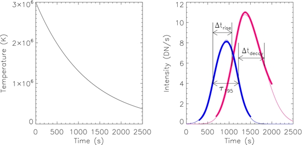
Figure 1. Left panel: the assumed evolution of temperature for a hypothetical plasma shown as a function of time. Right panel: the predicted intensities of the loop in the 195 Å filter (blue, left peak) and the 171 Å filter (pink, right peak) as a function of time. The solid lines tracing the light curves are asymmetric Gaussian fits to each light curve. The delays between the 195 and 171 Å light curves are measured during both the rise and decay phases. The lifetime of the loop in the 195 Å filter is also shown.
Download figure:
Standard image High-resolution imageBy convolving this temperature evolution with the TRACE temperature response functions and assuming a density (ne = 109 cm−3), we predict the expected intensity in the 195 Å (blue) and 171 Å (pink) filters as a function of time, shown in the right panel of Figure 1. The thick lines are Gaussian fits to each light curve. Visual inspection of the light curves indicates a clear delay in the appearance and disappearance of the loop in the subsequent filters. The loop appears in the 195 Å at approximately 300 s into the simulation. Then, from 700 to 2100 s the loop appears and disappears in the 171 Å channel. Here, we define the appearance and disappearance of the loop in a given filter as when the intensity of the loops becomes greater or less than half the maximum intensity, respectively. We term the delay between these appearance times Δtrise and the delay between the disappearance times Δtdecay. The lifetime of a loop, τ, is the difference between the appearance and disappearance times in a single filter. These values are shown graphically in Figure 1. Below we calculate the relationships between the delay times, the cooling time, and the expected lifetimes.
Using Equation (1), one can find the time it takes for the plasma to cool from one temperature to another, i.e.,
Hence, if this delay time is measured and the two temperatures are known, one can solve for the cooling time, i.e.,
To calculate the cooling time from the TRACE light curves, we must first determine the temperature sensitivity of the TRACE filters. For instance, we must determine what temperature the plasma must be before it appears in the TRACE 195 Å filter. To determine these temperatures, we use the simplification of the TRACE filter response functions provided by Warren et al. (2003), who assumed the filter response functions are well approximated by Gaussian functions. The 171 Å filter peaks at T171 = 9.6 × 10⁵ K and has a width of σ171 = 2.5 × 10⁵ K, while the 195 Å filter peaks at T195 = 1.4 × 10⁶ K and has a width of σ195 = 2.8 × 10⁵ K. To be consistent with the definition that the loop appears when the intensity becomes greater than half the maximum intensity, we choose that the temperature regime of a filter is defined as the full width at half-maximum (FWHM) of the filter response function. Furthermore, to limit the temperature range under consideration, we only consider the relationship between the delay in the appearance during the rise and decay phase of the loop between the 195 and 171 Å filter images and the lifetime in the 195 Å filter.
The cooling time can then be estimated from the measured delays between the 195 to 171 Å filters during both the rise phase (Δtrise) and the decay phase (Δtdecay) by combining Equation (3) with the filter response information, i.e.,

Similarly, for the decay phase, the cooling time (γT) is

Combining these cooling times and the filter response information with Equation (2), we can then predict the expected lifetime of the loop in the 195 Å filter,

Above, we have derived relationships that relate the observed delay in appearance of a loop in multiple EUV filters to the cooling time and expected lifetime of the loop. Here, we demonstrate the expected accuracy of this method using the example loop shown in Figure 1. The delay is measured on both the rise phase and the decay phase of the light curves. The measured delay on the rise phase (Δtrise) is 407 s and the delay on the decay phase (Δtdecay) is equal to 626 s. Using these delays in Equations (5) and (7), we estimate a cooling time (γT) of 1262 s during the rise phase and 1315 s during the decay phase. From Equation (9), the calculated lifetimes of the loop (τ195calc) are 617 s and 644 s for the rise and decay phases, respectively. The observed lifetime of the loop calculated as the FWHM of the fit to the 195 Å light curve, τ195meas, is 604 s.
In the example, the calculated cooling times (1262 s and 1315 s) were within 10% of the actual cooling time (1200 s). The calculated lifetimes (617 s and 644 s) were within 7% of the observed lifetime (604 s), confirming that a single strand was modeled. The best possible accuracy of this method, then, is 10%, which does not take into account errors associated with measuring the light curve or the systematic error that is introduced by assuming the density is constant. If, in the observations, the observed lifetime is within 10% of the calculated lifetime, we conclude that the loop is evolving as a single strand.
3. DATA AND ANALYSIS
The loops considered in this study were selected from the 234 thin coronal loops that have been previously analyzed by Aschwanden & Nightingale (2005). The candidate coronal loops were observed with TRACE. The details of the instrument have been described by Handy et al. (1999), Schrijver et al. (1999), and Golub et al. (1999). We first determine if there was adequate data coverage for the active region loops 1 hr before and after the Aschwanden & Nightingale (2005) image times. For each data set with adequate time coverage, we evaluated each loop to see if it remained unobscured by other structures during its evolution. Eight secluded loops with excellent time coverage were selected; all eight loops were found to be isothermal by Aschwanden & Nightingale (2005).
Figure 2 shows the selected loops, which were observed with TRACE on 1999 August 9 and 1999 November 6. The eight selected loops in TRACE 171 Å filter images are shown in the left column of Figure 2. These images were then smoothed with a boxcar smoothing function 7 pixels wide. The smoothed image was subtracted from the original image; the result is shown in the right column of Figure 2. The loops appear sharper in the manipulated image. The solid lines in the figures outline the loops and the area considered for background subtraction. Additional information such as the dates of observation, the loop lengths and widths are given in Table 1. The listed loop lengths and widths in Table 1 are measurements from Aschwanden & Nightingale (2005).

Figure 2. TRACE 171 Å images of the selected loops (left panels) and smoothed images subtracted from real images of the selected loops (right panels). The solid lines outline the loops and the area considered for background subtraction.
Download figure:
Standard image High-resolution imageTable 1. Loop Information
| Loop | Observation Date | Time | Half Loop Length | Width |
|---|---|---|---|---|
| (s) | (Mm) | (Mm) | ||
| 1 | 1999 Aug 9 | 16:30:41 | 75.1 | 1.41 ± 0.31 |
| 2 | 1999 Aug 9 | 19:35:29 | 92.3 | 1.42 ± 0.26 |
| 3 | 1999 Aug 9 | 19:35:29 | 157.6 | 1.50 ± 0.25 |
| 4 | 1999 Aug 9 | 22:15:02 | 240.0 | 1.46 ± 0.20 |
| 5 | 1999 Aug 9 | 22:15:02 | 237.6 | 1.45 ± 0.33 |
| 6 | 1999 Aug 9 | 22:15:02 | 145.9 | 1.51 ± 0.26 |
| 7 | 1999 Nov 6 | 02:52:40 | 97.7 | 1.29 ± 0.29 |
| 8 | 1999 Nov 6 | 02:52:40 | 227.4 | 1.29 ± 0.22 |
Download table as: ASCIITypeset image
To carefully calculate and subtract background, we have used the same methods as of Winebarger et al. (2003). We extract the loop pixels from the original image (i.e., the pixels between the lines outlining the loops in Figure 2) so that the loop runs through the center of a rectangular image. We then remove the loop from the rectangular image and fill the vacant pixels with interpolated data points found by fitting a linear function to the intensity of the background pixels on either side of the loop. Next, we smooth the background image and subtract it from the original image. The subtracted image is then used as a best estimate of the background subtracted loop. The error in the remaining intensity in a single pixel of the subtracted image is due to both Poisson statistics and the uncertainty associated with background subtraction. The uncertainty due to Poisson statistics is the square root of the total intensity in the pixel divided by the square root of the gain of the TRACE CCD. We take the standard deviation of the intensity of the pixels used to calculate the background as the uncertainty from background subtraction.
For each loop, we select a well-isolated region of the loop and sum all the pixels in that region to get a single intensity at that image time. We complete this analysis for each image in our data set to determine the intensity of each loop in each filter as a function of time. The resulting light curves are shown in Figure 3 as points with error bars. The intensities of the loops in the 195 Å are shown in blue and in the 171 Å are shown in pink. We then fit these light curves with asymmetric Gaussian functions, i.e., we allow the width of the Gaussian to be different on either side of the average value. The fits are shown in Figure 3 as solid lines.
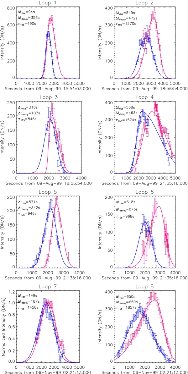
Figure 3. Light curves of the loops in the 195 Å (blue) and 171 Å (pink) bandpasses are shown. The light curves show evidence of a delay during the rise and decay phases of the loops. The solid lines are Gaussian fits to each light curve. The error bars show uncertainty in the intensity measurements.
Download figure:
Standard image High-resolution imageUsing the Gaussian fits, we measure the delays, i.e., the lag in appearance or disappearance of the loop in subsequent filters, in both the rise and decay phases. We also measure the FWHM of the Gaussian fits to determine the lifetime of the loop in the 195 Å filter. These values are given in Table 2 for the rise phase and in Table 3 for the decay phase of the loops. The errors in delay and lifetime measurements include errors from uncertainty in the intensity measurements and errors from the Gaussian fit of the light curves.
Table 2. Measured Rise Delays, Cooling Times, Measured and Calculated Lifetimes of the Selected Loops
| Loop | Δtrise | γT | τ195meas | τ195calc | Ratio | Single or Multi |
|---|---|---|---|---|---|---|
| (s) | (s) | (s) | (s) | |||
| 1 | 94 ± 17 | 291 ± 52 | 490 ± 83 | 143 ± 26 | 3.4 ± 0.2 | M |
| 2 | 549 ± 36 | 1702 ± 113 | 1270 ± 87 | 834 ± 55 | 1.5 ± 0.1 | M |
| 3 | 316 ± 74 | 977 ± 231 | 846 ± 59 | 480 ± 113 | 1.8 ± 0.2 | M |
| 4 | 538 ± 51 | 1668 ± 158 | 1574 ± 72 | 817 ± 78 | 1.9 ± 0.1 | M |
| 5 | 571 ± 47 | 1770 ± 146 | 946 ± 49 | 867 ± 72 | 1.1 ± 0.1 | S |
| 6 | 618 ± 112 | 1916 ± 347 | 968 ± 57 | 1034 ± 170 | 0.9 ± 0.2 | S |
| 7 | 149 ± 78 | 462 ± 158 | 1450 ± 82 | 226 ± 119 | 6.4 ± 0.5 | M |
| 8 | 650 ± 47 | 2015 ± 146 | 1857 ± 69 | 987 ± 126 | 1.9 ± 0.1 | M |
Download table as: ASCIITypeset image
Table 3. Measured Decay Delays, Cooling Times, Measured and Calculated Lifetimes of the Selected Loops
| Loop | Δtdecay | γT | τ195meas | τ195calc | Ratio | Single or Multi |
|---|---|---|---|---|---|---|
| (s) | (s) | (s) | (s) | |||
| 1 | 356 ± 21 | 748 ± 58 | 490 ± 83 | 367 ± 32 | 1.3 ± 0.2 | M |
| 2 | 472 ± 42 | 991 ± 123 | 1270 ± 87 | 486 ± 65 | 2.6 ± 0.2 | M |
| 3 | 107 ± 55 | 225 ± 212 | 846 ± 59 | 110 ± 119 | 7.7 ± 1.1 | M |
| 4 | 463 ± 33 | 972 ± 133 | 1574 ± 72 | 476 ± 83 | 3.3 ± 0.2 | M |
| 5 | 342 ± 37 | 718 ± 137 | 946 ± 49 | 352 ± 69 | 2.7 ± 0.2 | M |
| 6 | 875 ± 106 | 1838 ± 316 | 968 ± 57 | 901 ± 165 | 1.1 ± 0.2 | S |
| 7 | 187 ± 67 | 393 ± 148 | 1450 ± 82 | 193 ± 107 | 7.5 ± 0.6 | M |
| 8 | 669 ± 34 | 1405 ± 136 | 1857 ± 69 | 688 ± 113 | 2.7 ± 0.2 | M |
Download table as: ASCIITypeset image
Using Equations (5) and (7), we calculate a cooling time during the rise and decay phases for each loop; these are given in Tables 2 and 3. From the cooling time, we then calculate the expected lifetime of the loops in the 195 Å filter. The expected 195 Å lifetimes and errors are also given in Tables 2 and 3.
From Table 2, the observed lifetimes for Loops 5 and 6 are within 10% of the calculated lifetimes from the rise phase, while from Table 3, only Loop 6 has a observed lifetime approximately equal to the calculated lifetime from the decay phase. We conclude that only Loop 6 is evolving as expected for a single cooling strand which, in a single image, would appear isothermal. The isothermality of Loop 6 agrees with the findings of Aschwanden & Nightingale (2005).
The remainder of the loops, however, have observed lifetimes longer than calculated from the cooling times. The range of the ratio of the observed to calculated lifetimes is 1.3–7.7, meaning loops may be bright in a filter almost eight times longer than expected for a single cooling strand. These loops may indeed be bundles of unresolved strands; we discuss this and other possible explanations in the following section.
4. DISCUSSION
In this study, we have addressed one of the central questions for current instrumentation: Are we resolving coronal loops? We have utilized the temporal evolution of TRACE EUV coronal loops to determine their potential substructure. We selected eight isolated loops that were previously studied and found to be resolved and isothermal by Aschwanden & Nightingale (2005). For each of the eight loops, we have calculated the TRACE 195 and 171 Å intensities as a function of time and determined the delay between the light curves during the rise and decay phase of their evolution. This delay is an important property of the observed light curves as it constrains the loops' cooling time.
Using the calculated delays, we estimated cooling times and calculated an expected lifetime in the 195 Å filter for each loop. If the measured lifetime and expected lifetime were within 10% of one another, we concluded that the loop is evolving as a monolithic structure with uniform temperature over the cross section. One of the eight loops, Loop 6, met this criteria, with the ratio of its measured lifetime to calculated lifetime approximately equal to one as shown in Tables 2 and 3. Loop 6 evolves as a single strand during both the decay and rise phases during this observation time. The remainder of the loops had observed lifetimes longer than predicted. These loops are not easily modeled as a single cooling strand. These results did not agree with the conclusions of Aschwanden & Nightingale (2005).
The results presented in this paper are consistent with the results presented in Winebarger et al. (2003). In that paper, they found only one of the five analyzed loops to have an observed lifetime consistent with the expected lifetime. The remaining four loops had observed lifetimes 2–4 times longer than expected. Unlike the eight loops presented in this paper, however, there was no additional analysis to assess whether the loops appeared to be isothermal in a single image or not.
One explanation for the long observed lifetime is that the loop is formed of a bundle of sub-resolution strands, each heated impulsively at different times and to different temperatures and cooling independently. Such a model has long been thought to represent a short nanoflare storm (Cargill 1994). Warren et al. (2003) demonstrated that such a model could match the observed long lifetimes of TRACE loops. However, there are several additional potential explanations for the longer lifetime. For instance, the strands that form the loop could be re-heated during their evolution. Such an event would prolong their observed lifetime (Jakimiec et al. 1992; Reale 2007). The re-heating event, however, would have to occur after the strand cooled into the 195 Å filter; if it occurred before, it would affect both the delay and the lifetime.
Background subtraction could also play a role in the measurement of the appearance and disappearance times; other methods of background subtraction (see Terzo & Reale 2010) may provide different results. Other structures in the fore or background could be brightening during the loop's evolution. The TRACE images in Figure 2 illustrate the difficulty of extracting information about the temporal properties of the loops. Despite the fact that the selected loops are thin and somewhat spatially isolated, other structures may still manage to overlap with the selected section of the loop during these observations.
In this paper, we calculated the cooling times of the loops during both the rise and decay phase. A comparison of the cooling times is shown in Figure 4. The broken line shows where the cooling times during the rise and decay phase are equal. Loops 6 and 7 have similar cooling times during both phases and so lie on this line. Almost all of the loops have longer cooling times during the rise phase. This is consistent with the findings of Warren et al. (2003), and demonstrates that magnitude of the energy input is different during each phase.
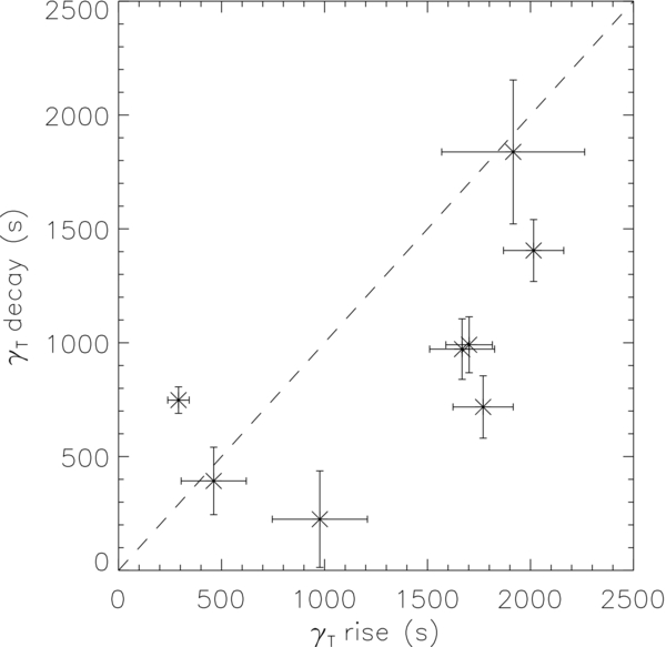
Figure 4. Relationship between the cooling time of the eight loops measured during the rise phase and cooling time measured during the decay phase is shown. Majority of the loops have longer cooling times during their rise phase. The broken line shows where the cooling times during the rise and decay phases are approximately equal.
Download figure:
Standard image High-resolution imageIn this study, we assumed that the temperature of the observed loops was decaying exponentially and the density and cooling time of the loops were constant. These assumptions were necessary to demonstrate the inconsistency between the observed and predicted lifetimes. However, these assumptions are extreme simplifications of the actual evolution of the plasma. Indeed, the density of the plasma may be evolving dramatically during this time (see the previous studies by Serio et al. 1991; Jakimiec et al. 1992; Bradshaw & Cargill 2005, 2010 that have demonstrated the important n∝Tδ relationship between temperature and density). In a subsequent paper, we will present simulations (similar to those performed by Warren et al. 2003) of representative loops to demonstrate if the loops can be modeled as a set of small-scale, impulsively heated filaments and reproduce the spatial and temporal properties of the observed loop.
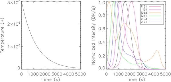
One limitation of the observational results from TRACE is that they are derived from only three narrowband filters (Fe ix/x, Fe xii, and Fe xv). NASA's mission to study the Sun, the Solar Dynamics Observatory/Atmospheric Imaging Assembly (AIA), now provides high-resolution, full Sun observations over a wide temperature range and rapid sequences. For example, the left panel of Figure 5 shows a possible evolution of a hypothetical cooling loop with constant density. The right panel of Figure 5 shows the expected evolution of the loop through six AIA channels. The multiple channels of AIA provide a unique opportunity to measure the evolution of individual loops to better understand their properties.
Figure 5. Left panel: the assumed evolution of temperature for a hypothetical cooling loop shown as a function of time. Right panel: the predicted evolution through the AIA filters. Some AIA channels are double peaked because the bandpass contains both hot and cool lines.
Download figure:
Standard image High-resolution image
TRACE is supported by contract NAS 5-38099 from NASA to LMATC. This work has been funded by Dr. Amy Winebarger's NSF Career Grant, the NSF Center for Integrated Space Weather Modeling (CISM), and NASA's Postdoctoral Program. The authors thank the NPP host facility, Marshall Space Flight Center, and Oak Ridge Associated Universities (ORAU). The authors are also grateful to the referee for providing helpful comments on the manuscript.