


ABSTRACT
Three-dimensional resistive magnetohydrodynamic simulations of the magnetic interaction of extrasolar planets with their host stars are performed on the basis of a Weber–Davis model of stellar winds. The free parameters of this model are the stellar magnetic field, the temperature of the corona, and the mass flux and have been fitted in order to theoretically explain the observed phase shifts between the so-called hot spots in the stellar chromospheres and the substellar points for the planets HD 179949 b and υ And b. The relative motion between planet and stellar wind causes perturbations of the stellar magnetic field, which propagate along the Alfvén characteristics toward the star. In a first step it is investigated whether the planet has to be magnetized in order to perturb the magnetic field. The second step consists of time-dependent simulations of the propagation, where the component of the electric current density parallel to the magnetic field is used to trace the perturbation. The simulations confirm the theoretical model for the explanation of the observed phase shifts for both planets.
Export citation and abstract BibTeX RIS
1. INTRODUCTION
One of the most interesting differences between numerous extrasolar planetary systems and the solar system is the close proximity between star and planet(s): about 100 of the more than 500 extrasolar planets discovered so far are so-called hot Jupiters, i.e., planets of the size of Jupiter on orbits closer than that of Mercury, partially even less that 10 stellar radii. While the solar system planets simply react to the inflowing solar wind, hot Jupiters being very close-in are mutually interacting with their host stars. The transition between these two scenarios takes place at the Alfvén radius, where the stellar wind velocity reaches the local Alfvén speed (e.g., Zarka et al. 2001). Possible interaction scenarios were discussed by Cuntz et al. (2000) and Cuntz & Shkolnik (2002), suggesting that a magnetic interaction should lead to an enhanced stellar activity. Such a behavior was actually observed by Shkolnik et al. (2003) and Shkolnik et al. (2005) at the stars HD 179949 and υ And, respectively, which was also interpreted as an indication for a planetary magnetic field. A remarkable feature of these observations was a significant phase shift between a so-called hot spot of the chromospheric activity and the substellar point. The measured phase shifts are 60° for HD 179949 b and even 169° for υ And b. More recent observations indicate such phase-shifted points of stellar activity also for the stars HD 189733, HD 192263, and τ Boo (e.g., Lanza 2008, 2009). As shown by Shkolnik et al. (2008) these events cannot be seen at all times, but their occurrence appears to depend on stellar activity cycles or changes in the structure of the stellar magnetic field structure.
As a first theoretical explanation of these phase shifts, McIvor et al. (2006) suggested the hot spot to be caused by particle acceleration along the magnetic field in consequence of magnetic reconnection. They used a tilted dipole field that becomes radial beyond the source surface for the stellar magnetic field. With such a field they could explain the phase shift for HD 179949 b, but failed for υ And b, because the model does not permit phase shifts beyond 90°. Numerical simulations by Cohen et al. (2009) showed that more realistic stellar magnetic fields, e.g., adopted measurements for the active Sun, may lead to large phase shifts. Preusse et al. (2006) suggested that, similar to the Io–Jupiter scenario, the relative motion between the (conducting) planet and the stellar wind causes perturbations of the stellar magnetic field, which propagate along Alfvén characteristics toward the star, while the planet moves along its orbit. The magnetic field here is that of the Weber–Davis model (Weber & Davis 1967) which is continued up to the stellar corona, i.e., a special magnetic topology within the source surface is not taken into account; consistent with McIvor et al. (2006), the hot spot itself may be caused by particles accelerated by electric fields parallel to the magnetic field by magnetic reconnection (Kopp et al. 1998). The model by Lanza (2008) is based on the model by McIvor et al. (2006), but constructs a linear force-free coronal magnetic field, based on a model by Neukirch (1995). This model includes a toroidal magnetic field being scaled with a parameter α, but is valid only within a certain distance form the star. With the model by Lanza (2008) the observed phase can be fitted for all stars mentioned above with a negative value for α, except for HD 192263 b, where a positive value is needed. This model also takes into account energetic considerations (Lanza 2009), which, however, are beyond the scope of the present study. The above-mentioned on-and-off nature of the planet–star interaction as described by Shkolnik et al. (2008) is consistent with all these models, because changes in the stellar activity should considerably affect the topology of the stellar magnetic field or the structure of the stellar wind.
While the models by McIvor et al. (2006), Lanza (2008), and Cohen et al. (2009) basically see the origin of the observed phase shifts alone in the structure of the magnetic field of the stellar corona, i.e., locally, the more global model by Preusse et al. (2006) tries to explain the phase shifts only via the relative motion between the planet and the (rotating) stellar wind, so that the phase shift in some sense gradually increases during the propagation of the perturbation toward the planet. In this paper, we do not want to argue for or against these different approaches. In fact, it is not unlikely that a combination of the global model with one (or even more than one) of the local models will also be able to explain the observed phase shifts with reasonable choices for (an increased number of) fit parameters. Instead, we want to reinvestigate the model by Preusse et al. (2006) by addressing the following two questions. (1) Can one conclude already from the detection of enhanced chromospheric activity that the respective planet is magnetized? (2) Can the suggested propagation of the perturbation be confirmed by numerical simulations? It should be noted here that Jupiter-like planets can be expected to be magnetized (Sánchez-Lavega 2004; Durand-Manterola 2009; Christensen et al. 2009); the question, however, is whether a planetary dipole field is actually required to generate perturbations of the stellar magnetic field leading to the observed hot spot in the stellar chromosphere.
In order to address these two questions, we perform numerical simulations of the interaction between planet and the stellar magnetic field for the systems HD 179949 and υ And. Because of the fact that the perturbations of the magnetic field generate Alfvén waves, which are related to an electric current system (e.g., Neubauer 1980), we can use the component of the current density parallel to the magnetic field to trace the propagation of the perturbations. The paper is organized in the following way: we begin in Section 2 with a brief description of the physical model and the numerical codes. In Section 3 we investigate in local simulations the influence of a planetary dipole field on the generation of a current system, followed by global simulations of the propagation of the perturbation toward the star in Section 4, before we summarize the results in Section 5.
2. THE MODEL
The initial states for our simulations are equilibrium configurations of the stellar winds for the two objects under consideration. We use the magnetohydrodynamic (MHD) model by Weber & Davis (1967) in its numerical realization by Preusse et al. (2005), where a planetary dipole field can be switched on optionally. The analytical model by Preusse et al. (2006) for the magnetic interaction between a planet and its host star has three free parameters: the stellar magnetic field strength, the temperature of the corona, and the stellar mass flux (or mass-loss rate). It could be shown that a reasonable choice, e.g., regarding to the spectral type, of these parameters can explain the observed phase shifts for both stars. The choice of parameter sets leading to the best fit is not unique, but a fit is possible only for one or two parameter sets with quite limited range within which the values can vary. In contrast to the other models mentioned above, this model is working on larger spatial scales and does not require a special choice for the geometry of the stellar magnetic field close to the star, i.e., within the source surface.
The stellar and planetary parameters together with the fit parameters4 and the parameters used in the simulations are listed in Table 1. The references are given in the last column, where the left one refers to HD 179949 b, while the right one refers to υ And b. Parameters which were used already in Preusse et al. (2006) are kept the same here. Quite recently, Simpson et al. (2010) reported a rotation period of only 7.3 days for υ And, which would lead to different fit parameters in our analytical model, but will not affect our findings in general.
Table 1. Stellar, Planetary and Stellar Wind Parameters
| Parameter | HD 179949 b | υ And b | References |
|---|---|---|---|
| Stellar mass M*(M☉) | 1.24 | 1.37 | (a)/(b) |
| Stellar radius R*(R☉) | 1.24 | 1.45 | (a)/(b) |
| Stellar rotation period P* (day) | 9 | 14 | (a, c)/(d) |
| Effective temperature Teff (K) | 6260 | 6212 | (e)/(f) |
| Age (Gyr) | 2.05 | 3.8 | (g)/(h) |
| Spectral type | F8V | F9V | (i)/(j) |
| Orbital period Porb (day) | 3.1 | 4.6 | (a)/(k) |
| Orbital distance a (AU) | 0.045 | 0.057 | (a)/(k) |
| Planetary mass Mplsin i/MJ | 0.95 | 0.69 | (e)/(l) |
| Fit parameters of the analytical model (m): | |||
| Stellar magnetic field B* (G) | 0.96 | 1.5 | |
| Coronal temperature T* (K) | 5.57 × 10⁵ | 5.10 × 10⁵ | |
| Mass flux Fm (kg s−1) | 1.62 × 10⁸ | 2.21 × 10⁸ | |
| Quantities taken at the planet's orbit (m): | |||
| Stellar wind speed v (km s−1) | 149.3 | 133.1 | |
| Alfvén speed vA (km s−1) | 216.0 | 308.0 | |
| Particle density n (m−3) | 2.793 × 10¹⁰ | 2.334 × 10¹⁰ | |
References. (a) Tinney et al. 2001; (b) Allende Prieto & Lambert 1999; (c) Shkolnik et al. 2005; (d) Henry et al. 2000; (e) Wittenmyer et al. 2007; (f) Baines et al. 2009; (g) Saffe et al. 2005; (h) Fuhrmann et al. 1998; (i) Houk & Smith-Moore 1988; (j) Abt 2009; (k) Butler et al. 1997; (l) Wright et al. 2009; (m) Preusse et al. 2006.
Download table as: ASCIITypeset image
The planet is introduced as a localized perturbation of the flow velocity (Kopp & Ip 2001): after having been initialized with the background value, the plasma flow is gradually slowed within the location of the planet. The simulations are then continued until a steady state is achieved.
The numerical simulations of the influence of a planetary dipole field (Section 3) are carried out with the Cartesian code by Preusse et al. (2007), which is based on the code used by Ip et al. (2004). The global simulations shown in Section 4 employ a code in cylindrical geometry, which is an adapted version of the code by Kopp & Ip (2001). Both codes integrate the basic equations of resistive MHD in three dimensions. The equations read in normalized form:
The symbols ρ,  ,
,  , and u denote the mass density, the momentum density (
 with the flow velocity
  ), the magnetic field, and the pressure function u (where u = p1/γ with the gas pressure, p, and the polytropic index, γ), respectively, and t is the time. The further quantities are the current density,
  , the magnetic diffusivity (resistivity), η, the gravitational constant, G, and the mass of the star, M*. The vector
  is the radius vector from the star to the planet with
  . The three plasma equations are integrated with a leapfrog scheme; for the induction equation, the semi-implicit Dufort–Frankel method is applied, which avoids the instability of the leapfrog scheme by time average in the diffusive term (e.g., Potter 1973). For details, we refer to the references given above.
The interaction between the planet and the stellar wind is described in analogy to that of Jupiter with its satellite, Io. This so-called Jupiter–Io scenario is transferred to extrasolar planets (cf. Zarka et al. 2001), where the star takes the role of Jupiter, the planet that of Io. In Io's rest frame, the interaction with the Jovian magnetosphere can be described with the Alfvén wing model (Neubauer 1980): Io as a conductive body perturbs the Jovian magnetic field. These perturbations propagate with Alfvén speed along the field lines moving relative to Io. The result is a superposition of these two propagations, and a current forms along the Alfvén characteristics
where  is the relative motion between Io and the Jovian magnetosphere and
  is the Alfvén velocity with the magnetic permeability, μ0. The characteristics
  and
and  point into the southern and northern hemispheres of Jupiter, respectively, where instabilities or magnetic reconnection generate the Io footprint (cf. Kopp et al. 1998).
In the case of extrasolar planets with a stellar wind according to the model by Weber & Davis (1967), the characteristic,  , points away from the star, whereas
  may be directed toward it. The condition for the latter is that the stellar wind flow is sub-Alfvénic (Preusse et al. 2007), i.e., the orbit of the planet must be located within the Alfvén radius of the stellar wind. This is the case for HD 179949 b as well as for υ And b (e.g., Preusse et al. 2006, and references therein), so that a magnetic communication between the planet and its host star is possible. This is illustrated in Figure 1 for the system HD 179949: the figure shows the Alfvén characteristics computed for the above-mentioned stellar wind model for HD 179949 (solid lines). In addition, three hypothetical planets located at different orbits have been added: the dashed line refers to a planet with an orbit at the Alfvén radius, the dotted line belongs to a planet located at the middle between this and the actual orbit, while the third planet (dash-dotted) lies outside of the Alfvén radius. The characteristic,
  , (black) can reach the star as long as the planet orbits its star within the Alfvén radius (light gray circle), for a planet being located exactly at the Alfvén radius
  follows the orbit. The characteristic,
  , shown in white, is always directed away from the star.
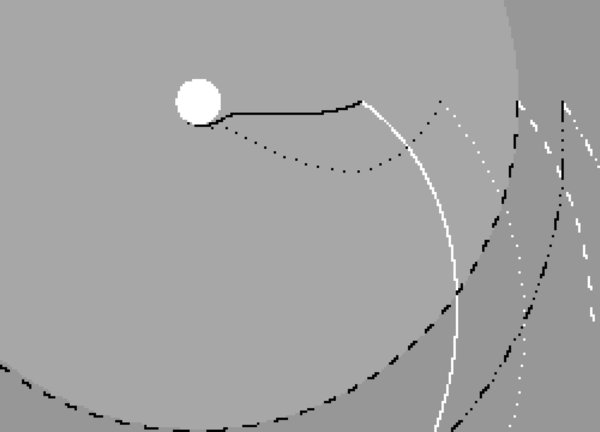
Figure 1. Characteristics  (white lines) and
  (black lines) for the system HD 179949. The light gray circle indicates the Alfvén radius around the star (white disk). The solid lines show the characteristics for the actual planet. The three other linestyles refer to three hypothetical planets on different, more distant orbits: the dashed lines show the characteristics for a hypothetical planet with an orbit at the Alfvén radius, and the dotted lines those for a planet in the middle between this orbit and the actual one. The dash-dotted lines belong to a planet being located outside of the Alfvén radius. The characteristic,
  , can reach the star only if the planet is located within the Alfvén radius of the star, while
  points always away from it.
Download figure:
Standard image High-resolution imageThe phase differences between the hot spot, i.e., the point, where  hits the stellar surface, and the planet are illustrated in Figure 2 for the two planets HD 179949 b (left panel) and υ And b (right panel) according to the model by Preusse et al. (2006). The observed phase difference, Δϕ, is the difference between the angle of the hot spot relative to the starting point, ϕc, and the orbital motion of the planet, ϕp during the travel time of the perturbation (see the figure caption for details). The current model could be shown also to reproduce the observed phase shifts for the HD 189733, τ Boo, as well as that for the more distant planet around the star HD 192263 with a strange phase shift of −90° (Kopp et al. 2009).
Figure 2. Scenario to explain the phase difference Δϕ for HD 1779949 b (60°, left panel) and υ And b (169°, right panel). ϕc is the angle between the starting point of the characteristic,  , and the hot spot, i.e., the point where it hits the stellar surface. ϕp is the angle covered by the planet along its orbit during the travel time t = τc of the perturbation along
  toward the star.
Download figure:
Standard image High-resolution image3. THE INFLUENCE OF A PLANETARY DIPOLE FIELD
Before studying the propagation of magnetic perturbations illustrated above, we first deal with the question of how the planet can generate them. From the system Jupiter–Io we know that Io perturbs the Jovian magnetic field, although it is now generally believed that Io does not possess an intrinsic dipole field (e.g., Saur et al. 2002). Concerning the extrasolar planet, HD 179949 b, Shkolnik et al. (2003) argued that the planet's dipole field should be lower than that of Jupiter because of the planet's slow rotation in consequence of tidal locking, but interpreted their results also toward an indirect detection of a planetary dipole field.
In order to address this point, we performed simulations for HD 179949 b for four different planetary dipole fields as described below. The coordinate system is chosen with the y-axis pointing along the direction of the line star—planet line away from the star, the z-axis is the axis of rotation of the star, pointing from south to north, and the x-axis completes the right-handed system. The origin of this "local" coordinate system is the center of the planet, all lengths are given in units of the planetary radius, where we assumed one Jovian radius (1 RJ = 71,492 km) as the planet's radius.
In this coordinate system, magnetic field and stellar wind velocity have a y-component together with an x-component due to the rotation of the star, the latter also because of the faster orbital motion of the planet (Table 1; Preusse et al. 2006, 2007). Superimposed to this stellar magnetic field is a planetary dipole field with a magnetic moment,  , pointing into positive z-direction. In normalized notation,
  can be given in units of the local value of the stellar wind magnetic field (Bpl,z = −mpl in the equatorial plane, z = 0). Figure 3 shows magnetic field lines in the y–z-plane for the cases mpl = 0 (no intrinsic dipole field, upper left panel), mpl = 1 (lower left panel), mpl = 5 (upper right panel), and mpl = −5 (anti-parallel to the previous case, lower right panel). The figure shows the steady state after the flow around the planet has been initialized (see above), where only some of those field lines are shown that penetrate the planet's surface, in order to illustrate the distortion of the dipole field due to its superposition with the stellar field being shown in the first case (no intrinsic dipole field).
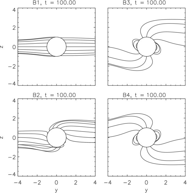
Figure 3. Stationary state of the magnetic field lines in the y–z-plane for different strengths, mpl of the planetary dipole moment: mpl = 0 (B1), 1 (B2), 5 (B3), and −5 (B4), given in normalized units, in the upper left, lower left, upper right, and lower right panels, respectively. Here and in the following figures all length scales are given in planetary radii, and timescales are given in Alfvén times.
Download figure:
Standard image High-resolution imageThe plasma has a small uniform background resistivity, which is enhanced near the planet by a factor of four to model the planetary atmosphere. An optional mass loading term has been set to zero for this case. The result of this interaction is the formation of Alfvén wings (Neubauer 1980), which are connected with an electric current system flowing along the Alfvén characteristics (e.g., Preusse et al. 2006, and references therein). In the present geometry, this current flows above and below the equatorial plane and closes across the planet's conducting atmosphere. A proper quantity to illustrate this current is its component parallel to the magnetic field:
Figure 4 shows this quantity in a plane 1.2 planetary radii above the equatorial plane, i.e., slightly above the planet's surface, for the four cases shown in Figure 1.

Figure 4. Isosurfaces of the parallel component of the electric current density at 1.2 planetary radii above the equatorial plane in normalized units for the four cases of Figure 3. Again, the stationary state is shown.
Download figure:
Standard image High-resolution imageThe first panel, the case with no planetary dipole field, shows the typical arrow-like structure of the Alfvén wings. The three other panels demonstrate how strength and direction of the planetary dipole field modify this structure, in particular it should be noted that the planetary dipole field leads to an increase of the current density. This increase, however, is only visible in the vicinity of the planet, and almost the same current flows in all cases toward the star (y < 0) and away from it (y>0).
Magnetic fields of extrasolar planets can so far only be estimated, e.g., by scaling laws as a function of the rotation period (Sánchez-Lavega 2004; Durand-Manterola 2009), leading to dipole moments between those of Saturn and Jupiter, whereas the model by Christensen et al. (2009) predicts one order of magnitude higher magnetic moments for tidally locked hot Jupiters. At this point, we cannot discuss whether the two planets under consideration, HD 179949 b and υ And b, are magnetized or not. From our simulation results, we can, however, conclude that a current system between planet and star can also be established for an unmagnetized planet. If such a current system already leads to an observable hot spot in the stellar chromosphere—energetic considerations are beyond the scope of the present study—we can conclude that the observation of a magnetic interaction can be interpreted as an indication of a magnetic interaction, but not necessarily for the presence of a planetary dipole field.
4. MAGNETIC INTERACTION BETWEEN PLANET AND STAR
In this section we perform global simulations of the interaction for both planets in order to check our theoretical model (Preusse et al. 2006), which is briefly sketched above. As a result of the previous section, we omit a planetary dipole field and merely enhance the resistivity near the planet.
Figures 5 and 6 show the results of the global, cylindrical simulations transformed to a Cartesian coordinate system for the stars HD 179949 and υ And, respectively. In this "global" coordinate system the main direction of the stellar wind at the initial position of the planet is the x-axis, in contrast to the local system used above. Again, all length scales are given in planetary radii, where we assumed one Jovian radius also for υ And. The radius of the planet merely affects the normalization, in particular the timescale. For numerical reasons, in particular the strong gradient of the gravitational field the inner boundary of the computational area had to be limited to two stellar radii.
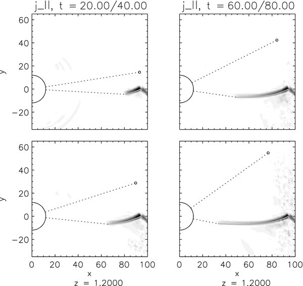
Figure 5. Temporal evolution of a magnetic perturbation in the system HD 179949, generated by the planet at t = 0 on the x-axis. The time is given normalized to the Alfvén travel time; four snapshots are shown: t = τ1 = 20 (upper left panel), τ2 = 40 (lower left), τ3 = 60 (upper right), and τ4 = 80 (lower right); distances are given in planetary radii. The gray scale codes |j∥| at 1.2 planetary radii above the equatorial plane. The small circle and the dotted line indicate the planet (to scale) and the radius vector to the planet at the given times, respectively. The thick black line shows that part,  , of the Alfvén characteristic, which has been covered by the perturbation up to the respective snapshot time. The second dotted line connects its end point with the center of the star (large circle at the origin). The angle between the two dotted lines (counted counterclockwise from the upper line to the lower one) shows, thus, the "evolution" of the phase angle, i.e., the gray area in Figure 2.
Download figure:
Standard image High-resolution image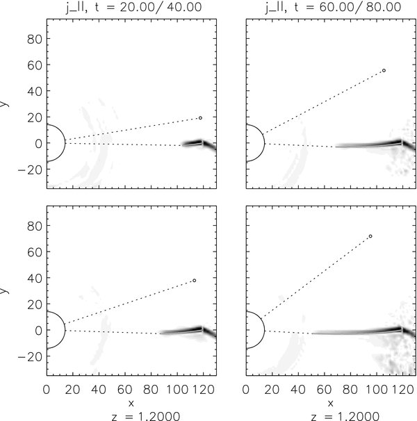
Figure 6. Same as Figure 5, but for the system υ And. Besides the main current system, here and in Figure 5 some regions with small perturbations evolve, probably due to limited grid resolution (affecting mainly the gravitational term) and the background resistivity.
Download figure:
Standard image High-resolution image
At time t = 0, the planet is located, as mentioned above, on the x-axis and triggers a perturbation of the stellar magnetic field. This perturbation generates an electric current system resembling that between Jupiter and Io. Due to the different geometry of the extrasolar planetary systems, however, this current flows above and below the equatorial plane and closes across the planet's ionosphere. As an indicator for this current system and its propagation, the parallel current density, defined in Equation (3), is plotted. The time is given in Alfvén travel times, τA. The four panels of both figures show snapshots, τi, i = 1...4, of the system at 20, 40, 60, and 80 τA. The Alfvén times are 331 s (5 minutes 31 s) for HD 179949 b and 232 s (3 minutes 52 s) for υ And b. Superimposed to this plot are the star (large semi-circle at the center of the coordinate system) and the planet (small circle) at its positions to the respective times, τi, the dotted line helps to read the covered angle, ϕp(t). The second superimposed quantity is the Alfvén characteristic,  , integrated with the initial solution for the stellar wind until t = τi. The dotted line connects the end point of
  with the stellar center and indicates the angle, ϕc(t). The radii of star and planet are plotted to scale, the parallel current density is given in normalized values.
The phase difference, Δϕ(t) = ϕc(t) − ϕp(t), is the angle between the upper and lower dotted lines, respectively, measured counterclockwise. The observed phase difference is Δϕ(τc), where τc is the time, at which the characteristic hits the stellar surface. The characteristic from HD 179949 b reaches the star after 424 τA, that from υ And b after 578 τA, corresponding to 1.62 and 1.55 days, respectively.
The figures depict how the electric current system propagates along the Alfvén characteristics shown analytically in Figure 2. While the characteristic, c(+)A, is directed away from the star, c(−)A finally hits the stellar surface. As an indicator for the positions of the perturbation at the respective snapshots, τi ∈ {20, 40, 60, 80}, and, thus for its propagation velocity, we can use the front of the current system, i.e., j∥ is different from zero up to the point where  ends. The entire course of the perturbation up to the various snapshots can be investigated by comparing the isosurfaces of j∥ with the characteristic,
  . For both planetary systems, we observe a remarkable coincidence between numerical simulations and theoretical prediction at all four snapshots, so that the numerical simulations confirm the analytical theory.
A closer inspection of the simulation results reveals that  accelerates, in agreement with the semi-analytical solution for the initial configuration, until about 60 τA (≈53τA for HD 179949 b, ≈58τA for υ And b) and afterward becomes slower and slower. For the case of our simulations, however, the inner boundary of the computational area had to be set to two stellar radii, which is already reached after 105τA and 125τA for HD 179949 b and υ And b, respectively, so that we could follow only just under one quarter of the entire process. Nevertheless, we may state that our simulations confirm the theory by Preusse et al. (2006) not only qualitatively, but also quantitatively, and hope that improved numerical models will also enable us to verify the model closer to the star and, thus, the predicted phase shift.
5. SUMMARY AND DISCUSSION
In this paper, we showed results from MHD simulations of the magnetic interaction of close-in extrasolar planets with their host stars. Starting from the observations by Shkolnik et al. (2003) and Shkolnik et al. (2005) of so-called hot spots in the chromospheres of the stars HD 179949 and υ And, respectively, we addressed two major questions: can these observations be interpreted as toward the discovery of a planetary magnetic field of the planets HD 179949 b and υ And b? Can the analytical model by Preusse et al. (2006) to explain the observed phase angles between the hot spot and the substellar point (i.e., the inferior conjunction of the planet) be confirmed by numerical simulations?
The model by Preusse et al. (2006) deals with the perturbation of the stellar magnetic field by the planet and the propagation of such perturbations in the stellar wind on more global scales, where no structure of the coronal magnetic field inside the source surface is taken into account. The models by McIvor et al. (2006), Lanza (2008, 2009), and Cohen et al. (2009), in contrast, mainly concern the "local" structure of the coronal field close to the star. These two different approaches are certainly not mutually exclusive, and it appears not unlikely that a combination of the "global" model by Preusse et al. (2006) with one or more of the "local" models will provide even more realistic results. As a first step toward such a "hybrid" approach, we reinvestigated our analytical model numerically and also studied the influence of a planetary dipole field as mentioned above.
The detailed results can be summarized as follows: although it appears very reasonable that hot Jupiters are magnetized, the simulations demonstrate that a field-aligned current system develops even in the absence of a planetary dipole field. Differences between the unmagnetized and the magnetized case are visible merely within several planetary radii. If such a current system leads to an observable hot spot, one cannot conclude that the detection of a magnetic interaction between planet and star can also be necessarily interpreted as the detection of a planetary magnetic field. It should be noted, however, that our investigations did so far not take into account any energetic considerations. A possible scenario for the generation of the hot spot could be particle acceleration in a resistive region in the stellar chromosphere by magnetic reconnection similar to that suggested by Kopp et al. (1998) for the interaction between Io and Jupiter. Such questions are, however, beyond the scope of the present study.
In order to investigate the model by Preusse et al. (2006) by numerical simulations, we performed global simulations of the interaction between planet and star with an unmagnetized planet and took the electric current density, j∥, along the magnetic field as an indicator. Due to technical limitations of the present numerical model, the inner boundary had to be limited to two stellar radii, so that the current system closer to the star could not be followed. For the part between the star and this boundary, however, we obtained for both planets a qualitatively and quantitatively excellent agreement between theoretical prediction and numerical simulations, so that we may consider our numerical simulations as a strong confirmation of our analytical theory. We hope to be able to simulate the part closer to the star with a future version of the numerical model.
We thank Horst Fichtner for helpful comments and his critical reading of the manuscript and also the two anonymous referees, whose contributions helped to significantly improve our paper. The work by A.K. benefitted from financial support through the Research Unit FOR 1048 (project FI 706/8-1) funded by the Deutsche Forschungsgemeinschaft.
Footnotes
- 4