


ABSTRACT
Type III radio bursts are produced near the local electron plasma frequency fp and near its harmonic 2fp by fast electrons ejected from the solar active regions and moving through the corona and solar wind. The coronal bursts have dynamic spectra with frequency rapidly falling with time, the typical duration being about 1–3 s. In the present paper, 37 well-defined coronal type III radio bursts (25–450 MHz) are analyzed. The results obtained substantiate an earlier statement that the dependence of the central frequency of the emission on time can be fitted to a power-law model, f(t) ∝ (t − t0)−α, where α can be as low as 1. In the case of negligible plasma acceleration and conical flow, it means that the electron number density within about 1 solar radius above the photosphere will decrease as r−2, like in the solar wind. For the data set chosen, the index α varies in the range from 0.2 to 7 or bigger, with mean and median values of 1.2 and 0.5, respectively. A surprisingly large fraction of events, 84%, have α ⩽ 1.2. These results provide strong evidence that in the type III source regions the electron number density scales as n(r) ∝ (r − r0)−β, with minimum, mean, and median β = 2α of 0.4, 2.4, and 1.0, respectively. Hence, the typical density profiles are more gently sloping than those given by existing empirical coronal models. Several events are found with a wind-like dependence of burst frequency on time. Smaller power-law indices could result from the effects of non-conical geometry of the plasma flow tubes, deceleration of coronal plasma, and/or the curvature of the magnetic field lines. The last effect is shown to be too weak to explain such low power-law indices. A strong tendency is found for bursts from the same group to have similar power-law indices, thereby favoring the hypothesis that they are usually produced by the same source region.
Export citation and abstract BibTeX RIS
1. INTRODUCTION
The solar corona structure is still a hot topic of solar physics. Early observations and theories suggested that it is relatively simple and consists of several spherical layers, while later it was recognized that the corona is complicated and intrinsically time-dependent (e.g., Schrijver et al. 1997, 1998; Aschwanden et al. 2001; Schrijver 2005; Zurbuchen 2007). Nevertheless, simple empirical models of coronal plasma density are still widely used in solar physics and space weather studies. For instance, for the quiet corona Newkirk (1961) suggested a hydrostatic equilibrium model, which is exponential, nN(r) = 4.2 × 10⁴exp(4.32 r−1). Other models involve finite sums of power-law terms with different indices: the Baumbach–Allen model nBA(r) = 108(1.55 r−6 + 2.99 r−16) (Baumbach 1937; Allen 1947), the Saito model nS(r) = 1.36 × 10⁶ r−2.14 + 1.68 × 10⁸ r−6.13 (Saito et al. 1977), and the radio-derived model of Leblanc et al. (1998), nL(r) = 3.3 × 10⁵ r−2 + 4.1 × 10⁶ r−4 + 8.0 × 10⁷ r−6. All the electron number densities n are measured in cm−3 and distances r in units of the solar radius r☉. The high index terms dominate at sufficiently small r, while the r−2 terms describe conservation of number of electrons for a spherically symmetric, constant speed, outflow like the solar wind (Parker 1958). Mann et al.'s (1999) model is a fit to data of special solutions to Parker's wind equation. It is Newkirk-like for r < 1.3 r☉ and n(r) ∝ r−2.16 for r>0.2 AU. An empirical model of Robinson & Cairns (1998) with nRC(r) ∝ (r − r☉)−2.19, while unique in having an offset r☉, is based on fitting interplanetary radio data for r ≫ r☉. Recently, Cairns et al. (2009) have interpreted the high indices of terms like r−6 and r−16 as artifact of placing the corona's mathematical origin at r = 0 rather than at non-zero distance of order of the solar radius.
Because of their relatively simple underlying physics, type III radio bursts are considered to be a valuable tool for radio probing of the corona and solar wind (e.g., Bhonsle et al. 1979; Warmuth & Mann 2005). These bursts are associated with streams of relativistic electrons moving away from the Sun with approximately constant speed along open magnetic field lines. The type III radio emission is produced near the local plasma frequency fp or its harmonic 2fp. Since fp(r) = 9 n1/2 kHz for n in cm−3, this emission provides direct information about local plasma density in the source region. Observations of type III bursts were used to develop solar wind and coronal density models (Alvarez & Haddock 1973; Leblanc et al. 1998).
It is generally accepted that in the low solar corona (r ≲ 2 r☉), where the meter-wavelength type II and III bursts originate, the plasma density profile shows a steep falloff, which can be described by terms with power-law indices −6 or −16. However, examination of type II bursts showed that the absolute values of the observed indices are considerably smaller, 1.2–2.6 (Lobzin et al. 2008), and can be as low as those in the solar wind. If the speed of the emission source is assumed to be approximately constant, the observed relatively small absolute values of the power-law indices can be considered as appropriate estimates of the power-law indices for the electron number density profiles, thereby implying that wind-like regions may exist deep in the corona (Lobzin et al. 2008). With type II bursts, which are associated with shock waves, an alternative explanation exists, i.e., the speed of the shock wave may vary in such a way that the observed value of the index, which is derived from the dependence of the observed frequency on time, differs considerably from values which could be derived from direct density measurements (Lobzin et al. 2008). Because it is impossible to study shock dynamics in highly inhomogeneous solar plasma without additional information, it is rather difficult to discriminate between these two interpretations. However, recent studies of several coronal type III bursts have provided direct evidence that wind-like regions do exist deep in the corona (Cairns et al. 2009). Cairns et al. (2009) also suggested an interpretation of these observations in terms of conical flows originating not far from the solar surface, i.e., instead of a spherically symmetric radial flow there is a localized outflow confined to a cone whose apex is near the photosphere.
The main purpose of this paper is to extend the Cairns et al. (2009) analysis and estimate the plasma density power-law indices β from a significant sample of coronal type III bursts. For the present study, the data processing method used by Cairns et al. (2009) has been modified. The modified technique is more robust and allows one to obtain more quantitative estimates for the same data set. This paper presents results of the analysis of 37 type III bursts. This data set is large enough to make a statistical inference about occurrence rates for different power-law indices. It is confirmed that the wind-like values of β reported by Cairns et al. (2009) are quite typical, as are even lower values. The paper is organized as follows. The data used in the study are described in Section 2. The procedures for data processing and analysis of type III radio bursts are presented in Section 3. The results obtained are outlined in Section 4 and discussed in Section 5. Section 6 gives conclusions.
2. OBSERVATIONS
This study uses radio observations obtained from two different radiospectrographs. The first instrument, Potsdam-Tremsdorf Radiospectrograph, is located near the village of Tremsdorf 15 km south-east of Potsdam (52 28 N, 1313 E). The instrument consists of four sweep spectrographs covering the frequency range 40–800 MHz with a time resolution of 0.1 s. The set of spectrographs is fed by a system of four different aerials in the bands 40–100 MHz, 100–170 MHz, 200–400 MHz, and 400–800 MHz (Mann et al. 1992). There is a gap between the second and third bands because of very strong interference due to local UHF TV. Other strong artificial interference in the frequency range of interest is in the ranges 85–108 MHz and 550–700 MHz due to local UHF radio and VHF TV, respectively. Further details can be found in the paper by Mann et al. (1992).
The second instrument, IZMIRAN's spectrograph, is located in the Moscow region (5547 N, 3732 E). It consists of four receivers scanning the frequency ranges 25–50 MHz, 45–90 MHz, 90–180 MHz, and 180–270 MHz. The time resolution is 0.04 s in patrol mode. Further details can be found in the paper by Gorgutsa et al. (2001).
From the available data, 37 type III events (some single bursts and others from groups) were selected. The selection criteria were as follows.
- 1.A type III burst is clearly visible for frequencies below ∼450 MHz.
- 2.The burst contains at least one part that is contiguous with respect to time and frequency, i.e., there are no wide gaps due to missing and/or bad measurements, and the contiguous part that is not strongly affected by interference occupies a frequency range of 0.59 octaves or more, i.e., fmax /fmin ≳ 1.5, where fmax and fmin are the maximum and minimum frequencies of the contiguous part, respectively. Narrow-band interference is unavoidable and is allowed to cross the chosen part of the type III burst.
- 3.The burst is well separated from its type III neighbors and other wide-band emissions that may precede or follow it, meaning negligible overlap in frequency-time space.
- 4.For almost all frequencies, the duration of the signal is considerably shorter than the time interval between the two intensity maxima observed at the highest and lowest frequencies for the contiguous part.
- 5.There is no evidence of harmonic structure for the burst.
When all these criteria are satisfied, the burst contains a contiguous part in which only fundamental or harmonic emission is observed and the frequency drift is easily seen and can be quantitatively estimated. At higher frequencies, the drift is usually too fast to be evaluated with the given time resolution of the spectrographs. The list of the events chosen is shown in Table 1.
Table 1. The Results of Power-law Fitting for Type III Radio Bursts
| Event | Group | Date | Start | End | Minimum | Maximum | Ratio | Power-law Indices for fp | ||
|---|---|---|---|---|---|---|---|---|---|---|
| Number | Number | Times | Times | Frequencyc | Frequencyc |  |
Best | Min | Max | |
| (UT) | (UT) | fmin (MHz) | fmax (MHz) | |||||||
| 1a | I | 19970402 | 05:45:50 | 05:45:51 | 110 | 400 | 3.6 | 1 | 0.7 | 1.5 |
| 2a | I | 19970402 | 05:45:52 | 05:45:53 | 112 | 450 | 4.0 | 0.9 | 0.7 | 1.7 |
| 3a | I | 19970402 | 05:45:55 | 05:45:57 | 112 | 450 | 4.0 | 1.2 | 0.6 | 1.7 |
| 4a | 19980508 | 05:58:53 | 05:58:55 | 47 | 84 | 1.8 | 7.0 | 1.0 | 7.0 | |
| 5a | II | 19980607 | 09:18:07 | 09:18:13 | 42 | 85 | 2.0 | 1.8 | 1.2 | 3.3 |
| 6a | II | 19980607 | 09:18:45 | 09:18:47 | 42 | 85 | 2.0 | 1.2 | 0.8 | 3.2 |
| 7a | 19980731 | 05:39:18 | 05:39:23 | 40 | 85 | 2.1 | 0.8 | 0.7 | 1.2 | |
| 8a | 19980819 | 14:09:30 | 14:09:33 | 49 | 128 | 2.6 | 0.5 | 0.5 | 0.5 | |
| 9a | 19980831 | 15:34:34 | 15:34:36 | 109 | 170 | 1.6 | 0.4 | 0.3 | 0.5 | |
| 10a | III | 19990221 | 09:41:39 | 09:41:43 | 111 | 170 | 1.5 | 0.3 | 0.3 | 0.3 |
| 11a | III | 19990221 | 09:42:26 | 09:42:28 | 111 | 170 | 1.5 | 0.4 | 0.3 | 0.6 |
| 12a | III | 19990221 | 09:42:47 | 09:42:48 | 111 | 170 | 1.5 | 0.6 | 0.5 | 0.8 |
| 13a | III | 19990221 | 09:45:00 | 09:45:01 | 111 | 170 | 1.5 | 0.6 | 0.4 | 1.2 |
| 14a | III | 19990221 | 09:45:15 | 09:45:17 | 111 | 170 | 1.5 | 0.5 | 0.5 | 0.6 |
| 15a | IV | 19991020 | 09:25:51 | 09:26:02 | 40 | 170 | 4.3 | 1.0 | 1.0 | 1.0 |
| 16a | IV | 19991020 | 09:26:17 | 09:26:23 | 40 | 82 | 2.1 | 0.8 | 0.7 | 1.3 |
| 17a | 20000228 | 10:51:39 | 10:51:41 | 45 | 82 | 1.8 | 0.3 | 0.2 | 0.4 | |
| 18a | V | 20000418 | 11:46:19 | 11:46:25 | 40 | 85 | 2.1 | 7.0 | 4.0 | 7.0 |
| 19a | V | 20000418 | 11:53:24 | 11:53:31 | 42 | 78 | 1.8 | 0.2 | 0.2 | 0.2 |
| 20a | 20010328 | 08:46:42 | 08:46:47 | 40 | 170 | 4.3 | 0.8 | 0.7 | 0.9 | |
| 21b | VI | 20010412 | 10:18:07 | 10:18:10 | 25 | 49 | 1.9 | 0.3 | 0.2 | 0.7 |
| 22b | VI | 20010412 | 10:19:07 | 10:19:11 | 32 | 60 | 1.9 | 0.4 | 0.3 | 0.6 |
| 23a | 20010831 | 10:34:07 | 10:34:13 | 42 | 83 | 2.0 | 0.6 | 0.5 | 0.8 | |
| 24b | 20010917 | 08:21:06 | 08:21:08 | 25 | 45 | 1.8 | 0.6 | 0.4 | 0.7 | |
| 25b | 20010928 | 08:12:09 | 08:12:17 | 25 | 90 | 3.6 | 0.5 | 0.4 | 0.7 | |
| 26a | VII | 20011022 | 14:46:52 | 14:46:58 | 42 | 78 | 1.8 | 0.3 | 0.2 | 0.3 |
| 27a | VII | 20011022 | 14:51:19 | 14:51:21 | 109 | 170 | 1.6 | 0.2 | 0.2 | 0.3 |
| 28b | 20011229 | 09:39:46 | 09:39:50 | 30 | 45 | 1.5 | 0.2 | 0.2 | 0.4 | |
| 29b | VIII | 20030717 | 08:18:37 | 08:18:39 | 114 | 197 | 1.7 | 0.3 | 0.2 | 0.4 |
| 30b | VIII | 20030717 | 08:19:30 | 08:19:35 | 31 | 45 | 1.5 | 0.2 | 0.2 | 0.2 |
| 31b | 20030819 | 07:55:13 | 07:55:16 | 116 | 197 | 1.7 | 0.4 | 0.3 | 0.7 | |
| 32b | 20031103 | 09:49:32 | 09:49:36 | 28 | 44 | 1.6 | 0.4 | 0.3 | 0.8 | |
| 33a | IX | 20031118 | 08:35:18 | 08:35:22 | 40 | 83 | 2.1 | 7.0 | 2.5 | 7.0 |
| 34a | IX | 20031118 | 08:35:35 | 08:35:38 | 40 | 83 | 2.1 | 2.8 | 1.5 | 7.0 |
| 35a | IX | 20031118 | 08:36:48 | 08:36:53 | 40 | 83 | 2.1 | 2.3 | 1.1 | 6.9 |
| 36a | IX | 20031118 | 08:36:57 | 08:37:03 | 40 | 83 | 2.1 | 0.5 | 0.4 | 0.6 |
| 37b | 20060430 | 09:26:12 | 09:26:14 | 31 | 45 | 1.5 | 0.2 | 0.2 | 0.2 | |
Notes. aData of Potsdam-Tremsdorf Radiospectrograph. bData of IZMIRAN Radiospectrograph. cThese frequencies are related to the processed spectra rather than to the type III bursts, which typically occupy a wider frequency range.
Download table as: ASCIITypeset image
3. DATA ANALYSIS
The data processing procedure is illustrated using a type III burst observed by the Potsdam spectrograph on 1999 October 20 at 09:26 UT (event 15 in Table 1). Figure 1(a) shows the dynamic spectrum. The burst satisfies all the criteria mentioned in the previous section. Although it is split by narrow-band interference, which is particularly strong in a rather wide range 85–108 MHz, there is an evident correspondence between the high- and low-frequency parts of the burst. It is also far apart from its neighbors. This allows one to combine the high- and low-frequency parts and process them together. The entire burst is clearly visible in the frequency range 40–170 MHz, occupying more than 2 octaves.
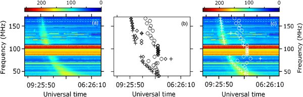
Figure 1. Illustration of the method for data processing. (a) Frequency-time dynamic spectrum of the type III burst of 09:26 UT on 1999 October 20 (event 15). The colorbars (grayscales in the print version) show the levels of normalized intensities. (b) Frequency-time dependences obtained with different power-law indices in Equation (1): circles, diamonds, and plus symbols correspond to γ = 1, 5, and 100, respectively. (c) Spectrum with the frequency-time dependences obtained with γ = 1 (circles) and 100 (plus symbols) superposed.
Download figure:
Standard image High-resolution imageLet I(it, if) be an array of intensities for a chosen portion of the dynamic spectrum, the first and second indices corresponding to time and frequency, respectively. To describe the shape of a type III burst quantitatively (i.e., to determine the best function describing its frequency drift), for each frequency f(if) within the range chosen we find the time t(itc) corresponding to the "center" of the intensity hump for the burst under consideration. The time index for the center of the hump is defined as follows:
where γ is a power-law index. Obviously, this definition is similar to that of the center of mass of the set of particles, with the analog of mass being proportional to Iγ.
Previously, the times corresponding to the maximum signal strength were used rather than itc (Cairns et al. 2009). However, the current approach is found to be more robust and allows us to process more events quantitatively. The best value of γ is found empirically. It is easily seen that the contribution of high intensities increases with an increase in γ. Figure 1(b) shows the series of points (ti, fi) obtained for several different values of γ, including a relatively small value of 1 and an optimum value of 100. It is easily seen that as the γ increases, most of the points approach the points corresponding to the biggest values of γ and their scatter decreases. Figure 1(c) reproduces the type III spectrum with two series overlaid, those for γ = 1 and 100. It shows that most of the points for γ = 100 are in a vicinity of the burst's crest, confirming that this value of power-law index is nearly optimal, while the lowest value is definitely not.
In addition, we observe that the positions of the points corresponding to intense narrow-band interference do not change significantly as γ changes. Rather, the points are concentrated in the middle of the processed part of the spectrum, as should be expected from Equation (1) provided that the interference intensity does not vary considerably with time. If the burst under consideration is well separated from others, it is possible to choose a portion of spectrum such that the outliers related to such interference are far apart from the burst. Hence, they are easy to separate and reject. This feature increases the robustness of the method and allows one to find better fits and improve the accuracy of their parameters.
Even without outliers, the points (ti, fi) usually do not lie on a smooth curve. Rather, they show considerable fluctuations which can be attributed to measurement errors. The next stage of data processing is the fitting of the model function f = f(t; p), depending on adjustable parameters p, to the set of measured pairs (ti, fi). The derivation of the expression for a suitable model function is described in detail by Lobzin et al. (2008) and Cairns et al. (2009) and reproduced here for self-sufficiency. Suppose that the source of the emission starts from a position r0 at time t0 and moves with a constant speed v, then r(t) = r0 + v(t − t0). Because type III bursts are known to be produced by beams of energetic electrons moving along a magnetic field line, r is the distance measured along this field line. The emission frequency is close to the local plasma frequency, fp and/or its harmonic, 2fp. Thus, in the inhomogeneous solar corona the frequency of the emission varies with time. For most cases, it decreases because the electrons move away from the Sun into its corona with decreasing plasma density. If we assume further that in the region of interest, the plasma frequency obeys a power law along the magnetic field line, i.e., fp ∝ (r − r1)−α, where r1 and α are constants, then the model function can be chosen in the form:

where a and b are constants. Because  , where n is the electron number density, the power-law index for the local plasma density is β = 2α. Thus, by fitting the model (Equation (2)) to the observed time-varying radiation frequency, the index β can be obtained independent of v or the absolute scale of r. The same model was previously used by Cairns et al. (2009) to analyze a few type III bursts, extending the earlier model of Lobzin et al. (2008) for type II solar radio bursts.
In the calculations related to processing of type III radio bursts, which have short durations, it is more convenient to replace the model function f = f(t) by the inverse function t = t(f). For each particular event, we find the maximum and minimum frequencies, f0 and f1, respectively. If it is assumed that the emission starts at t0 with frequency f0 and is then observed up to t = t1 when its frequency equals f1, the model function t = t(f; t0, t1, f0, f1, α) corresponding to Equation (2) is given by
Since the deviations from the model are unlikely to be normally distributed and obviously result in outliers, least-squares fitting is inappropriate (see, e.g., Press et al. 1997). Instead, we use a robust technique of minimizing the sum of absolute deviations:
The merit function X depends on adjustable parameters t0, t1, f0, f1, and α. The best value of the power-law index α is found by minimizing X over all five parameters.
The results of fitting are summarized in Table 1. In addition to the best values of the power-law indices, also shown are their minimum and maximum values corresponding approximately to the 68% confidence interval. Note that in general the best value does not coincide with the middle of the interval between the minimum and maximum values, because the merit function X is not symmetric with respect to its minimum at the best value of α. Rather, it increases more quickly as α decreases rather than in the opposite direction. This makes large power-law indices more difficult to estimate than small ones. As α increases, the power-law fit given by Equation (3) becomes very close to the exponential:
Accordingly, if the frequency range is narrow and the scatter of data points is large, it can be impossible to distinguish a power-law dependence with large index from the exponential. In the present paper, we consider values of α ⩾ 7 as infinitely large numbers corresponding to the exponential law. It is worth mentioning that the coronal plasma density models suggested by Allen (1947), Baumbach (1937), and Leblanc et al. (1998) contain terms proportional to r−16 and r−6, so for small heights above the photosphere the local plasma frequency is expected to scale as r−α with 3 ⩽ α ⩽ 8, while Newkirk (1961) presented an exponential model.
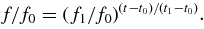
The results obtained for event 15 are presented in Figures 1 and 2(a)–(c); these show dynamic spectra in coordinates f versus t and 1/f versus t and plots for the data points corresponding to the frequency-dependent centers of the burst and the best power-law fit. The best value of the power-law index is found to be surprisingly low, α = 1.0, the value expected for the solar wind rather than the deep corona, as discussed in Section 1. For comparison, the exponential dependence and the power-law curve with index α = 3 are also shown. Visual inspection of the plots confirms that the fit with α = 1.0 is the best one, while the exponential and the power-law dependence with α = 3 are definitely too steep and are not appropriate for this event.
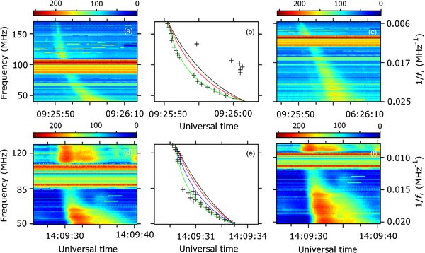
Figure 2. Dynamic spectra of type III radio bursts occupying more than 1 octave in frequency and power-law fits. The colorbars (grayscales in the print version) show the levels of normalized intensities. The bursts were observed on (a) 1999 October 20 (event 15) and (d) 1998 August 19 (event 8). (c and f) The same spectra upon 1/f transformation. (b and e) The green line (solid line in the print version) shows the best power-law fits to the data points. Also shown for comparison are the power-law dependences with α = 1 and 3 (blue and red lines, respectively; in the print version, dashed and dot-dashed lines, respectively) and the exponential dependence (black line, dotted in print). For event 15, the green (solid) and blue (dashed) lines coincide. The vertical axes for the middle panels correspond to frequency.
Download figure:
Standard image High-resolution imageFigure 2(b) illustrates the fact that reliable estimates of power-law indices α can be obtained if the scatter of data points is not too large. A distinction between two different power-law dependences or between a power law and the exponential can be made provided that the data scatter along the time axis is smaller than the maximum distance between the curves in this direction. Obviously, more reliable and precise estimates require a wider frequency range in which the frequency drift is measurable.
For several reasons related to the selection criteria in Section 2, including strong interference and event overlap, for most events studied the frequency range analyzed is only about 1 octave. Rather often this will not allow precise estimation of the power-law index α, especially if it seems to be large, but sometimes it is still possible to make a distinction between the best fit and solar-wind-like dependence with α = 1. Examples of such events will be provided in the next section.
4. RESULTS
For brevity, the power-law indices will be referred to as wind-like if α ⩽ 1.2, since these correspond to density indices β = 2α ⩽ 2.4. The reason for this definition is that the plasma density in the distant solar wind is known to decrease with distance as n ∝ r−2, and the corresponding power-law index for plasma frequency is 1. In contrast, old models for the lower corona (e.g., Baumbach 1937; Allen 1947; Leblanc et al. 1998) have the density scaling as r−6, r−16, thereby resulting in power-law indices for plasma frequency in the range from 3 to 8.
Figure 2 shows two well-defined, well-separated, coronal type III bursts (events 15 and 8 in Table 1) with a large frequency extent. These events were observed on 1999 October 20 and 1998 August 19, respectively. Panels (b) and (e) show the corresponding sets of pairs (t, f) and the best fits. Also shown are the curves for power-law indices α = 1 and 3, as well as exponential dependences, all of them are constrained to pass through the end points of the best-fit line. For event 15, the best power-law index is equal to 1 with an accuracy better than 0.1, in good agreement with the previous result α = 1.00 ± 0.15 (Cairns et al. 2009), while fits with α = 3 and exponential behavior are strongly contraindicated. For event 8, the best power-law index is even smaller, α = 0.5.
If α ≈ 1, the burst spectrum plotted in coordinates 1/f versus t should give approximately straight lanes, as is easily seen in Figure 2(c). Deviations of the power-law index value from 1 will result in curvature of the emission band. In particular, for α < 1 the band will be deflected to lower values of 1/f, as seen in Figure 2(f).
Bursts like those shown in Figure 2 are rather exceptional. Usually, the contiguous low-frequency parts of bursts occupy less than 1 octave. Figure 3 shows two quite typical type III bursts with such smaller frequency extent. These bursts were observed on 2000 April 18 (event 19) and 2001 December 29 (event 28). The scatter of the data points is not large and allows us to conclude that the best power-law indices for these two events are as low as 0.2. Hence, these bursts are wind-like and the curvature of their bands upon 1/f transformation confirms this conclusion (see Figures 3(c) and (f)).
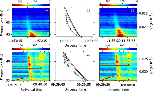
Figure 3. Dynamic spectra of type III radio bursts occupying less than 1 octave in frequency. The colorbars (grayscales in the print version) show the levels of normalized intensities. The bursts were observed on (a) 2000 April 18 (event 19) and (d) 2001 December 29 (event 28). (c and f) The same spectra upon 1/f transformation. (b and e) The green line (solid line in the print version) shows the best power-law fits to the data points. Also shown for comparison are the power-law dependences with α = 1 and 3 (blue and red lines, respectively; in the print version, dashed and dot-dashed lines, respectively) and the exponential dependence (black line, dotted in print). The vertical axes for the middle panels correspond to frequency.
Download figure:
Standard image High-resolution imageThe results of processing of the entire data set are summarized in Table 1, which shows the best power-law indices and their minimum and maximum values corresponding to the boundaries of the 68% confidence intervals. The histogram of the best power-law indices is shown in Figure 4. Surprisingly, most events (31 out of 37 or 84%) have a wind-like index (0.8 ⩽ α ⩽ 1.2) or even smaller, down to 0.2–0.3, with mean and median values of 1.2 and 0.5, respectively.
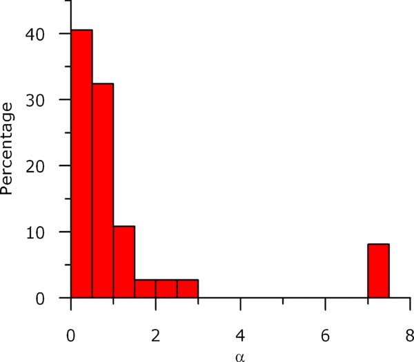
Figure 4. Histogram for the best power-law indices found for events shown in Table 1.
Download figure:
Standard image High-resolution imageWhen estimating occurrence probabilities for different kinds of density profiles, it is necessary to take into account that there exist nine groups of bursts in Table 1. Most likely bursts from the same group are produced by the same source region (it is worth noting that the bursts that appear to be single upon inspection of Table 1 are not necessarily single in the observed dynamic spectra but may belong to a group; however, in these cases the power-law indices can be estimated only for one or a few bursts in each group and only these bursts are mentioned in Table 1). Typically, the bursts from a given group do have similar power-law indices. To estimate a probability for density profiles to be wind-like or steeper, it is thus necessary to take only one burst from each group as a representative of a given source region. If bursts are attributed to the same group because they are close to each other in time but their power-law indices are significantly different, we may argue that the bursts are probably produced by different regions and take them into account separately. Six groups (I, III, IV, VI, VII, and VIII) combine bursts with similar indices, which are wind-like or smaller. These groups provide six wind-like bursts altogether. Other three groups (II, V, and VII) provide one wind-like and one "high-index" bursts each, which we consider as single. In addition, there are 12 single wind-like bursts and 1 single "high-index" burst. Thus, the total number of independent wind-like and "high-index" events are 6 + 3 + 12 = 21 and 3 + 1 = 4, respectively, and the probability of wind-like conditions to occur can be estimated as 21/(21 + 4) = 84%, in agreement with the estimate above, while steeper profiles, which were expected to be more typical for solar corona, are observed only in 16% cases.
For many events like those shown in Figure 5, a relatively small frequency range for the contiguous part of the bursts, insufficient time resolution at high frequencies, and/or confusion between fundamental and harmonic bands or with other events, prevent accurate determination of the power law index α. However, in many cases deviations from straight lines in 1/f versus t plots are still clearly visible and allow one to determine whether α < 1 or α>1. Figure 5 shows two groups of type III bursts with different power-law indices α. The first group, which is referred to as a group VI in Table 1, was observed on 2001 April 12 and has α < 1 (see Figures 5(a) and (b)). Indeed, it is clearly seen that the emission bands deviate from a straight line to smaller values of 1/f as 1/f increases. The curvature of the emission band has an opposite sign for the bursts observed on 2004 April 27 (see Figures 5(c) and (d)), so α>1. It is worth noting that the bursts in each group seem to have similar profiles, in agreement with most results shown in Table 1. Although it is difficult to estimate the power-law indices quantitatively for each burst in such groups, because of overlapping of the bursts and other unfavorable factors, it is still possible to observe the curvature of their bands in 1/f versus t coordinates. Other examples of such groups were shown in Figure 2 in the paper by Cairns et al. (2009). Thus, we may argue that groups of type III bursts usually originate from a localized region in the corona, where the plasma density profile and geometry of magnetic field do not vary significantly.
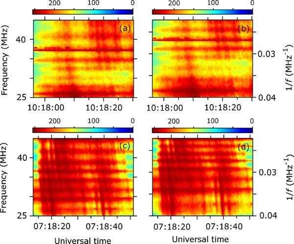
Figure 5. f vs. t and 1/f vs. t dynamic spectra of multiple type III bursts with different power-law indices α. The colorbars (grayscales in the print version) show the levels of normalized intensities. (a and b) Group of bursts observed on 2001 April 12 (group VI in Table 1) with α < 1. (c and d) Bursts observed on 2004 April 27 with α>1.
Download figure:
Standard image High-resolution image5. DISCUSSION
Radio burst frequencies are indicative of the distances between their sources and the Sun (e.g., McLean 1985; Warmuth & Mann 2005). From the Baumbach–Allen density model (Baumbach 1937; Allen 1947), it follows that the frequencies of 150 and 20 MHz correspond to heliocentric distances of 1.04 r☉ and 1.8 r☉, respectively. Several density models (e.g., Baumbach 1937; Allen 1947; Leblanc et al. 1998) suggest that for such range of heliocentric distances the density and plasma frequency scale as n ∝ r−2α and fp ∝ r−α, respectively, with 3 ⩽ α ⩽ 8. From Table 1, it follows that only seven events (18%) are consistent with these models, i.e., their maximum power-law indices exceed 3. For three events from this subset of corona-like bursts, the best values of indices are equal to 7, the maximum value considered in this study. Although these values are not in conflict with the above-mentioned models, it is worth noting that the accuracy of these estimates is not good and the actual values of power-law indices can be smaller (see their ranges in Table 1). On the other hand, the rest of events are characterized by much smaller indices and appear to be in strong contradiction with the models. The only exception found is a semi-empirical model C7 of the solar chromosphere and transition region (Avrett & Loeser 2008). This model predicts that in the low corona, r < 1.1 r☉, the plasma density profile is gently sloping, its slope is much smaller than that for equatorial streamers and coronal holes at higher altitudes, r>1.3 r☉ (see, e.g., Cranmer 2009). The local power-law index for the profile of electron plasma frequency can be calculated as α = −0.5 dlog n/dlog r. The results obtained with this model show that such α varies in the range from 0.3 to 0.5 in the low corona (1.01 r☉ < r < 1.1 r☉), in excellent agreement with our results.
Previously, Lobzin et al. (2008) found unexpectedly low power-law indices from the observations of type II coronal radio bursts and suggested two different interpretations. First, it was assumed that the source of the emission moves with approximately constant speed. If this is the case, the power-law indices deduced from the spectra are directly related to the profile of plasma frequency along the source path. For simplicity, it was further assumed that the sources move in the radial direction. Second, in inhomogeneous plasma, a shock wave, which is closely related to the source of the type II emissions, can accelerate if it moves down the density gradient (see, e.g., Sedov 1959; Zeldovich & Raizer 1967, and references therein). Because of this, analysis of type II bursts does not allow one to discriminate between these two explanations. On the other hand, type III bursts are simpler because the energetic electrons responsible for their generation originate directly from the solar corona and are expected to move along the magnetic field line with approximately constant speed (e.g., Li et al. 2008). Hence, the profile of frequency versus time for type III events can be considered as a direct measurement of the density profile of the solar corona, however, along the magnetic field line rather than in the radial direction. On the other hand, if the emitting layer is not thick, so that the magnetic field can be considered as homogeneous within this layer, then the power-law indices for dependence of plasma frequency on the distance will be the same for the both directions. Otherwise, if the inhomogeneity is not negligible, it can affect the observed effective power-law index.
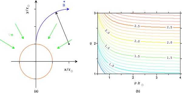
Physically, non-radial curved magnetic field lines (and hence the paths for the type-III-producing electrons) will reduce the apparent value of the power-law index, αapp, because the beam takes longer to reach a given r for a given density profile and beam speed. This effect can be quantitatively estimated as follows. Consider a simple model in which the plasma density depends only on the radial distance, i.e., it is spherically symmetric, and the corresponding plasma frequency can be described by a power law, with fp ∝ r−α. We assume further that the source of type III emission appears first near the solar surface, where the magnetic field is closely radial, and then moves along the curved magnetic field line and the measurements are performed in the frequency range occupying 1 octave, i.e., fmax /fmin = 2. For simplicity, consider the case where the configuration of the magnetic field in the region of interest can be described by one parameter—the curvature of the magnetic field line. In other words, magnetic field lines can be approximated by circular arcs of the same curvature. Without significant loss of generality, we can assume that the emission at the highest frequency is generated just above the Sun, where the field lines are perpendicular to the solar surface (see Figure 6(a)). Then, we can take advantage of the procedure that was used for experimental data processing and thereby determine the apparent power-law index αapp for "observed" frequencies for any particular values of the index α and radius of curvature of the magnetic field line. The results of these numerical simulations are shown in Figure 6(b).
Figure 6. (a) Geometrical model for estimating the effects of magnetic field line curvature on the frequency-time dependence of coronal type III radio bursts. The Sun is shown by the red (gray in the print version) circle centered at the origin. Green (gray in print) arrows show the direction of the plasma density gradient. The blue line (black in print) shows the magnetic field line which is approximated by the arc, with the radius vector shown by a black arrow. (b) The contour plot of apparent power-low indices αapp vs. the real power-low index α for radial dependence of the plasma frequency and the radius of curvature of the magnetic field line, ρ, normalized to the solar radius r☉.
Download figure:
Standard image High-resolution image
It is easily seen that the best index αapp is always smaller than α and that the difference is substantial for ρ < 2 r☉, where ρ is the radius of curvature of the magnetic field line. From Figure 6(b), it follows that for α = 3 and ρ>0.5 r☉ the minimum value of αapp is about 2, so it is impossible to get αapp = 1. With bigger curvature, field lines will go back to the Sun's surface before f = fmax /2. Hence, the effects of curvature of magnetic field lines, although significant, are not sufficient to explain the observed wind-like indices in almost all cases studied. This leads to the conclusion that such small values of α in our type III radio observations provide convincing evidence for the existence of "wind-like" regions within ∼1 r☉ above the photosphere.
Wind-like indices α in a vicinity of 1 will be observed in cases of conical outflows with constant plasma speed, in particular in the case of spherical plasma expansion. The cone vertices do not necessarily coincide with the center of the Sun. Simple considerations based on equation of continuity show that α = 1 will be observed for any conical flow with constant speed (Cairns et al. 2009). However, to explain lower power-law indices, it is necessary to reject the assumption of constant flow speed and/or conical geometry.
For simplicity, consider a small flux tube with variable cross-sectional area, S, and axis in the radial direction. From the continuity equation for time-stationary flows it follows that f2p(r) v(r) S(r) = const, hence, fp ∝ v−1/2S−1/2. If the plasma speed v is constant and the flow is conical, S(r) ∝ (r − r0)2, it immediately follows that fp ∝ (r − r0)−1. Generally, however, the observed power-law index depends on the profiles of both the plasma speed and the cross-sectional area of the flow tube, i.e., on how these vary with r. In a simple case when  and
and  , these two factors are additive:

with αv>0 corresponding to accelerating plasma outflow, while αv < 0 means that the plasma decelerates with increasing r. From Equation (4), it is easily seen that decreased values of α could be observed if the plasma decelerates and/or cross section of the flow tube increases more slowly than it does in the case of conical flow. Under typical conditions, the effect of slowly varying cross-sectional area of the flow tube is probably dominating, while the contribution from the curvature of the magnetic field lines is expected to be relatively smaller and deceleration (if any) is probably negligible. Indeed, there are many observations (e.g., White et al. 1991; White 2004) indicating that in the corona above the active region the magnetic field can be very strong, ∼2000 G or more, these values are known to be typical for sunspots. It means that flow tubes may expand slowly with height above the photosphere.
6. CONCLUSIONS
Solar type III radio bursts are produced near the local electron plasma frequency fp and its harmonic 2fp by relatively low-energy electron beams at a speed of about c/3, where c is the speed of light (e.g., Suzuki & Dulk 1985). They are commonly observed whenever there is a moderately bright active region on the visible side of the Sun. Most frequently, the bursts occur in groups of 10 or more. These bursts have dynamic spectra with frequency rapidly falling with time, the typical duration of the coronal burst being about 1–3 s.
In the present paper, 37 well-defined coronal type III radio bursts (40–400 MHz) are analyzed. It is found that the dependence of the central frequency of the emission on time can be fitted to a power-law model, f ∝ (t − t0)−α, with α in the range from 0.2 to 7 or larger, with the mean and median values of α equal to 1.2 and 0.5, respectively. Most events, 84%, have α ⩽ 1.2. If the speed of the electron beam is constant and the effect of curvature of the magnetic field lines is negligible, it follows herefrom that the plasma density scales as n(r) ∝ (r − r0)−β with the corresponding mean and median values for plasma density indices β ≈ 2α being 2.4 and 1.0, respectively. These findings provide strong evidence that the density profile in the type III source regions within about 1 solar radius above the photosphere is quite often more gently sloping than could be expected from the existing empirical coronal models (e.g., Baumbach 1937; Allen 1947; Saito et al. 1977; Leblanc et al. 1998), substantiate and extend the results of the earlier case studies by Cairns et al. (2009). In the case of negligible plasma acceleration and stationary conical flow, from the mass conservation it follows that the plasma density will decrease as r−2 and α = 1, like in the solar wind. Several events are found with such a wind-like dependence of burst frequency on time. Smaller power-law indices could result from the effects of non-conical geometry of the plasma flow tubes and/or the curvature of the magnetic field lines. The effects of curvature of the magnetic field lines are shown to be not strong enough to explain the observed low power-law indices. Only 7 out of 37 events (18%) are shown to be consistent with the above-mentioned empirical coronal models. In addition, a strong tendency is found for bursts from the same group to have similar power-law indices, thereby favoring the hypothesis that they are produced by the same source region.
In summary, the gently sloping coronal density profiles found in the present paper are inconsistent with well-known coronal density models. This inconsistency indicates that further thorough investigations of observational data are required in order to estimate plasma density and velocity profiles in the solar corona. However, these studies are beyond the scope of the present paper.
We thank the Australian Research Council and German DLR for funding.