


ABSTRACT
We investigate the characteristic radiative efficiency  , Eddington ratio λ, and duty cycle P0 of high-redshift active galactic nuclei (AGNs), drawing on measurements of the AGN luminosity function at z = 3–6 and, especially, on recent measurements of quasar clustering at z = 3–4.5 from the Sloan Digital Sky Survey. The free parameters of our models are , λ, and the normalization, scatter, and redshift evolution of the relation between black hole (BH) mass MBH and halo virial velocity Vvir. We compute the luminosity function from the implied growth of the BH mass function and the quasar correlation length from the bias of the host halos. We test our adopted formulae for the halo mass function and halo bias against measurements from the large N-body simulation developed by the MICE collaboration. The strong clustering of AGNs observed at z = 3 and, especially, at z = 4 implies that massive BHs reside in rare, massive dark matter halos. Reproducing the observed luminosity function then requires high efficiency and/or low Eddington ratio λ, with a lower limit (based on 2σ agreement with the measured z = 4 correlation length) ≳ 0.7λ/(1 + 0.7λ), implying ≳ 0.17 for λ>0.25. Successful models predict high duty cycles, P0 ∼ 0.2, 0.5, and 0.9 at z = 3.1, 4.5, and 6, respectively, and they require that the fraction of halo baryons locked in the central BH is much larger than the locally observed value. The rapid drop in the abundance of the massive and rare host halos at z > 7 implies a proportionally rapid decline in the number density of luminous quasars, much stronger than simple extrapolations of the z = 3–6 luminosity function would predict. For example, our most successful model predicts that the highest redshift quasar in the sky with true bolometric luminosity L > 1047.5 erg s−1 should be at z ∼ 7.5, and that all quasars with higher apparent luminosities would have to be magnified by lensing.
Export citation and abstract BibTeX RIS
1. INTRODUCTION
The masses of the central black holes (BHs) in local galaxies are correlated with the luminosities, stellar and dynamical masses, and velocity dispersions of the galaxies in which they reside (e.g., Magorrian et al. 1998; Ferrarese & Merritt 2000; Gebhardt et al. 2000; McLure & Dunlop 2002; Marconi & Hunt 2003; Häring & Rix 2004; Ferrarese & Ford 2005; Greene & Ho 2006; Graham 2007, 2008; Hopkins et al. 2007a). The MBH–σ relation, together with the observed correlation between outer circular velocity and central velocity dispersion measured by several groups (e.g., Ferrarese 2002; Baes et al. 2003; Pizzella et al. 2005; Buyle et al. 2006), implies a mean correlation between BH mass and the mass or virial velocity of the host galaxy's dark matter halo, although with a possibly large scatter (e.g., Ho 2007a, 2007b). Recent observational studies have attempted to constrain the evolution of the BHs and their host galaxies, by measuring the MBH–σ relation at 0 < z ≲ 3, finding only tentative evidence for larger BHs at fixed velocity dispersion or stellar mass (e.g., McLure et al. 2006; Peng et al. 2006; Shields et al. 2006; Treu et al. 2007; Shankar et al. 2009a) with respect to what is observed locally. However, such an evolution is difficult to detect given the limited sampling and bias effects involving these measurements (e.g., De Zotti et al. 2006; Lauer et al. 2007; Ho 2007a). Probing this evolution becomes even more difficult at z > 2 because luminous active galactic nuclei (AGNs) substantially outshine their hosts.
Another way to probe the evolution of BHs and their host galaxies comes from clustering. Since more massive halos exhibit stronger clustering bias (Kaiser 1984; Mo & White 1996), the clustering of quasars provides an indirect diagnostic of the masses of halos in which they reside (Haehnelt et al. 1998; Haiman & Hui 2001; Martini & Weinberg 2001; Wyithe & Loeb 2005), which in turn can provide information on BH space densities, on duty cycles and lifetimes, and, indirectly, on the physical mechanisms of black hole feeding. Measuring the clustering as a function of redshift and quasar luminosity probes the relation between AGN luminosity and host halo mass, thus constraining the distributions of Eddington ratios and radiative efficiencies which govern the accretion of BHs at different epochs and in different environments. The strong clustering of quasars at z > 3 recently measured by Shen et al. (2007, hereafter S07) in the Sloan Digital Sky Survey (SDSS; York et al. 2000) quasar catalog (Richards et al. 2002; Schneider et al. 2007) implies that the massive BHs powering these quasars reside in massive, highly biased halos.
The classical modeling of quasar clustering by Haiman & Hui (2001) and Martini & Weinberg (2001) assumes a mean value for the duty cycle and derives the relation between quasar luminosity and host halo mass by monotonically matching their cumulative distribution functions. White et al. (2008, hereafter WMC) have applied this method to the S07 measurements, concluding that the strong clustering measured at z ∼ 4 can be understood only if quasar duty cycles are high and the intrinsic scatter in the luminosity–halo relation is small. In this paper, we take a further step by jointly considering the evolution of the BH–halo relation and the BH mass function, as constrained by the observed AGN luminosity function and clustering. We examine constraints on the host halos, duty cycles, radiative efficiencies, and mean Eddington ratios of massive BHs at z > 3, imposed by the clustering measurements of S07 and by a variety of measurements of the quasar luminosity function at 3 ⩽ z ⩽ 6 (e.g., Kennefick et al. 1995; Pei 1995; Fan et al. 2001, 2004; Barger et al. 2003; Wolf et al. 2003; Hunt et al. 2004; Barger & Cowie 2005; La Franca et al. 2005; Nandra et al. 2005; Cool et al. 2006; Richards et al. 2006a; Bongiorno et al. 2007; Fontanot et al. 2007; Shankar & Mathur 2007; Silverman et al. 2008; Shankar et al. 2010; F. Shankar et al. 2010, in preparation).
Our method of incorporating luminosity function constraints is simple. We assume the existence of a relation between BH mass MBH and halo virial velocity Vvir at high redshift and assume that the slope of this relation is the same as observed locally, but leave its normalization, redshift evolution, and scatter as adjustable parameters. Since the halo mass function is predicted from theory at every redshift, the evolution of the BH mass function follows once the MBH–Vvir relation is specified. This growth of BHs is then used to predict the AGN luminosity function, in terms of the assumed radiative efficiency  and Eddington ratio λ = L/LEdd of BH accretion, which can be compared to observations. This method inverts the "continuity equation" approach to quasar modeling, in which one uses the observed luminosity function to compute the implied growth of the BH mass function (e.g., Cavaliere et al. 1971; Small & Blandford 1992; Yu & Tremaine 2002; Steed & Weinberg 2003; Marconi et al. 2004; Shankar et al. 2004; Yu & Lu 2004; Shankar et al. 2009b, hereafter SWM; Shankar 2009).
We make no specific hypothesis about the mechanisms that trigger high-redshift quasar activity. Our model simply assumes that a relation between MBH and Vvir exists and that it is maintained by mass accretion that produces luminous quasar activity, assuming no significant time delay between the two. As detailed below, simultaneously matching the observed luminosity function and the S07 clustering measurements, especially their z = 4 correlation length, is in general quite difficult. Moderately successful models must share the common requisites of having low intrinsic scatter in the MBH–Vvir relation and a high value of the ratio /λ. Although these findings are affected by the model adopted to compute the halo bias factor, we will show that they do not otherwise depend on the details of our modeling and can be understood in simple, general terms.
The mass function and clustering bias of rare, massive halos at high redshift are crucial inputs for our modeling. We therefore test existing analytic formulae for these quantities against measurements from the large N-body simulation developed by the MICE collaboration, which uses 109 particles to model a comoving volume of 768 h−1 Mpc on a side.
Throughout this paper, the following cosmological parameters have been used, consistent with the best-fit model to WMAP5 data (Spergel et al. 2007): Ωm = 0.25, ΩL = 0.75, σ8 = 0.8, n = 0.95, h ≡ H0/100 km s−1 Mpc−1 = 0.7, and Ωb = 0.044.
2. MODEL
2.1. AGN Bias and Luminosity Function
In the local universe, the masses of BHs are tightly correlated with the velocity dispersion σ of their parent bulges (e.g., Ferrarese & Merritt 2000; Gebhardt et al. 2000; Tremaine et al. 2002). This relation has been recently re-calibrated by Tundo et al. (2007) as
where we denote the average BH mass at a fixed σ as  . The bulge velocity dispersions are in turn correlated with large-scale circular velocities (Ferrarese 2002; see also Baes et al. 2003; Pizzella et al. 2005):

with σ and Vc measured in km s−1. For a flat rotation curve, the disk circular velocity is equal to the halo virial velocity Vvir. Departures from isothermal halo profiles, gravity of the stellar component, and adiabatic contraction of the inner halo can alter the ratio Vvir/Vc, but the two quantities should remain well correlated nonetheless (e.g., Mo et al. 1998; Mo & Mao 2004, and references therein). Thus, the correlations (1) and (2) imply a correlation between BH mass and halo virial velocity, although we should expect the MBH–Vvir relation to have a larger scatter than the observed MBH–σ relation (e.g., Ho 2007b).
As mentioned in Section 1, the models we shall construct assume that BHs at z > 3 lie on an MBH–Vvir relation of similar form. We parameterize this relation as
which corresponds to Equations (1) and (2) with Vvir replacing Vc. We define α as the normalization of the MBH–Vvir relation at z = 3.1, which corresponds to the mean redshift in the lower subsample of S07. The factor α allows both for an offset between the z = 3.1 and z = 0 relations and for a ratio Vvir/Vc ≠ 1 at z = 0. For example, typical disk galaxy models (e.g., Mo et al. 1998; Seljak 2002; Dutton et al. 2007; Gnedin et al. 2007) have Vc/Vvir ≈1.4–1.8 at z = 0, which would imply normalizations α ≈ 5–15 for Equation (3) at z = 0 because of the steep power of velocity. Note that none of our results depend on the z = 0 normalization of the  relation because we use only high-redshift data in this paper. In addition, we allow redshift evolution in the MBH–Vvir relation at z > 3.1 through the index γ.
The relation between the halo virial velocity Vvir and the halo virial mass M is
where the mean density contrast (relative to critical) within the virial radius Rvir is Δ = 18π2 + 82d − 39d2, with d ≡ Ωm(z) − 1, and Ωm(z) = Ωm(1 + z)3/[Ωm(1 + z)3 + ΩΛ] (Bryan & Norman 1998; Barkana & Loeb 2001). In terms of halo mass, Equation (3) corresponds to
We assume the presence of a scatter about this mean relation, with a log-normal distribution and a dispersion Σ in the logarithm of BH mass at fixed Vvir.
Given the theoretically known halo mass function, we compute the BH mass function via the convolution
with

where Σ is the log-normal scatter in MBH at fixed halo mass, x = MBH or M, and ns(x, z)dx is the comoving number density of BHs/halos (for subscript s = BH or s = h) in the mass range x → x + dx, in units of Mpc−3 for H0 = 70 km s−1 Mpc−1. The units of Φs are comoving Mpc−3 per decade of mass. We convert to these units in order to compare with the data on the AGN luminosity function.
The quasar luminosity function Φ(L, z), expressed in the same units as Φs(x, z), is modeled according to a simple prescription where BHs can be in only two possible states: active or inactive. All BHs that are active accrete with a single value of the radiative efficiency, , and of the Eddington ratio, λ = L/LEdd, where L is the bolometric luminosity and
is the Eddington luminosity (Eddington 1922). The growth rate of an active BH of mass MBH is  MBH/tef, where the e-folding time is (Salpeter 1964)
where f = /(1 − ), and the radiative efficiency is ![$\epsilon =L(1-\epsilon)/[\dot{M}_{\rm BH}c^2]$](https://content.cld.iop.org/journals/0004-637X/718/1/231/revision1/apj297014ieqn5.gif) . (Radiative efficiency is conventionally defined with respect to the mass inflow rate
. (Radiative efficiency is conventionally defined with respect to the mass inflow rate  , and the BH mass growth rate
  is smaller by a factor 1 − because of radiative losses).
Once the parameters α and γ of the MBH–Vvir relation are specified, the growth of ΦBH(MBH, z) is determined by the (theoretically calculable) evolution of the halo mass function nh(M, z). We compute the AGN luminosity function assuming that this growth is produced by accretion with radiative efficiency and Eddington ratio λ. This method inverts a long-standing approach to modeling AGN and BH evolution in which one calculates the growth of the BH mass function implied by the observed luminosity function using a "continuity equation,"
(see, e.g., Cavaliere et al. 1971; Small & Blandford 1992; Yu & Tremaine 2002; Marconi et al. 2004; SWM). Here, we ignore the impact of BH mergers in the evolution of the BH mass function, because the BH mass growth via mergers is relatively small, as we show in detail in the Appendix.
Knowing ΦBH(MBH, z), we can invert Equation (10) to obtain the luminosity function
In practice, we integrate Equation (11) up to BH masses of log MBH/M☉ = 11. Equation (11) assumes a strictly monotonic, scatter-free relation between AGN luminosity and BH mass. Therefore, in our models the only source of scatter between AGN luminosity and halo mass is the scatter in the MBH–Vvir relation. However, provided that the L–Vvir scatter is fairly small (as we find it must be to explain the observed clustering), we expect that it makes little difference whether it arises from scatter in MBH or scatter in λ.
The average growth rate of all BHs (active and inactive) of mass MBH is  , where the duty cycle P0 is the probability that a BH is in the active state. In models with a single value of λ, the duty cycle is simply the ratio of the luminosity function to the mass function,
where  . A physically consistent model must have P0 ⩽ 1 for all MBH and z, and can be directly computed from Equations (6) and (11).
In addition to the AGN luminosity function, we test our models against the clustering measurements of S07, specifically their reported values of the AGN correlation length r0. We calculate these correlation lengths from the condition

where ξ(r0) is the Fourier transform of the linear power spectrum, D(z) is the linear growth factor of perturbations, and  is the mean clustering bias of AGN shining above a luminosity threshold Lmin at redshift z, given by (Haiman & Hui 2001)
The minimum luminosity Lmin(z) in Equation (14) is a bolometric quantity, while the S07 bias is measured above a redshift dependent, K-corrected Mi magnitude. To convert from magnitudes to bolometric luminosities, we first convert to B magnitudes assuming MB = Mi(z = 2) + 0.804 (Richards et al. 2006b), and then adopt an average bolometric correction of CB = 10.4, with L = CBLBνB, where νB is the frequency at the center of the B band (at wavelength 4400 Å). Because our models assume a single Eddington ratio λ, b(L,z) is just equal to the bias b(MBH, z) of BHs of mass MBH = L/lλ. The latter is computed from the b(M, z) of halos of mass M using the model relation between MBH and M(z) (Equation (5)). Including the log-normal scatter of width Σ, the BH bias is
We discuss our choice of b(M,z) in Section 2.2.
In summary, the free parameters of our model are as follows.
- 1.the normalization constant α in the MBH–Vvir relation,
- 2.the parameter γ which regulates the redshift evolution [(1 + z)/4.1]γ of this relation,
- 3.the mean Eddington ratio λ of active BHs,
- 4.the log-normal scatter Σ in MBH at fixed Vvir, and
- 5.the radiative efficiency of BH accretion.
The predicted bias in these models is completely independent of the assumed radiative efficiency (when other parameters are held fixed), since the efficiency does not affect the relation between luminosity and halo mass.
2.2. Mass Function and Halo Bias
The high-redshift quasars used by S07 and our study are believed to reside in very rare halos with M ∼ 1012–1013 h−1 M☉ at redshifts z = 3–6. While extensive work has been done to determine the abundances and clustering of halos at z < 3, testing the accuracy of simple analytic formulae against predictions from cosmological numerical simulations of structure formation, this work has not been extended to the high-redshift (z ∼ 3–6), rare massive halos we are interested in here (but see Reed et al. 2007, 2009).
We perform this test here, using a large N-body simulation from the MICE collaboration with 10243 particles and cubic volume of side Lbox = 768 h−1 Mpc, for the cosmological parameters listed in Section 1. The initial conditions were set at z = 50 using the Zel'dovich approximation, with an input linear power spectrum given by the analytic fit of Eisenstein & Hu (1999). The subsequent gravitational evolution was followed using the Tree-SPH code Gadget-2 (Springel et al. 2005). Halos were identified using the friends-of-friends (FoF) algorithm (Davis et al. 1985), with linking length equal to 0.164 times the mean interparticle density. The minimum halo mass resolved in the simulation is Mmin = 6 × 10¹¹ h−1 M☉, with a minimum of 20 particles per halo.
The halo mass function from the simulation is shown as solid symbols in Figure 1 (filled circles, filled squares, open triangles, and open circles indicate the abundances of halos at redshifts z = 3, 4, 5, and 6, respectively). We plot the quantity f(M, z) = nh(M, z)dM, where nh(M, z)dM is the number of halos per comoving volume at redshift z with mass between M and M + dM. The dashed and solid lines are the analytical models from Sheth & Tormen (1999, ST hereafter) and Jenkins et al. (2001; their Equation (B2)), respectively, plotted at the same redshifts. To better display the difference between simulations and models, the lower panel of Figure 1 shows the fractional deviation with respect to the Jenkins et al. (2001) fit, with all the lines and symbols as in the upper panel.
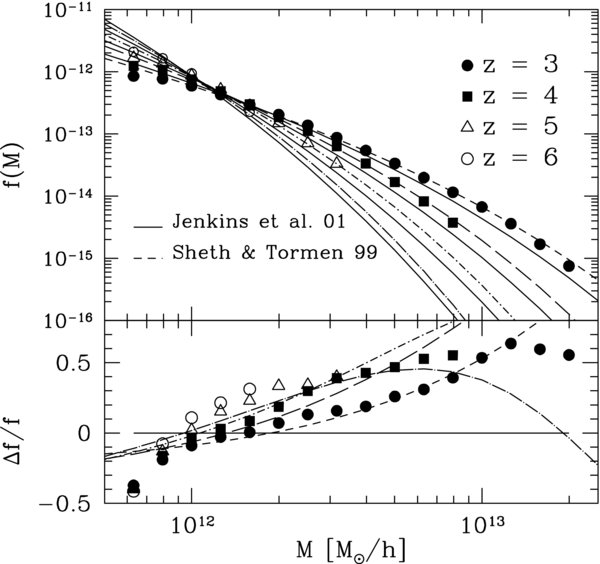
Figure 1. Halo mass function: comparison between N-body measurements and analytic fits. Upper panel: measured mass functions for FoF halos identified at redshifts 3 (filled circles), 4 (filled squares), 5 (open triangles), and 6 (open circles) in our simulation are in better agreement with Sheth & Tormen (1999) (discontinuous lines) rather than the Jenkins et al. (2001, solid lines) analytic fits. Fits are displayed for the same redshifts as measurements in the simulation: from z = 3 (upper lines) to z = 6 (bottom lines). Lower panel: fractional deviations of the measured mass functions (symbols as in upper panel) and the Sheth & Tormen predictions (discontinuous lines as above) with respect to the Jenkins et al. fit (solid line).
Download figure:
Standard image High-resolution imageOverall, we find that the ST model fits the simulations in the range z = 3–5 within 15% accuracy, while for z = 6 the error is about 20% in the range log(M/M☉ h−1) = 12–13. We use the ST model in the rest of the paper, because the Jenkins et al. (2001) formula is clearly a worse fit to the simulation results in the regime of interest.
As mentioned before, the halos we are interested in are rare, and studying their clustering properties is therefore difficult. This "rarity" can be quantified by means of the peak height ν = δc/σ(M, z), which characterizes the amplitude of density fluctuations from which a halo of mass M forms at a given redshift z (here, δc = 1.686, and σ(M, z) is the linear overdensity variance in spheres enclosing a mean mass M).
Gao et al. (2005) computed the halo bias using the Millennium Simulation (Springel 2005) at redshifts z = 0–5, but only for halos collapsing from fluctuations up to 3σ. Angulo et al. (2008) measured the bias of ∼4.5σ halos, but only for z ⩽ 3. In the context of the reionization of the universe, Reed et al. (2009) studied the bias of <4σ halos at redshift z > 10. Additional work on halo bias is presented in Seljak & Warren (2004), Cohn & White (2008), Basilakos et al. (2008), and references therein. In this section, we extend these studies to the regime of our interest, namely, 3σ–5σ halos at z = 3–6.
We computed the bias factor of halos from simulation outputs at z = 3, 4, 5, 5.5, and 6. At each output, we divided the halo catalog into three mass bins of equal separation in log M, log(M/M☉ h−1) = 11.75–12.25, 12.25–12.75, and 12.75–13.25. We then measured the ratio of correlation functions b = ξhm(r)/ξmm(r) at 10 bins of equal width in log r in the range 8 h−1 Mpc ⩽ r ⩽ 38 h−1 Mpc (where ξhm is the two-point halo–matter correlation and ξmm the matter–matter correlation function). The bias was computed as the mean of these values, and their variance was used as a rough estimate of the error. We warn that this error indicator may be underestimating the true uncertainty in our measurements, since the correlation function errors are correlated in neighboring radial bins (although this effect is less severe in the presence of shot noise).
We analyze halo bias from ξhm instead of  to overcome the intrinsic noise in the latter quantity due to low halo abundance (see also Cohn & White 2008). The two definitions may differ owing to stochasticity in the halo–matter relation. However, we have tested that both measures yield consistent results (within error bars), while the variance among different bins is reduced by about 50% when using ξhm (details of this comparison are given in the Appendix).
In addition to the 8–38 h−1 Mpc measurements, we have computed bias using the ξ20 measure adopted by S07 and using the range 30–60 h−1 Mpc. These results are reported in the Appendix. We find no evidence for scale dependence of the halo bias outside our statistical uncertainties, but the issue deserves further investigation in future work (Reed et al. 2009).
In Figure 2, we show the results for the halo bias at high redshift as obtained from the MICE simulation (with symbols corresponding to different redshifts as labeled in the figure). The left panel depicts the bias as a function of halo mass for various redshifts; the lines are predictions from the ellipsoidal collapse formula of Sheth et al. (2001),
where a = 0.707, b = 0.5, c = 0.6, ν = δc/σ(M, z), and δc = 1.686. The right panel shows instead the bias as a function of peak height ν, in terms of which the predictions for all redshifts coincide (Equation (16)). In addition to Equation (16), we also include in this figure the fitting formula derived by Jing (1998; see also Mo & White 1996).
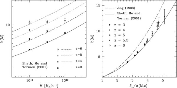
Figure 2. Halo bias estimated from ξhm/ξmm on scales 8–38 h−1 Mpc−1. The symbols represent the results from a MICE simulation for different redshifts and halo masses as labeled (see the text for details). In the left panel, we show halo bias vs. mass and the corresponding prediction of Sheth et al. (2001). The right panel shows bias vs. peak height ν = δc/σ and includes the Jing (1998) fit (which mostly coincides with Mo & White (1996) expression at these values of ν). The Sheth et al. (2001) bias works well overall, but it underestimates the results from the simulation at high redshifts. Jing's fit, on the other hand, overpredicts the measurements for all masses and redshifts studied by as much as 15%–20%.
Download figure:
Standard image High-resolution imageFigure 2 shows that Jing's (1998) fit overestimates the bias at all redshifts and masses studied at the 15%–20% level. The Sheth et al. (2001) prescription is in good agreement with the simulation for the lower fluctuations (ν ⩽ 4) that correspond to halos of mass 3 × 10¹² h−1 M☉ at z ⩽ 5, but it underestimates the bias of the rarest halos of ν>4 by up to 10%. As noted by Crocce et al. (2006), transients from the Zel'dovich dynamics generally used to set up the initial conditions lead to systematically high values for halo bias. This effect manifests itself more strongly in rare halos, so the discrepancy with Sheth et al. (2001) in this regime could be a numerical artifact rather than inaccuracy of the analytic model. Our conclusions are in good agreement with existing work on halo bias covering slightly different regimes (and mentioned at the beginning of this section). Therefore, we will use the Sheth et al. (2001) model for the bias and discuss in Section 3.2 the impact that adopting Jing's (1998) bias formula would have on our conclusions.
3. RESULTS
3.1. Comparison to Observational Data
3.1.1. The Data
In this section, we compare our model predictions with the available data on quasar clustering and the AGN luminosity function. This comparison is made in Figure 3, where the upper left panel shows results for the AGN correlation length and the other three panels show the luminosity function at three different redshifts: z = 3.1, z = 4.5, and z = 6.
Figure 3. Upper left panel: model predictions for the quasar correlation length r0 as a function of redshift for different values of the input parameters, as labeled, computed above the luminosity threshold taken from Figure 1 of Richards et al. (2006a). The diamonds and triangles are the Shen et al. (2007) clustering measurements, corrected to H0 = 70 km s−1 Mpc−1, calibrated on their "good" and total sample, respectively (see Shen et al. for details). Upper right panel: model predicted luminosity functions at z = 3.1, for the same set of models; the data are the collection from Shankar et al. (2009b) and Shankar & Mathur (2007), to which we refer the reader for details. Lower left panel: model predicted luminosity functions at z = 4.5. Lower right panel: model predicted luminosity functions at z = 6.0. The open and filled circles in the last three panels represent the AGN luminosity function before and after obscuration correction, respectively (see the text for details). The vertical, thick, dotted lines in this and the following figures mark the bolometric luminosity of L = 8 × 1046 erg s−1, taken as the approximate luminosity threshold of the clustering measurements. Only data in the luminosity function above this threshold have been taken into account in the χ2-fitting.
Download figure:
Standard image High-resolution imageThe data on the clustering are taken from S07, who have recently extended beyond z ∼ 3 previous measurements of the quasar clustering at lower redshifts from the Two Degree Field Quasar Redshift Survey (Porciani et al. 2004; Croom et al. 2005; Porciani & Norberg 2006; da Ângela et al. 2008; Mountrichas et al. 2009) and SDSS (e.g., Myers et al. 2007; Strand et al. 2008; Padmanabhan et al. 2009). All the symbols in the upper left panel of Figure 3 represent the SDSS measurements averaged over sources with redshifts 2.9 ⩽ z ⩽ 3.5 and z ⩾ 3.5. The diamonds and triangles refer to the S07 results extracted for the "good" and whole samples, respectively.5 Following S07, we take z = 3.1 and z = 4.0 as the effective measurement redshifts for the two redshift bins.
The S07 clustering measurements are for optically identified AGNs only. However, the growth of BHs is connected to the total luminous output of the AGN population, not that of obscured or unobscured sources alone. We consider obscuration here as a random variable not linked with the large-scale clustering of AGNs, so that the correlation length of obscured AGNs is the same as that of unobscured ones of the same bolometric luminosity. This assumption is plausible regardless of whether obscuration is principally a geometrical effect or an evolutionary phase.
Following SWM, we take the AGN luminosity function at the mean redshifts of z = 3.1, 4.5, and 6, where most of the high-redshift optical and X-ray data sets collected in SWM and Shankar & Mathur (2007, and references therein) are concentrated. We then adopt6 Equation (4) of Hopkins et al. (2007b) to re-normalize the luminosity function to include obscured sources, assuming the obscuration is independent of redshift. However, because the obscuration correction may suffer from significant uncertainties, even up to a factor of a few (e.g., Ueda et al. 2003; La Franca et al. 2005; Tozzi et al. 2006; Gilli et al. 2007; Hopkins et al. 2007b), when comparing model predictions to the bolometric luminosity function we will also include uncertainty in the obscuration correction as a source of systematic error to be added to the statistical error of the luminosity function measurements. In Figure 3, the filled and open circles show the luminosity function with and without obscuration corrections, respectively.
3.1.2. General Properties of the Models
Figures 3 and 4 illustrate the dependence of model predictions on the adopted parameters. In general terms, we can understand the interplay between the different parameters by combining Equations (5), (9), and (11). Before examining the impact of individual parameter changes, we should note that there is one exact degeneracy within our family of models, if the luminosity function and correlation length are the only constraints. If we lower the Eddington ratio by a factor of Γ but raise the MBH–Vvir normalization α by the same factor, then the host halo mass at a given quasar luminosity is unchanged, so the predicted clustering is unchanged. All BH masses are larger by a factor Γ, and so are their average growth rates required to match the evolving halo mass function, but if we lower the efficiency factor f = /(1 − ) by the same factor Γ, then the luminosity function implied by this growth is unchanged. Our analysis therefore cannot constrain λ and f individually, but it can provide interesting constraints on the ratio f/λ.
Figure 4. Impact of changing the scatter Σ or evolution parameter γ of the MBH–Vvir relation. The format is as in Figure 3, and the adopted model parameters are labeled in the upper left panel. Increasing scatter worsens the match to the clustering data, and lowering γ worsens the match to luminosity function evolution.
Download figure:
Standard image High-resolution imageIn Figure 3, all models have evolution parameter γ = 1.0 and a tight correlation between MBH and M, with Σ = 0.1 dex. Solid lines in each panel show the predictions of a "reference model" with radiative efficiency = 0.15, Eddington ratio λ = 0.25, and a normalization of the MBH–Vvir relation α = 1.1. This model matches the S07 value of r0 at z = 3.1. At z = 4, it is consistent with S07's measurement from the full quasar sample, but it falls below the "good" sample measurements by about 2σ. This model is in fairly good overall agreement with the bright end of the AGN luminosity function at all redshifts, though it is somewhat low at z = 4.5.
In general, all our models tend to overpredict the faint end of the AGN luminosity function below L ∼ 1046 erg s−1 at z = 3.1 and, more severely, at z = 4.5. These behaviors suggest that one or more of the model assumptions break down at lower luminosities. For example, the assumption of a constant λ and may not be valid. Alternatively, the assumed monotonic relation between BH mass and halo mass could break down in this regime (see, e.g., Tanaka & Haiman 2009). However, these hypotheses cannot be tested with the present data because the bias measurements by S07 do not probe luminosities fainter than L ⩽ 1047 erg s−1, which is where our models start diverging from the data. We therefore do not attempt to reproduce the faint end of the AGN luminosity function with our models in this work.
We now examine the consequences of varying each of the five model parameters, as listed at the end of Section 2.1. We first consider lowering the Eddington ratio to λ = 0.1, keeping the other parameters fixed. Since the BH abundances and their growth rates are fixed by their correspondence to halos, the duty cycles must increase as the inverse of λ to compensate for the lower accretion rates during the active phase, thereby keeping the average volume emissivity from quasars constant. The results for this case are shown as the dotted line in Figure 3. A better match to the high observed clustering amplitude is clearly achieved, because the observed quasars correspond to more massive BHs and rarer halos. However, the fit to the luminosity function is worse because the abundance of the most luminous quasars is underpredicted. Low values of the Eddington ratio are also disfavored by other observational (e.g., Bentz et al. 2006; Kollmeier et al. 2006; Kurk et al. 2007; Netzer & Trakhtenbrot 2007; Shen et al. 2008) and theoretical studies (Shankar et al. 2004; Lapi et al. 2006; Volonteri & Rees 2006; Li et al. 2007; SWM; Di Matteo et al. 2008).
When the MBH–Vvir normalization α is lowered (dashed curve in Figure 3), the effect is simply to lower the BH masses and quasar luminosities at fixed abundance. At fixed quasar luminosity, the clustering increases owing to the greater mass of the associated halos, but the decrease in abundance prevents a good match to the data. The dot-dashed curve illustrates the triple degeneracy described at the beginning of this section: a different set of (λ,α,) values whose predictions are nearly identical to those of the reference model.
Figure 4 shows the effect of varying the scatter Σ or the evolution parameter γ of the MBH–Vvir relation. A low scatter maximizes the bias for a given set of other parameters, so low scatter is favored to reproduce the high values measured for r0 at these redshifts (see also WMC). On the other hand, semi-empirical studies and AGN theoretical modeling support a significant intrinsic scatter for the MBH–M relation at redshifts z ≲ 3 (e.g., Lapi et al. 2006; Haiman et al. 2007; Myers et al. 2007; Gultekin et al. 2009). Increasing the scatter to Σ = 0.3 (dotted lines), boosts the AGN luminosity function by increasing the number of massive BHs, but it depresses clustering because more quasars at a given L reside in less massive halos. It also slightly flattens the dependence of the predicted r0 on redshift. We then need to lower α or λ to restore the luminosity function and increase r0. However, lowering λ or α would also require higher radiative efficiencies to keep the match to the luminosity function. We also find that models with Σ = 0.3, ≳ 0.25, and α ≲ 0.7 predict more AGNs than BHs, yielding the unphysical condition of P0 > 1 at z > 4.
The parameter γ regulates the amplitude of the model AGN luminosity function at high redshifts relative to that at z = 3.1. Dashed lines in Figure 4 show a model with evolution index γ = 0 and other parameters the same as those of the reference model. Lowering γ maps the same L to higher mass, more biased halos at higher redshifts, steepening the r0–z relation and bringing it closer to the observed trend. However, more massive halos are rarer at higher redshifts, so the predicted AGN luminosity function drops significantly below the data at z = 4.5 and, especially at z = 6. Reproducing the observed luminosity evolution requires positive evolution (γ>0) of the MBH–Vvir relation.
3.1.3. A Closer Comparison
Figure 5 presents a more systematic view of the dependence of clustering and luminosity function predictions on model parameters. Because none of our models reproduce all aspects of the data, and because observational errors may in some cases be dominated by systematic rather than statistical uncertainties, we have taken only a semi-quantitative route to comparing models and measurements. The upper left panel shows models with λ = 0.25, Σ = 0.1, and γ = 1, defining the contour levels of acceptable models on a grid of (α, ) values. The blue and red areas define the regions where the χ2dof for the luminosity is below 3 and 1.5, respectively. Here χ2dof = χ2/N, where N = 45 is the number of points in the luminosity function, which include only those points (from Figure 3) with L ⩾ 8 × 1046 erg s−1, the approximate luminosity threshold of the clustering measurements, marked with vertical, thick, dotted lines in the figures. For comparison, note that the models shown by the dashed and dotted lines in Figure 3 have χ2/N = 5.41 and 18.13, respectively, while the reference model has χ2/N = 1.37. If the data points were independent, then even χ2/N = 1.37 for N = 45 would be an enormous statistical discrepancy, but the systematic uncertainty in the obscuration correction, at least, is highly correlated among points at a given redshift, motivating our rather loose criterion for "agreement." We assign observational errors to each data point equal to the reported statistical error (usually derived from the Poisson error on counts in the bin) summed in quadrature with 50% of the difference between the obscuration corrected and uncorrected luminosity function estimates. This procedure is ad hoc, but it captures the reasonable expectation that the uncertainty on the obscuration correction is of the same order as (but smaller than) the correction itself, and the fact that the scatter among data sets visible in Figure 3 is comparable to the difference between open and filled symbols.
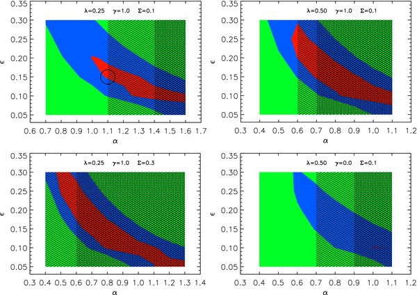
Figure 5. χ2dof per degree of freedom as a function of the radiative efficiency and α, the normalization of the MBH–Vvir relation, with other parameters fixed at the values listed on top of each panel. The blue and red areas define the regions in the –α plane where the χ2dof for the luminosity is below 3 and 1.5, respectively. For the luminosity function, we have used only the data with L ⩾ 8 × 1046 erg s−1, which is the luminosity threshold above which clustering measurements are available. The double-hatched and hatched areas define the regions where the χ2dof for the correlation length at z = 4 is above 6 and 4, respectively. The circle in the upper left panel marks the parameters of our reference model.
Download figure:
Standard image High-resolution imageThe double-hatched and hatched areas define the regions where χ2 = (r0,obs − r0,pred)2/σ2obs, with the S07 value of (r0,obs, σobs) = (24.3, 2.4)h−1 at z = 4.0, is above 6 (i.e., a ≳2.5σ discrepancy) and 4, respectively. Note that the contour plots for the clustering are vertical, given that the predicted clustering strength is independent of the values for the radiative efficiency (see Section 2). We find the constraints from the S07 clustering measurement of (r0,obs, σobs) = (16.9, 1.7)h−1 at z = 3.1 not to be very constraining given that almost all models explored in Figure 5 are consistent with such data at the ≲2σ level. It is clear from Figure 5 that the acceptable models are in general places in the upper left corner of the (α, ) plane, characterized by higher radiative efficiencies and lower values of α for the same quasar luminosity/BH mass, which implies higher halo masses (Equation (5)) and corresponding clustering amplitude.
Examination of Figure 5 reinforces the generality of the points made in our discussion of Figures 3 and 4. The circle in the upper left panel marks our reference model with α = 1.1, γ = 1.0, Σ = 0.1, λ = 0.25, and = 0.15. Note that our reference model is not the best-fit model, as some models characterized by higher radiative efficiency and lower α have an overall lower χ2. However, we preferred to adopt as working models those defined by not too extreme values of the radiative efficiency. Also, the reference model already predicts P0 ≈ 1 at z = 6 (see Figure 8 below), and lowering α reduces the BH space density and pushes P0 above unity. Other models with the same α but different have identical clustering, but the match to the observed luminosity function becomes worse for ⩽ 0.1 and ⩾ 0.25. Lowering α at fixed improves the clustering agreement but quickly makes the luminosity function agreement worse. Raising α to 1.2 or 1.3 slightly improves the luminosity function agreement but worsens the clustering agreement. Raising λ to 0.5 (upper right panel) worsens the agreement with the z = 4 clustering if and α are held fixed. However, because of the three-way degeneracy noted at the beginning of this section, a model with λ = 0.5, = 0.25, and α = 0.5 makes very similar predictions to a model with λ = 0.25, = 0.15, and α = 1.0 (which has f/λ smaller by a factor of ≈2), and we disfavor the higher λ models only on physical grounds because of the high required efficiency. Models with Σ = 0.3 (lower left) yield consistently worse agreement with the z = 4 correlation length unless lower values of α are adopted, but low-α models produce P0 > 1 at high redshifts and require high radiative efficiencies to match the luminosity function. Models with γ = 0.0 (lower right) yield consistently worse agreement with the luminosity function.
Our reference model underpredicts the S07 z = 4 correlation length (the value for "good" fields) by 2.2σ, and it slightly underpredicts the observed luminosity function in the luminosity range corresponding to the S07 quasar sample. If we take these discrepancies as a maximal allowed level of disagreement, then our reference model effectively defines a lower limit on the allowed value of f/λ, at f/λ = 0.7. This conclusion does not depend on our adopted bolometric correction. If we assumed a bolometric correction higher by a factor Γ, then we would require higher λ (by the same factor) for fixed BH masses to match our revised estimate of the bolometric luminosity function. We would also require higher f, again by a factor Γ, to reproduce the observed luminosity function history while building the same BH population. For observationally estimated Eddington ratios λ ≳ 0.25 (Kollmeier et al. 2006; Shen et al. 2008), our limit on f/λ implies ≳ 0.15, significantly higher than the radiative efficiency ≈ 0.1 expected for the disk accretion onto a non-rotating BH.
3.1.4. Varying the Bias
These constraints would be much looser if we adopted the Jing (1998) bias function instead of the Sheth et al. (2001) formula that fits our N-body data. As already discussed in the previous sections, the Jing (1998) formula predicts a significantly higher value of the bias. Therefore, a much larger family of models can match the z = 4 S07 clustering measurements, with no strict requirement for a high f/λ ratio. For example, Figure 6 compares the predictions of the reference model to two alternatives, one with = 0.065 (f/λ ≈ 0.28) and the other with λ = 0.5 (f/λ ≈ 0.22), with r0 calculated using the Jing (1998) formula in all models. The luminosity function predictions of the reference model are unchanged, and all three models yield acceptable agreement with the z = 4 clustering measurement. The low model underpredicts the luminosity function, but the λ = 0.5 model overpredicts it, and lowering to ∼0.1 in this case would yield acceptable agreement. All three models overpredict the z = 3.1 correlation length. With optimal choices of α and λ, one could find models that graze the top of the z = 3.1 error bar and the mean of the z = 4 correlation length while acceptably matching the bright end of the luminosity function (e.g., λ = 0.3, = 0.06, γ = 1, α = 2.3, and Σ = 0.1). Alternatively, one could adopt any of the models shown in Figure 6 but drive down the z = 3.1 clustering by assuming that the scatter Σ grows substantially between z = 4 and z = 3.
Figure 6. Same format as Figure 3, but Jing's (1998) bias formula has been adopted instead of the Sheth et al. (2001) one, and we consider models with lower values of /λ in addition to the reference model (solid line). In the upper left panel, the solid line overwrites the dot-dashed line because the two models have the same black hole mass–halo mass relation.
Download figure:
Standard image High-resolution image3.2. Bias and Duty Cycle Predictions for the Reference Model
Here, we discuss further properties and predictions of a model that simultaneously matches the observed luminosity function and (at the 2σ level) the clustering. For simplicity, all the results presented below are obtained from the reference model, which has (α, Σ, γ, λ, ) = (1.1, 0.1, 1.0, 0.25, 0.15). Figure 7 shows the predicted bias b(L,z) as a function of B-band magnitude; the solid, dashed, and dotted lines correspond to z = 3.1, 4.5, and 6, respectively. Note that b(L,z) now refers to bias at a given luminosity rather than above a given luminosity. The predicted bias increases significantly with luminosity, at variance with what has been observed at lower redshifts z ≲ 2, where evidence for a much flatter behavior of the bias against luminosity has been found (e.g., da Ângela et al. 2008; Myers et al. 2007; Porciani & Norberg 2006; Coil et al. 2007; Mountrichas et al. 2009; Padmanabhan et al. 2009). Note that our prediction applies only to the very bright end of the AGN luminosity function, with L ≳ 8 × 1046 erg s−1; there are no available clustering measurements below this luminosity at z > 3.5.
Figure 7. Predicted bias for our reference model as a function of B-band magnitude at different redshifts, as labeled.
Download figure:
Standard image High-resolution imageWe compute the effective halo mass that corresponds to the quasar hosts at the S07 luminosity thresholds via the relation  . Our reference model yields Meff ∼ 1.1 × 10¹³ h−1 M☉, nearly constant within 3 ⩽ z ⩽ 6. This mass scale is in marginal agreement with what has been inferred from the clustering analysis of large AGN-galaxy surveys at lower redshifts (e.g., Myers et al. 2007; Mountrichas et al. 2009), supporting a roughly constant host halo mass for luminous quasars at all times. Our reference model underpredicts the S07 correlation length at z = 4, so if we used their measured bias we would obtain a somewhat higher Meff at this redshift. In fact, S07 find an effective host halo mass for quasars at z ≳ 3.5 that is a factor of 2 higher than the host halo mass for quasars with 2.9 ⩽ z ⩽ 3.5. Their mean values are Meff = 2.5 × 10¹² h−1 M☉ and 5 × 10¹² h−1 M☉ in the low- and high-redshift bins, respectively, significantly lower than our quoted value, owing to their use of the Jing (1998) bias formula, which yields lower halo masses at fixed bias.
Francke et al. (2008) have recently measured the clustering of 58 X-ray selected AGNs at z ∼ 3 in the Extended Chandra Deep Field South, cross correlating them with a sample of 1385 luminous blue galaxies at the similar redshifts. Their quoted bias is b = 4.7 ± 1.7 corresponding to halos of mass log M/M☉ = 12.6+0.5−0.8, in line with the previous findings by Adelberger & Steidel (2005) derived from optical quasar samples at similar redshifts and luminosities. These studies probe AGNs about 6 mag fainter than those probed by S07, and they seem to support a significant decrease of the bias at lower luminosities. These results would then be in qualitative agreement with our model predictions, but at variance with the flat dependence of quasar clustering on luminosity found at lower redshifts (e.g., Myers et al. 2007; Coil et al. 2007; Padmanabhan et al. 2009). Larger surveys of low-luminosity quasars are needed to reduce the errors on the clustering measurements.
Figure 8 shows the duty cycle P0 as a function of BH mass and redshift (Equation (12)). Results below ∼6 × 10⁸ M☉, marked with a vertical dot-dashed line in the figure, should be treated with caution, since there are no clustering constraints in this regime and the model overpredicts the luminosity function. Above this limit, the predicted duty cycles are roughly constant with mass, with values of P0 ∼ 0.28, 0.52, and 0.95 at z = 3.1, 4.5, and 6, respectively. We are using the model luminosity function to compute these duty cycles via Equation (12), but the agreement with the observed Φ(L, z) is good enough (Figure 3) that we can consider this a smooth proxy for the observational data.
Figure 8. Predicted duty cycle for our reference model as a function of black hole mass at different redshifts, as labeled. The vertical dot-dashed line marks the point below which the results should be treated with caution, since there are no clustering constraints below this limit and the model overpredicts the luminosity function.
Download figure:
Standard image High-resolution image4. PREDICTIONS FOR z > 6
The high duty cycle inferred at z = 6 has profound implications for the evolution of the luminosity function at still higher redshifts. Between z = 3 and z = 6, the decreasing abundance of halos with increasing redshift is partly compensated by the factor of 3 increase in duty cycle. However, duty cycles cannot exceed unity by definition, so at z > 6 the fast drop of the massive and rare host halos implies an equally rapid decline in the number density of luminous quasars. At the same time, the implied mass of quasar hosts moves even further out on the exponential tail of the halo mass function. Our models thus predict a decline in high-redshift quasar numbers much steeper than expected from simple extrapolations of the z = 3–6 luminosity function.
Figure 9 demonstrates this point, showing the reference model predicted number counts of AGNs per square degree per unit redshift as a function of redshift, above luminosity thresholds of log L/erg s−1 = 47, 47.5, and 48, as labeled. Evolution is more rapid for higher luminosity AGN because their host halos are further out on the tail of the mass function. The thin lines refer to extrapolations of the Fan et al. (2004) luminosity function at the same redshifts and luminosities. The latter is a power-law Φ(L) ∝ L−3.1 that describes the statistics of optical quasars in the range log L/erg s−1 ≳ 47 and 5.5 ≲ z ≲ 6.5; we do not apply any obscuration correction. Fan et al. (2004) find that a good representation of the data requires redshift evolution Φ(L, z) ∝ 10−0.48 z. It is evident from Figure 9 that our reference model predicts a decrease in AGN number density much faster than the one expected by naively extrapolating the Fan et al. (2004) trend to z ≳ 6. The open squares in Figure 9 indicate the number density per unit redshift corresponding to one single observable quasar in the whole sky. According to this model, the highest-z quasar in the sky with true L > 1047.5 erg s−1 should be at z ∼ 7.5 in our model; all quasars detected with higher apparent luminosities by future surveys would have to be magnified by lensing (see also Richards et al. 2004).
Figure 9. Number counts of AGNs per square degree per unit redshift as predicted by our reference model (thick lines) as a function of redshift, above the labeled luminosity thresholds. Thin lines refer to extrapolations of the Fan et al. (2004) luminosity function at the same redshifts and luminosities. The large open squares indicate the number density per unit redshift corresponding to one single observable quasar in the whole sky.
Download figure:
Standard image High-resolution imageAs recently discussed by Fontanot et al. (2007), the surface density inferred from the luminosity function of Fan et al. (2004) and Shankar & Mathur (2007) predicts that only a few luminous sources will be detected in the field of view of even the largest and deepest future surveys such as James Webb Space Telescope (JWST), and EUCLID. Our predictions suggest that these detections will be even rarer than simple empirical extrapolations predict. While the predictions of Figure 9 are specific to our adopted model parameters, this conclusion is likely to apply more generally to models that reproduce the strong z = 4 clustering found by S07. This clustering implies high host halo masses and hence high duty cycles at z = 4, so the declining BH mass function cannot continue to be compensated by higher duty cycles toward higher redshifts (though rapid evolution of the MBH–Vvir relation or rapidly increasing λ values could compensate in principle). Very similar results are found with the = 0.1 model of Figure 3.
Because the host halos of high-redshift quasars are so highly biased, the predicted clustering remains strong at z > 6. For the = 0.15 reference model, the predicted correlation length r0 as a function of B-band luminosity and redshift can be well approximated by the relation r0(MB, z) ≃ 27 × [(1 + z)/7]0.3(−26.5 + MB)0.5 Mpc, valid in the range −29 ≲ MB≲ −26.5 and 6 ≲ z ≲ 9.
Local observations imply a ratio MBH /MSTAR ≈ 1.6 × 10⁻³ between the mass of the BH and the stellar mass of its host bulge (e.g., Marconi & Hunt 2003, Häring & Rix 2004). As discussed above, our reference model predicts increasing BH masses at fixed virial velocity (γ>1) at z > 3 as required to match the number density of very luminous quasars of z = 6. However, with the assumption that the baryon fraction within a halo is universal, this implies that an increasing fraction of the baryons must be locked up into the central BH. We show this in Figure 10, which plots the BH-to-baryon fraction as a function of redshift predicted by our reference model. The baryonic mass fraction within any halo is set to be MBAR/M = fb = 0.17 (e.g., Spergel et al. 2007; Crain et al. 2007). Given that the stellar mass MSTAR in the local universe is unlikely to exceed fb, and is more typically ≲fb/3 in massive galaxies (e.g., Shankar et al. 2006), this implies that the BH mass is ≲1.6 × 10⁻³/3 the mass of the total baryons in the host halo. This local ratio between BH and baryonic mass is shown as a horizontal dotted line in Figure 10. The fraction of baryons locked in the central BH increases at higher redshifts following the increase of virial velocity at fixed halo mass (Equation (4)) and the increase of BH mass at fixed virial velocity proportional to (1 + z)γ (Equation (3)). For our reference model, the MBH /MBAR ratio grows rapidly at high redshifts and exceeds the local value by nearly an order of magnitude at z ≳ 6 for MBH ⩾109 M☉. Note that even a model with γ = 0 still produces an increase of the MBAR/M ratio with redshift, driven by the redshift dependence in Equation (4), although it is just a factor of a few in this case.
Figure 10. Ratio between black hole (BH) and baryon mass within the halo, the latter computed as MBAR = 0.17 × M, for three values of the BH mass, as labeled. This ratio at z ≳ 4 gets higher than the local value between BH and bulge mass of (1/3) × 1.6 × 10−3 (dotted line; see the text), implying that at fixed stellar mass, a larger fraction of the baryons in high mass halos is locked in the central BH at early times.
Download figure:
Standard image High-resolution imageTherefore, we conclude that the relation between BH and spheroidal stellar mass determined locally cannot continue to hold at very high redshifts if the large clustering strength reported at z = 4 is to be matched, and that a much larger fraction of baryons in galaxies must accrete to the nuclear BHs at z ≳ 4.
5. COMPARISON TO CONSTANT DUTY CYCLE MODELS
The results in Section 3 show that matching the high clustering signal measured by S07 requires a high duty cycle P0, which corresponds to quasars preferentially residing in high mass, less abundant halos. This result has also been discussed by S07 and by WMC, following the method outlined by Martini & Weinberg (2001) and Haiman & Hui (2001). The model described in Section 2 assumes an a priori relation between luminosity L and halo mass M. Since this model also predicts the AGN luminosity function from the equation governing the growth of BHs, it implicitly predicts the duty cycle required to assign an AGN luminosity to a halo mass and match their abundances. Martini & Weinberg (2001) and WMC instead define the relation between L and M a posteriori, i.e., from the cumulative matching between the observed AGN luminosity function and the halo mass function, once an input duty cycle has been specified. Since both methods assume a (nearly) monotonic relation between luminosity and halo mass, they should yield a similar connection of duty cycle and clustering in cases where the a priori model matches the observed luminosity function.
To compare the two approaches in detail, we compute the relation between BH mass and virial velocity for fixed duty cycle via the equation
where Φ(>L, z) is the model predicted AGN luminosity function, and Φh(Vvir, z) is derived from the halo mass function and the Vvir–M relation of Equation (4). We assume λ = 0.5 to convert from MBH to L. Figure 11 plots the relations implied by Equation (17) at redshifts z = 3.1 and z = 4. Curves from top to bottom show the MBH–Vvir relation assuming a constant duty cycle P0 = 0.1, 0.2, 0.3, and 0.5. Higher P0 corresponds to rarer halos, hence higher Vvir and stronger clustering. The solid curves in the two panels represent the output MBH–Vvir relation for our reference model, which predicts a duty cycle of P0(z = 3.1) ∼ 0.30 and P0(z = 4.0) ∼ 0.50 at the high mass end. As expected, the MBH–Vvir relation of our reference model is similar at high masses to that model with similar duty cycle. At lower masses, our model does not perfectly match the observed luminosity function and does not predict a constant duty cycle.
Figure 11. Correlation between black hole (BH) mass and halo virial velocity implied by the cumulative matching between the halo and BH mass functions, the latter derived from the reference model luminosity function and a constant input duty cycle P0. The different lines refer to different values of the duty cycle, as labeled, while the solid line is the MBH–Vvir relation corresponding to our reference model. The left and right panels show the resulting relations at redshifts z = 3.1 and z = 4, respectively.
Download figure:
Standard image High-resolution imageWe compute the average bias for the constant duty cycle model via
where Mmin(z) is the halo mass corresponding to Lmin(z) via Equations (4) and (17). Because the relation between L and Vvir is determined by matching space densities, the predicted bias is independent of λ. Figure 12 plots the corresponding correlation length r0, computed through Equation (13), as a function of P0 at z = 3.1 and 4.0. Solid and dashed lines show the results of using the Sheth et al. (2001) and Jing (1998) formulae, respectively, for the bias b(M,z) in Equation (18). Shaded regions show the 1σ range of the S07 measurements. As expected, the clustering strength strongly increases with increasing duty cycle. In agreement with WMC, we find that a duty cycle P0 ≳ 0.2 is required to reproduce S07's z = 4 measurement with the Jing (1998) bias formula. However, our N-body results favor the Sheth et al. (2001) bias formula, and in this case we cannot match the S07 "good" measurement within 1σ at z = 4 even for a maximal duty cycle P0 = 1.

Figure 12. Predicted clustering correlation length r0 computed above the minimum survey sensitivity as a function of duty cycle and adopting the luminosity function derived from our reference model. The solid and long dashed lines refer to the r0 implied by using Jing's (1998) and Sheth et al.'s (2001) bias formula, respectively. The left and right panels show our results at redshifts z = 3.1 and z = 4, respectively. Dark and light shaded bands show the 1σ range of the S07 measurements at these redshifts, from "good fields" and "all fields," respectively. Maximal values of the duty cycle predict a clustering strength only marginally consistent with the data at z = 4.
Download figure:
Standard image High-resolution imageAs shown in Section 3, models with high duty cycles require high f/λ ratios to reproduce the observed luminosity function. This connection can be simply understood from Equation (11): increasing the duty cycle decreases the number density of halos that host AGNs, which in turn need to increase their e-folding time tef to maintain the same observed luminosity density. Figure 13 shows this effect in detail. We first integrate our reference model luminosity function from z = 6 down to a given redshift z as
We consider only luminous AGNs that shine with luminosity log L/erg s−1 ⩾ 45, corresponding to BH masses above MBH ∼107 M☉, which ensures that we are properly tracking the accretion histories of the most massive BHs. It is evident from Equation (19) that the accreted mass density does not depend on the BH Eddington ratio distribution but only on the radiative efficiency. Our results are shown as stripes in Figure 13 for three different values of the radiative efficiency = 0.10, 0.15, and 0.25, from top to bottom. The left and right panels of Figure 13 show the integrated mass density at z = 3.1 and 4, respectively. Note that these are the BH mass densities implied by the Sołtan (1982) argument given an input luminosity function that is a good match to observations.
Figure 13. Left panel: the horizontal stripes show the integrated black hole (BH) mass density above L = 1045 erg s−1 and 3.1 < z < 6 derived from our reference model luminosity function for three different values of the radiative efficiency, as labeled; triple dot-dashed, solid, long dashed, and dot-dashed lines indicate the BH mass density implied by the luminosity function at z = 3.1 integrated over mass assuming a mean Eddington ratio λ = 0.1, 0.25, 0.5, and1, respectively, as a function of duty cycle P0. Right panel: same as left panel but integrating the luminosity function over the redshift range 4 < z < 6. For acceptable combinations of λ, , and P0, the line corresponding to λ should intersect the band corresponding to at duty cycle P0. High duty cycles require high radiative efficiencies or low Eddington ratios to reconcile the cumulative AGN emissivity with the BH mass density in rare halos (see the text).
Download figure:
Standard image High-resolution imageAlternatively, by assuming an average duty cycle P0(z) at a given redshift z, we can convert the AGN luminosity function into a BH mass density via
The latter estimate7 depends inversely on the Eddington ratio λ because of the mapping of L to MBH, but it does not depend on the radiative efficiency. We plot ρ'BH as a function of the duty cycle P0 for λ = 0.25, 0.5, and 1.0, with solid, dashed, and dotted lines, respectively. Results for the z = 3.1 and z = 4 accreted mass density are shown in the left and right panels of Figure 13, respectively. It is noteworthy that the high radiative efficiency of = 0.15, as used in our reference model, is consistent with P0(z = 3.1) ∼ 0.28 and P0(z = 4) ∼ 0.50, in perfect agreement with our findings presented in Figure 8.
Overall, we find evidence for a general rule of thumb: if BHs accrete at a significant fraction of the Eddington luminosity (λ ≳ 0.25) and possess high duty cycles as derived from their strong clustering (Figure 12), then they must also radiate at high radiative efficiencies ( ≳ 0.15) to match the AGN luminosity function and its evolution with redshift. This conclusion from constant duty cycle models is entirely consistent with our conclusions from MBH–Vvir models discussed in Sections 2–4.
6. DISCUSSION AND CONCLUSIONS
We have investigated constraints on the host halos, radiative efficiencies and active duty cycles of high-redshift BHs that are implied by recent measurements of the AGN luminosity function at 3 ⩽ z ⩽ 6 and of optical quasar clustering at z ≈ 3 and z ≈ 4. In this work, we have derived the predicted AGN luminosity function implied by a model BH mass function. The latter is built from the dark matter halo mass function at each redshift by applying a model relation between BH mass and halo virial velocity, motivated by local observations. Our models are parameterized by the high-redshift normalization α and redshift evolution index γ of the mean MBH–Vvir relation (Equation (3)), by the log-normal scatter Σ about this relation (in dex), and by the Eddington ratio λ and radiative efficiency of BH accretion.
A reference model with (α, γ, Σ, λ, ) = (1.1, 1.0, 0.1, 0.25, 0.15) provides a good fit to the z = 3 correlation length r0 and a reasonable fit to the bright end of the luminosity function (L ≳ 1046.5 erg s−1) at z = 3–6. It overpredicts the faint end of the luminosity function, probably indicating that our assumption of a constant λ or power-law MBH–Vvir relation breaks down in this regime. More significantly, the model prediction is below S07's estimate of r0 for luminous quasars at z = 4, by about 2σ. While lowering α or λ raises the predicted r0, it lowers the predicted luminosity function below the observations, unless we allow efficiencies greater than = 0.15. Increasing the scatter Σ reduces the predicted clustering, making the overall fit to the data worse. If we use S07's "all field" estimate of r0 instead of their "good field" estimate, then the discrepancy at z = 4 is under 1σ. The reference model predicts substantial luminosity and redshift dependence of the quasar correlation length at z > 3 (Figure 7), with r0 ≈ 27 × [(1 + z)/7]0.3(−26.5 + MB)0.5 Mpc for 6 ⩽ z ⩽ 9.
Models that successfully match the high-redshift bias at z ≳ 3 require luminous AGNs to reside in massive and therefore rare halos, implying high duty cycles, P0 ∼ 0.2, 0.5, and 0.9 at z = 3.1, 4.5, and 6.0 in our reference model. Note that, although this model is consistent with the z = 4 clustering only at the 2σ level, it already produces a duty cycle close to unity at high redshifts. Raising the predicted correlation requires putting quasars in more massive, less numerous halos, and thus tends to push the required duty cycle above unity.
To simultaneously reproduce the observed luminosity function and bias, models must have f/λ ≳ 0.7, where f = /(1 − ), so that the mass density of BHs in these rare halos corresponds to the cumulative emissivity of the luminous AGN. These findings are robust against uncertainties in the obscured fraction of AGNs or in the precise value of the mean bolometric correction (see discussion in Section 3.1.3). The underlying physics that leads to these findings is easy to understand. The strong observed clustering at z = 4 implies a high duty cycle and thus a low space density of massive BHs. Reproducing the observed AGN emissivity with the low total mass density in BHs requires a high radiative efficiency. Lowering the assumed Eddington ratio implies a higher mass density (because each BH is more massive) and a proportionally lower f. As shown in the Appendices, mergers are expected to have little impact on the BH mass function at these redshifts, but to the extent they do have an impact they raise the limit on f/λ by adding mass without associated luminosity.
For any choice of the mean Eddington ratio, our successful models require positive evolution of the MBH–Vvir relation (γ>0) at z > 3 to reproduce the evolving bright end of the luminosity function. Evolution of the Eddington ratio itself (higher λ at higher z) could in principle yield similar evolution.
It is beyond the purposes of the current work to extrapolate the simple model outlined here to lower redshifts. First of all, the basic treatment presented by SWM has shown that the large-scale clustering of quasars can be simply matched by accretion models which evolve the BH mass function assuming reasonable values of the radiative efficiency and Eddington ratios, which satisfy Sołtan's (1982) constraint. Moreover, at lower redshifts, several additional physical inputs need to be added to the model (e.g., the fraction of active satellites, mass-dependent Eddington ratios, AGN feedback) to reproduce the full quasar clustering at all luminosities, scales, and redshifts (e.g., Wyithe & Loeb 2003; Scannapieco & Oh 2004; Hopkins et al. 2008; Bonoli et al. 2009; Thacker et al. 2009).
Previous work that attempted to simultaneously match the quasar luminosity function and bias has yielded somewhat different results from ours. Wyithe & Loeb (2003, Wyithe & Loeb 2005; see also Rhook & Haehnelt 2006) developed a model aimed at reproducing both the bias and the AGN luminosity function at several redshifts. They expressed the relation between the luminosity and halo mass via some AGN feedback-motivated models for the BH–halo relation, and they assumed that BHs grow at the Eddington limit and radiative efficiency of = 0.1. Their values of f/λ would then be lower by a factor of several with respect to ours. These differences are due to a different AGN bolometric luminosity function used (ours being a factor of a few higher) and the absence of the SDSS bias measurements at z > 3. In brief, we do not think that these models would reproduce the observational data considered in this paper.
Our lower limit on f/λ translates to a lower limit on radiative efficiency ≳ 0.7λ/(1 + 0.7λ). With observationally estimated values λ ≈ 0.3 for the Eddington ratios of luminous high-redshift quasars (Kollmeier et al. 2006; Shen et al. 2008), this limit implies ≳ 0.17. Using a different approach that links the observed AGN luminosity function to the local BH mass function via the continuity equation, a differential generalization of Sołtan's (1982) cumulative emissivity argument, SWM estimate an average radiative efficiency ≈ 0.05–0.10. Other authors pursuing similar approaches and adopting similar bolometric corrections have reached similar conclusions (e.g., Salucci et al. 1999; Marconi et al. 2004; Shankar et al. 2004; Hopkins et al. 2007b; Yu & Lu 2008; see SWM for further discussion). As discussed in detail by SWM, uncertainties in the local BH mass function, bolometric corrections, and obscured fractions still leave significant range in the inferred value of , but these uncertainties would have to be pushed to their extremes to accommodate ≳ 0.17.
One possible resolution of this tension is that the typical radiative efficiency is higher at z > 3 than it is at the lower redshifts that dominate the overall growth of the BH population. However, the similarity of quasar spectral energy distributions at low and high redshifts (e.g., Richards et al. 2006b) argues against a systematic change in accretion physics. We should therefore examine the loopholes in the argument for high efficiency presented here, noting that it is above all the z = 4 clustering measurement from S07 that drives our models to massive, rare halos and thus to high efficiencies to reproduce the luminosity function. Adopting the Jing (1998) bias formula instead of the Sheth et al. (2001) formula would allow us to match the clustering with less massive halos, but our numerical simulation results show that the Sheth et al. (2001) formula is more accurate in the relevant range of halo mass and redshift.
Our conclusion is insensitive to the specific assumption of a one-to-one power-law relation between BH mass and halo virial velocity: monotonically matching luminosity functions and halo mass functions leads to a similar conclusion (Section 5; WMC), and adding scatter, while plausible on physical grounds, only reduces clustering and thus exacerbates the underlying tension. Because the implied characteristic halo mass is already well above M*, halos hosting two or more quasars should be far too rare to significantly alter the large-scale bias. Small-scale clustering studies of large z > 3 quasar samples (Hennawi et al. 2009; Shen et al. 2009), will set more definite constraints on the actual fraction of active subhalos.
Our modeling does assume that halos hosting quasars have the same bias as average halos of the same mass, while Wechsler et al. (2002) find that the youngest 25% of high-redshift, high M/M* halos have a correlation length ∼13% higher than the average correlation length of halos at the same mass and redshift. Clustering could be slightly boosted if active quasars preferentially occupy these younger halos, but the high duty cycle required in our models effectively closes this loophole, implying that the quasar host population includes the majority of massive halos rather than a small subset. Wyithe & Loeb (2009) suggest that the strong z = 4 clustering could be explained by tying quasar activity to recently merged halos, which might have stronger bias (see also Furlanetto & Kamionkowski 2006; Wetzel et al. 2009). However, we suspect that halos with substantial excess bias might be too rare to satisfy duty cycle constraints, and a recent study by Bonoli et al. (2010) uses outputs from the Millennium Simulation (Springel et al. 2005) to show that no excess bias is present in recently merged massive halos.
Perhaps the most plausible loophole in our conclusion is simply that the S07 z = 4 correlation length is overestimated (or its statistical error underestimated), since it is the first measurement of its kind and there is a significant difference between the S07 values for "all fields" and "good fields" (even though only 15% of fields are excluded from the latter sample). Even the central value of the (lower) "all fields" measurement requires high or low λ when combined with luminosity function constraints, but the lower 1σ value can be reconciled with ≈ 0.1 and λ ≈ 0.25. The DR7 SDSS quasar sample should afford substantially better statistics than the DR5 sample analyzed by S07, allowing stronger conclusions about the host halo population.
In these models, the rapid decline in the number of luminous quasars between z = 3 and z = 6 is driven by the rapidly declining abundance of halos massive enough to host them. However, the drop in halo abundance is partly compensated by a rise in the duty cycle over this interval, from ∼0.2 to ∼0.9 in our reference model. Since duty cycles cannot exceed one by definition, this compensation cannot continue much beyond z = 6, and the decline in host halo abundance accelerates because these halos are far out on the exponential tail of the mass function. The predicted evolution of the quasar population at z > 6 is therefore much more rapid than simple extrapolations of the observed z = 3–6 behavior. This break to more rapid evolution at z > 6 should be a generic prediction of models that reproduce the strong observed clustering at z = 4, though in principle it could be softened by a rapid increase of Eddington ratios at z > 6 or by a sudden change in evolution of the MBH–Vvir relation. Surveys from the next generation of wide-field infrared instruments will have to probe to low luminosities to reveal the population of growing BHs at z > 7.
We thank Yue Shen and Paul Martini for useful discussions and comments. This work was supported by NASA Grant NNG05GH77G. M.C. acknowledges support from the Spanish Ministerio de Ciencia y Tegnologia (MEC) through a Juan de la Cierva program, and grant AYA2006-06341. P.F. acknowledges support from the Spanish MEC through a Ramon y Cajal fellowship, and grants AYA2006-06341, 2005SGR-00728. We acknowledge the use of simulations from the MICE Consortium (www.ice.cat/mice) developed at the MareNostrum supercomputer (www.bsc.es) and stored at the PIC (www.pic.es).
APPENDIX A: HALO BIAS AT HIGH REDSHIFT
In this Appendix, we provide additional details of our bias analysis from the N-body simulation introduced in Section 2.2, in particular the difference between using quasi-linear scales (e.g., 8–38 h−1 Mpc as reported) or larger ones. We also comment on the distinction between deriving the bias from the halo autocorrelation ξhh or the halo–matter correlation function ξhm. We finish by comparing our results with those of S07.
The simulation used was provided by the MICE collaboration (Fosalba et al. 2008) and contains 10243 particles in a cubic volume of side Lbox = 768 h−1 Mpc, with cosmological parameters Ωm = 0.25, ΩL = 0.75, σ8 = 0.8, n = 0.95, h ≡ H0/100 km s−1 Mpc−1 = 0.7, and Ωb = 0.044. Halos were identified in the comoving outputs at z = 3, 4, 5, 5.5, and 6 using the FoF algorithm with linking length b = 0.164. Finally, at each redshift the corresponding halo catalog was divided in three non-overlapping subsamples of halo masses in the ranges [5.6–17.7] × 1011M☉, [1.7–5.6] × 1012 M☉, and [5.6–17.7] × 1012 M☉, respectively (i.e., bins of equal width in log M).
We have obtained the halo bias from the ratio of correlation functions ξhm(r)/ξmm(r) averaged over 10 bins of equal length in log r in the radial range 8 h−1 Mpc ⩽ r ⩽ 38 h−1 Mpc. We also implemented the same measurements in the radial range 28 h−1 Mpc ⩽ r ⩽ 60 h−1 Mpc in order to test for any dependence of the bias on scale. In Figure 14, we show the ratio ξhm/ξmm at both ranges for all redshifts and mass bins studied. On the one hand, this figure indicates that within the intrinsic scatter there is no significant scale dependence of the bias at smaller separations. On the other hand, the values of the measured bias rise by only 2%–3% when using 8–38 h−1 Mpc instead of 28–60 h−1 Mpc, but this difference is within the variance of the simulation.
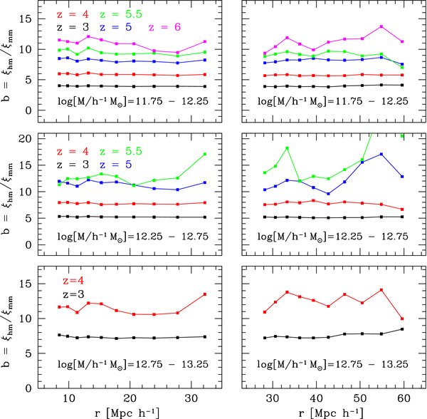
Figure 14. Halo bias as a function of scale. Right panels: the ratio ξhm/ξmm at large scales for different halo masses and redshifts, as labeled. Left panels: the same ratio at smaller separations that encompass the scales where AGN clustering has being measured by S07. At smaller separations, there is not significant scale dependence while the scatter of the measurement is lower than for large separations. The measured bias is higher by 2%–3% in the left hand panels, but this difference is within the scatter.
Download figure:
Standard image High-resolution imageIn order to overcome the shot noise due to the low abundance of rare halos, we decided to measure the bias from cross correlating the halo distribution to that of the dark matter. This allowed us to extend the measurements to cases where the halo–halo correlation is too noisy to define a meaningful bias. In Table 1, we report the bias results for  (top table) and for ξhm/ξmm (bottom table). In both cases, we measured at scales in the range 8 h−1 Mpc ⩽ r ⩽ 38 h−1 Mpc. The reported error corresponds to the variance among different bins (which might be taken as a rough representation of the true error of the measurement with the caveat that different bins are correlated). We find consistent results for the values of the bias derived from the two methods in those bins of mass and redshift where a reliable estimate can be obtained.
Table 1. Halo Bias Obtained from  (Top Table) or b = ξhm/ξmm (Bottom Table)
| log(M/M☉) = | 11.75 − 12.25 | 12.25 − 12.75 | 12.75–13.25 |
| z = 3 | b = 3.95 ± 0.07 | b = 5.3 ± 0.17 | b = 7.8 ± 0.69 |
| z = 4 | b = 5.97 ± 0.22 | b = 8.1 ± 0.57 | |
| z = 5 | b = 8.44 ± 0.61 | b = 11.6 ± 2.78 | |
| z = 5.5 | b = 10.1 ± 1.1 | ||
| z = 6 | b = 12.3 ± 1.6 | ||
| log(M/M☉) = | 11.75 − 12.25 | 12.25 − 12.75 | 12.75–13.25 |
| z = 3 | b = 3.97 ± 0.06 | b = 5.27 ± 0.09 | b = 7.38 ± 0.2 |
| z = 4 | b = 5.9 ± 0.13 | b = 7.88 ± 0.22 | b = 11.52 ± 0.54 |
| z = 5 | b = 8.25 ± 0.27 | b = 11.44 ± 0.5 | |
| z = 5.5 | b = 9.53 ± 0.39 | b = 12.78 ± 1.4 | |
| z = 6 | b = 10.96 ± 0.69 |
Notes. The values are consistent with each other within the bin-to-bin scatter, which is reported as the corresponding error.
Download table as: ASCIITypeset image
Finally, we compare our results to those of S07, who obtained the halo bias from  with,
with,
where rmin = 5 h−1 Mpc and rmax = 20 h−1Mpc. Using all halos more massive than Mmin = 2 × 10¹² h−1 M☉, S07 find beff(z = 3) = 6.2 and beff(z = 4) = 10.2 (respectively 17% and 5% lower than Jing's 1998 prediction). Using a similar mass cut to S07 and measuring the bias in the same way (i.e., from ξ20) we obtain beff(z = 3) = 6.07 and beff(z = 4) = 9.35 (where we have included a 6% correction due to the difference in the assumed cosmology). These values are in good agreement (within 8%). However, and contrary to S07, we have chosen Sheth et al. (2001) expression as our primary bias prediction for reasons already outlined in Section 2.2.
APPENDIX B: THE CONTRIBUTION OF BH MERGERS TO MASS ACCRETION
In this Appendix, we compute the expected contribution from mergers to the overall mass growth of the central black hole (BH) of a halo with mass M0 ∼ (1–2) × 1013 M☉ at z ∼ 3–4, typical of the z > 3 quasar hosts studied in this paper.
We trace the average mass growth history M(z) of a such halos at any redshift z by imposing the number density conservation within a comoving volume

The result is shown with a long dashed line in the left panel of Figure 15, which shows that such halos grow, on average, by about a factor of ∼6 within the redshift range 3 ⩽ z ⩽ 6.
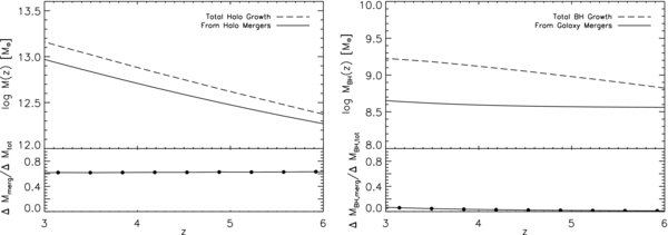
Figure 15. Left: growth history of halos with final mass ∼(1–2) × 1013 M☉, as derived from the halo mass function (long dashed line), compared to the growth history as predicted by integrating the merger rates of halos with progenitors mass ratios in the range 0.1 < ξ < 1 (solid line). Right: the long dashed line shows the total growth in the central black hole (BH) as derived from the long dashed line in the left panel and using Equation (5); the solid line is instead the BH growth derived by integrating the central galaxy merger rates. The dot-dashed line in the lower panel corresponds to BH growth when no delay is considered. Mergers contribute by only ≲7% to the overall growth of the central BH, at the most, if the delay due to dynamical friction is taken into account. See the text for details.
Download figure:
Standard image High-resolution imageWe then compute the expected growth of such halos due to halo and subhalo mergers. To such purpose, we estimate the average number of mergers per unit redshift dN/dz experienced by a given halo of mass M(z) at redshift z by integrating the halo merger rates
with ξmin = 0.1 and ξmax = 1. We take the halo merger rates per unit halo B[M(z), ξ, z]/n[M(z), z] from Fakhouri & Ma (2008), given as empirical fits to the Millennium Simulation, with n[M(z), z] the number density of halos of mass M(z) at redshift z. The quantity B[M(z), ξ, z] is the instantaneous merger rate at redshift z of halos with mass M(z) in units of h4 Mpc−3 dz−1 dξ−1 M−1☉, with ξ = M1/M2 the mass ratio between the masses of the progenitor merging halos with total mass M(z) = M1 + M2. The total mass accreted ΔM(z) on the halo of mass M(z) at each timestep Δz during the evolution is then
with ξ/(1 + ξ)M(z) the mass of the (smaller) merging halo. The solid line in the left panel of Figure 15 is the total mass accreted in mergers. As clear from the bottom panel, which shows the ratio between the cumulative mass grown by mergers and the total one derived from Equation (B1), mergers with 0.1 < ξ < 1 can account for most (∼65%) of the average growth of halos.8
It is then natural to ask how much of the central BH mass is actually contributed by mergers. The long dashed line in the upper right panel of Figure 15 shows the total growth of the central BH derived by assuming that at each z the BH has, on average, a mass as given by Equation (5). In order to estimate the contribution of BH mergers we, however, cannot naively use Equation (B3). We need to in fact take into account that when the smaller halo enters the virial radius of the larger halo, it takes about a dynamical friction timescale to sink to the center allowing for the central galaxies (and their BHs) to actually merge.
We therefore follow Shen (2009), and compute the central galaxy merger rates as ![$B_{\rm gal}[M(z),\xi,z]=B[M(z),\xi,z_e]\frac{dz_e}{dz}$](https://content.cld.iop.org/journals/0004-637X/718/1/231/revision1/apj297014ieqn16.gif) , being z the redshift of the actual merger with the central galaxy and ze the redshift at which the smaller halo first entered the virial radius of the larger halo. We use the Shen (2009) analytical fit to the function ze(z, ξ), which reproduces the Jiang et al. (2008) merger timescales well in the range 0.1 ⩽ ξ ⩽ 1. Adopting the results by Jiang et al. (2008) is particularly meaningful for this paper. Their subhalo merger timescales were in fact derived for a suite of high-resolution numerical simulations performed on halos with masses M > 5 × 10¹² h−1 M☉, in the range of interest for our paper, and with a virial mass definition equal to that used in this paper (see Section 2). The study by Boylan-Kolchin et al. (2008), for example, yields somewhat different merging timescales with respect to those found by Jiang et al. (2008; see also Shen 2009). However, their results were based on parent halos about an order of magnitude less massive than the ones of interest here, and with a significantly different definition of virial mass.
, being z the redshift of the actual merger with the central galaxy and ze the redshift at which the smaller halo first entered the virial radius of the larger halo. We use the Shen (2009) analytical fit to the function ze(z, ξ), which reproduces the Jiang et al. (2008) merger timescales well in the range 0.1 ⩽ ξ ⩽ 1. Adopting the results by Jiang et al. (2008) is particularly meaningful for this paper. Their subhalo merger timescales were in fact derived for a suite of high-resolution numerical simulations performed on halos with masses M > 5 × 10¹² h−1 M☉, in the range of interest for our paper, and with a virial mass definition equal to that used in this paper (see Section 2). The study by Boylan-Kolchin et al. (2008), for example, yields somewhat different merging timescales with respect to those found by Jiang et al. (2008; see also Shen 2009). However, their results were based on parent halos about an order of magnitude less massive than the ones of interest here, and with a significantly different definition of virial mass.
The solid line in the upper right panel of Figure 15 shows the total mass accreted onto the central BH via mergers. It is clear that subhalo mergers are not the dominant source of growth for massive BHs at high redshift, as also independently found by several other groups (e.g., Volonteri et al. 2005). The cumulative fraction of BH mass at z = 3 grown via mergers is only ∼7%, reducing to just a few percent at 4 < z < 4.5 where most of the tightest constraints from clustering come from (see Section 3). Adopting the Boylan-Kolchin et al. (2008) merging timescales would increase the contribution from mergers by just a factor of ≲2. Note, also, that our estimate is actually an upper limit. In fact, this calculation assumes that all of the incoming dark matter substructures actually contain a BH as massive as what is predicted from Equation (5) that efficiently merges with the central BH. Moreover, we have not considered that the delay time for BH mergers is even longer than those of galaxies (see, e.g., Merritt & Milosavljevic 2005 for a review), a correction which would further drop the contribution of BH mergers.
In the lower right panel of Figure 15, we also show the predictions of the same model when no delay is considered between halos and central BH mergers. In this model, satellite BHs instantly merge with the central BH of the parent halo just after the merging of their host halos. Although this assumption is obviously too simplistic, as it neglects any dynamical friction time delay, it can be safely regarded as a secure upper limit to the contribution of mergers to the overall BH growth. As shown in the right panel of Figure 15, in this extreme model the growth of BH mass via mergers is comparable to that via accretion, accounting for about 50%–60% of the final BH at z ∼ 3.
From the study undertaken in this section, we conclude that, in the physically plausible case that a significant dynamical friction time- delay is present between host halo and central BH mergers, it is a good approximation to neglect BH growth via mergers in the continuity equation model discussed in Section 2. However, the same is not true for quasar activations. The model discussed in Section 2 holds in reproducing both the quasar luminosity function and quasar clustering only in the hypothesis that BH growth via accretion parallels that of the host dark matter halo with no time delay between the two. The latter assumption was also adopted by several other groups to boost and thus facilitate the match to the high-z, luminous quasar number counts (e.g., Wyithe & Loeb 2003; Scannapieco & Oh 2004; Lapi et al. 2006; Shen 2009).
For completeness, however, we present in the next section the results of a fully self-consistent model that evolves the BH mass function through a continuity equation with accretion and mergers, with no delay in any of its components. We will discuss how the outcome of such a model strengthens our general conclusions.
APPENDIX C: MODELS WITH ACCRETION PLUS MERGERS
Inserting mergers in the continuity equation of Equation (10) implies a format of the type
where
and
are, respectively, the merger rate of incoming smaller mass BHs with mass M'BH = MBHξ/(1 + ξ) and M''BH = MBH/(1 + ξ) that merge into a BH of final mass MBH, and the merger rate of BHs with initial mass MBH that merge into more massive BHs of mass M'BH = MBH(1 + ξ)/ξ and M''BH = MBH(1 + ξ) (in both Equations (C2) and (C3) we set ξmin = 0.1, and add the factor of 1/2 to avoid double counting).
If we assume that no delay is present between the mergers of the BHs and their parent halos, the probability of BH mergers per unit time is simply given by the halo merger rate adopted above, i.e.,
By simply knowing, at each timestep, the mapping between infalling halo mass and its central BH (given by Equation (5)), we can then compute the expected average rate for any BH merger event. By further assuming the AGN luminosity function to be known from observations (we here adopt the analytical derivation by SWM), we can simply integrate the right-hand side of Equation (C1) and derive the BH function at all redshifts.
The result is shown in Figure 16, the left panel of which shows the integrated BH mass density ρ(MBH > 108 M☉, z), in the mass and redshift range of interest here, for the reference model (λ = 0.25, α = 1, = 0.15) with no mergers (long dashed lines), and with mergers (solid lines), as labeled, while the right panel compares the resulting BH mass functions for the two models at three different redshifts, from bottom to top, z = 6, 4, and3. The two filled circles in the left panel mark the expected BH mass density at z = 3 and z = 4 expected from Equation (20), adopting a duty cycle of P0 = 0.25 and P0 = 0.5, respectively, for a model consistent with the measured quasar clustering (see Figure 12). As above, we here neglect any source of scatter in the relation between luminosity and halo mass to maximize the predicted clustering for a given model. We find that, irrespective of the differences in the AGN luminosity function adopted here and in the main text, the results for the pure accretion model match those presented in Figure 12. When mergers are included, the estimated BH mass density above 108 M☉ is larger by a factor of ≳2, than the one from accretion alone. We should emphasize that we consider this factor of 2 to be an extreme upper limit on the impact of mergers, since it ignores even the effects of dynamical friction delay, which we have shown in the previous Appendix to drastically reduce the BH merger growth. More importantly, however, any growth of the BH mass function via mergers exacerbates the tension we have highlighted between high-redshift quasar clustering and the luminosity function. Mergers add mass to the BH population without associated luminosity, so reproducing the observed luminosity function with the BH population implied by the BH–halo relation requires a still higher radiative efficiency.
Figure 16. Left: accreted black hole (BH) mass density above log MBH/M☉ > 8 as a function of redshift, for the reference model characterized by λ = 0.25 and = 0.15, with no mergers (long dashed line), and with mergers (solid line); the solid, filled circles are the z = 3 and z = 4 BH mass density obtained via Equation (20) by assuming a duty cycle of P0 = 0.25 and P0 = 0.5, respectively, as in the reference model (Figures 8 and 12). Right: comparison between the resulting BH mass functions for the no-merger (long dashed) and merger (solid) models, at three different redshifts, from bottom to top, z = 6, 4, and3.
Download figure:
Standard image High-resolution image
Footnotes
- 5
S07 in their clustering analysis remove the "bad" fields, i.e., those which do not fully satisfy their photometric criteria of completeness, but also report clustering measurements performed on the whole sample. We presume throughout this paper that the "good" measurements (shown with diamonds) are more reliable and the ones that any successful model must reproduce; however, following S07, we will always report both sets of data in the figures. The smaller number of pairs at small separations in the "good" sample could lead to systematic errors in the correlation length estimate as well as larger statistical uncertainties (Y. Shen 2008, private communication).
- 6
We also insert a Jacobian correction factor in their Equation (4) between observed B-band and bolometric luminosities.
- 7
- 8
We note here that the exact value of the adopted ξmin does not alter our overall conclusions. For example, setting ξmin = 0.01, increases the growth of the parent halo via mergers to 90%–95%, but it has a negligible impact on the mass growth of the central BH.