


ABSTRACT
We address the origin of the enhancement of ∼40 keV to 5 MeV ions at the solar wind termination shock. Using self-consistent two-dimensional hybrid simulations (kinetic proton, fluid electron) of a shock moving through a plasma similar to that observed in the outer heliosphere, we conclude that the observed ion enhancements are consistent with accelerated "core" interstellar pickup ions (those that have not previously undergone any significant energization) by the termination shock via a combination of shock drift acceleration and particle scattering in meandering magnetic fields in the vicinity of the shock. In addition to the consequences for our understanding of anomalous cosmic rays, this work is also relevant to the more-general long-standing problem of accelerating low-energy particles by shocks that move nearly normal to a mean magnetic field.
Export citation and abstract BibTeX RIS
1. INTRODUCTION
When Voyagers 1 and 2 each crossed the termination shock, large enhancements of ∼40 keV to 5 MeV ions were observed to peak at the time of the shock crossing (Decker et al. 2005, 2008) suggesting strongly that it is the source of the accelerated particles. Low-energy anomalous cosmic rays (ACRs) were also seen in the solar wind before the shock crossings (Krimigis et al. 2003; McDonald et al. 2003) which were inferred to be coming from the shock (Stone et al. 2005; Decker et al. 2005; Giacalone & Jokipii 2006; Gloeckler & Fisk 2006). Recently it was shown that there may even be sufficient energy density in these particles to account for the observed slowing of the solar wind prior to the Voyager 2 shock crossing (Florinski et al. 2009; Richardson et al. 2008). In contrast to the low-energy ACRs, the fluxes of the highest-energy ACRs continued to rise after the crossing of the shock (Stone et al. 2008), suggesting that the source of these particles is somewhere other than where the Voyagers crossed it. There have been a number of interpretations of this (e.g., McComas & Schwadron 2006; Florinski & Zank 2006; Kota & Jokipii 2008; Jokipii & Kota 2008; Schwadron et al. 2008; Fisk & Gloeckler 2009), but it remains without a well-accepted explanation.
A number of authors have addressed the acceleration of low-energy charged particles at the termination shock. A key issue addressed in these studies is the general problem of accelerating low-energy particles that are not well described by diffusive shock acceleration theory. This is known as the injection problem. Kucharek & Scholer (1995) used one-dimensional hybrid simulations of pickup ions interacting with oblique shocks (see also Liewer et al. 1995) to show that injection is generally not a problem for quasi-parallel shocks. They argued that the termination shock is locally quasi-parallel on enough occasions (due to turbulence) to account for the observed ACR fluxes when extrapolating their results to high energies. Giacalone (2005) explicitly included the effect of large-scale magnetic turbulence, superimposed on an average magnetic field perpendicular to the shock normal, to show that even thermal solar-wind ions are accelerated by the shock. Ellison et al. (1999) used a Monte Carlo numerical calculation of pickup-ion acceleration using an assumed phenomenological scattering rate and also showed that injection is not a problem. Other ideas have also been discussed, including so-called "surfing" acceleration (Zank et al. 1996a, Lee et al. 1996, le Roux et al. 2000). Alternatives to accelerating low-energy particles directly by the shock have also been discussed (e.g., Giacalone et al. 1997; Fisk et al. 2006).
In this study, we perform simulations of the solar wind, magnetic field, and particle distributions in the vicinity of the termination shock at the time Voyager 2 crossed it. We examine the distributions of three different proton populations: (1) thermal solar wind, (2) freshly ionized interstellar pickup ions, and (3) a pre-existing population of energetic particles. This study is similar to our previous one (Giacalone 2005) except that here we use initial values for physical parameters based on Voyager 2 observations. In addition, we include the effects of two particle species (2 and 3) that were neglected in the previous study. Our results are directly compared to Voyager 2 Low Energy Charged Particle (LECP) observations to interpret the enhancement of ∼40 keV to 5 MeV ions as it crossed the termination shock in 2007.
2. NUMERICAL SIMULATION MODEL
For this study, we use the well-known hybrid simulation in which ions are treated kinetically and the electrons as a charge-neutralizing, massless fluid (cf. Winske & Omidi 1996). This model has seen wide use for nearly 30 years for studies of space plasmas and shocks in particular (e.g., Leroy et al. 1981; Goodrich 1985; Winske & Omidi 1996, and references therein). It is useful for our study because it includes the basic physics of shock microstructure occurring on ion length and timescales. Since the particles of interest in this study range from thermal solar wind up to about 100 keV, it is important to self-consistently treat the ion-kinetic physics, including their effect on the electric and magnetic fields in the vicinity of the shock. This permits a detailed examination of the heating of the incident protons and the acceleration of a fraction of them to high energies, which is the purpose of the present study.
The particular model we use for this study is very similar to that of Giacalone (2005). The main difference is that in this study, two other proton populations, in addition to thermal solar wind protons, are considered: freshly ionized interstellar protons and a population of high-energy particles constituting a suprathermal tail on the incident distribution. All three populations contribute to the self-consistent simulations, but we keep track of each species separately for diagnostic purposes. In addition, we use input values that are based on Voyager 2 observations made at the time of one of the termination shock crossings in 2007.
In our calculation, physical quantities are defined on a two-dimensional Cartesian grid of dimensions 500 c/ωp,1 × 4000 c/ωp,1 (where c is the speed of light and ωp,1 is the total proton plasma frequency in the ambient solar wind upstream of the shock). Plasma initially flows in the positive x-direction (the shorter of the two spatial dimensions) where it reflects off of a rigid boundary resulting in a shock that moves back into the flow. The average magnetic field lies in the z-direction (the longer of the two dimensions). Superimposed on both the field and flow vectors at the start of the simulation (and injected continuously with the incoming solar wind at the left boundary, as in Figure 2 below) are random components representing pre-existing turbulence in the solar wind. This is generated by summing many individual circularly polarized Alfvén waves with a given wave number and frequency, and an amplitude derived from an assumed power spectrum with a variance σ21, coherence scale Lc, and power-law spectral index −5/3. The minimum wavelength is set equal to 10c/ωp,1 and the maximum wavelength is equal to the box dimension in the z-direction. See Giacalone (2005) for additional details. At late times in our simulation, the shock is rippled in response to large-scale turbulence, which is a combination of the remnant initial fluctuations, that injected at the left boundary, and that which evolves self-consistently from the simulation. This is a reasonable representation of the solar wind, interplanetary magnetic field, and termination shock in the outer heliosphere over small fractions of an AU in scale, but still many times larger than the gyroradii of the particles of interest in this study. We note that the gyroradius of a 1 MeV proton in the assumed upstream magnetic field (see Table 1) is about xmax, the size of the simulation domain in the x-direction, and about 8 times smaller than zmax. Thus, our simulations are only applicable to protons with energies less than ∼1 MeV and are well suited for those with energies below about 100 keV (note also that because the field is compressed downstream of the shock, the gyroradius is reduced in this region).
Table 1. Simulation Parameters
| Parameters | Values |
|---|---|
| nsw,1 | 0.001 cm−3 |
| V1 | 3.2 × 107 cm s−1 |
| npu,1 | 3.33 × 10⁻⁴ cm−3 |
| nep,1 | 1.2 × 10⁻⁷ cm−3 |
| np,1 | 1.33 × 10⁻³ cm−3 |
| B1 | 0.05 nT |
| ωp,1 | 48.1 s-1 |
| Ωp,1 | 4.79 × 10⁻³ s-1 |
| VA,1 | 3.0 × 106 cm s−1 |
| Tsw,1 | 104 K |
| βsw,1 | 0.139 |
| βe,1 | 0.139 |
| MA,1 | 10.6 |
| σ21 | 1.25 × 10⁻³ nT2, 5 × 10⁻⁴ nT2 |
| Lc | 0.17 AU |
Notes. The subscript sw refers to solar wind, pu for pickup ions, ep for energetic particles, p is for all protons, e is for electrons, and 1 refers to the region upstream of the shock. The last two rows are the turbulence variance (two values are considered) and coherence length. The other symbols in this table are standard plasma-physics notation.
Download table as: ASCIITypeset image
The initial conditions of the plasma and fields are based on Voyager 2 observations made during the period of time when it crossed the termination shock (Richardson et al. 2008; Burlaga et al. 2008; Decker et al. 2008). The parameters we use are given in Table 1. The included pickup ions are assumed to be freshly ionized with a number density that is 25% of the total, which is roughly consistent with Table 1 of Fisk et al. (2006). In addition, we also include a population of energetic particles with a distribution such that f ∝ w−5 (Fisk & Gloeckler 2006), where f is the phase-space distribution function and w is the particle speed in the plasma frame. Note that for the parameters given in Table 1, our assumed simulation domain corresponds to a region of 0.021 AU × 0.17 AU. The simulation proceeds forward in time from t = 0 to t = 100 Ω−1p,1 = 5.8 hr, where Ωp,1 is the proton cyclotron frequency in the mean upstream magnetic field. We assume a grid-cell size of Δx = Δz = 0.5c/ωp,1, a time step of Δt = 0.01 Ω−1p,1, and an anomalous resistivity of η = 1 × 10−44πω−1p,1. The particles are initially uniformly distributed in the computation domain using 30 particles per grid cell (combined solar wind protons, pickup protons, and energetic particles). The electrons are treated adiabatically. Their pressure is related to their density (the same as the total proton density) by Pe ∝ n5/3e. It is also important to note that because of the presence of an ignorable coordinate (y) in our simulation, protons are not able to move off of individual magnetic field lines (e.g., Jokipii et al. 1993). They do, however, move normal to the mean magnetic field because they follow along field lines that meander in space. This field-line random walk has been shown to be the dominant contribution to cross-field transport of low-energy particles (Giacalone & Jokipii 1999).
Figure 1 shows the differential intensity, dJ/dE, measured in the shock rest frame as a function of kinetic energy, E, for the three different proton populations used in our simulation. The dashed curve (a) is the thermal solar wind. It is assumed to be Maxwellian in a frame moving with the upstream bulk flow speed Vsw,1 with a temperature Tsw,1 (see Table 1). The thermal, or root-mean-square speed of the particles measured in a frame co-moving with the bulk flow speed in any given direction is related to the temperature by (1/2)mv2th,sw,1 = kTsw,1, where m is the proton mass, and k is the Boltzman constant. The solid curve (b) is the freshly ionized pickup ions (which we also refer to as "core" pickup ions) with a number density taken to be 25% of the total number density. There is a sharp drop in the distribution at twice the solar-wind speed corresponding to an energy of about 2 keV. The dot-dashed curve (c) represents a quiet-time tail of energetic particles assumed to be accelerated elsewhere in the heliosphere as discussed above. Note that it has a power-law dependence on energy such that dJ/dE ∝ E−1.5 (e.g., Fisk & Gloeckler 2006). In order to determine their normalization relative to the solar wind and core pickup ions, we use the Voyager 2 LECP observations of energetic ions seen prior to the termination shock crossing (d and e, in Figure 1). These have been interpreted as particles coming from the termination shock. The data shown in Figure 1 are taken during 2007 prior to the Voyager 2 shock crossings, which took place from DOY 242–244. The open squares represent averages from DOY 007–085 and the solid circles are averages from DOY 085–163, presumably when Voyager 2 was closer to the shock. We assume that the high-energy, quiet-time, tail that exists in the solar wind distribution must be at an intensity that is lower than that of the particles seen upstream of the termination shock. Thus, the intensity of these particles assumed in our study can be considered as an upper bound to the actual intensity of these particles.
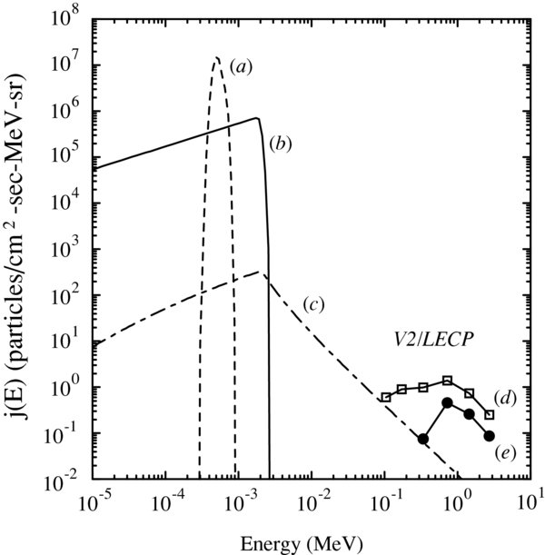
Figure 1. Differential intensity vs. kinetic energy in the shock-rest frame for the three proton populations at the start of the simulation and continuously injected with the solar wind at the left simulation boundary. Population a (dashed curve) are thermal solar wind protons, b (solid curve) are freshly ionized pickup ions, and c (dot-dashed curve) are a high-energy tail whose intensity is adjusted to be just below the Voyager 2 observations of termination shock particles seen upstream of the shock in the solar wind (symbols). The open squares represent averages from 07/007–07/085 and the solid circle symbols are from 07/085–07/163.
Download figure:
Standard image High-resolution image3. RESULTS AND DISCUSSION
Figure 2 shows a two-dimensional color-coded representation of the magnetic-field strength (left) and density of particles with energies greater than 5 keV (right) at the end of one of our simulations (the one with σ21 = 1.25 × 10⁻³ nT2). The plot of the field strength reveals the rippling of the shock surface in response to its interaction with upstream turbulence. In the plot of the density all protons with energies greater than 5 keV, the shock position is indicated as a black curve, and the white curves are magnetic field lines. The density of these protons is not uniform along the shock. This was also seen in our previous study (Giacalone 2005) and was attributed to the variation in acceleration efficiency at different portions along the shock, depending on the local geometry of the magnetic field and shock. When the magnetic field is locally oblique to the shock-normal direction, particles are more-easily reflected back upstream of the shock compared to situations in which the field is nearly normal to the shock. Because turbulent fluctuations exist on scales much larger than the particle gyroradii, local-geometry variations such as these are expected to exist along the shock front leading to intensity variations of low-energy ACRs.
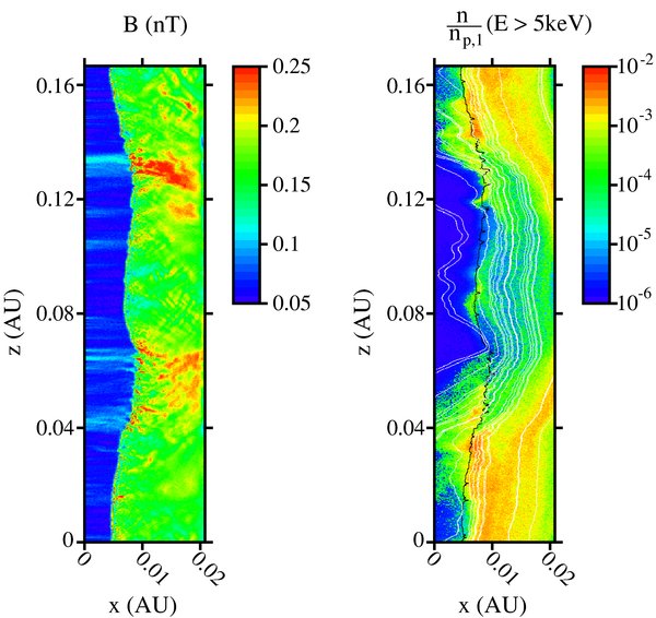
Figure 2. Color-coded representations of the magnetic field strength (left) and number density normalized to the total upstream proton density (on a logarithmic scale) of all protons with energies greater than 5 keV (right) over the entire domain of one of the simulations of the termination shock at the end of the simulation (t = 100 Ω−1p,1 = 5.8 hr). The legends to the right of each plot indicate the values that the colors refer to. In the right plot, the shock front location is shown as a black line, and several magnetic lines of force are shown as white lines. The flow of the solar wind plasma is from left to right in these plots.
Download figure:
Standard image High-resolution imageFigure 3 shows the trajectory of a core pickup ion accelerated to high energies. The right plot shows the particle kinetic energy as a function of time. The left two plots show the particle z location (top) and kinetic energy (bottom) as functions of the x position relative to the average shock-rest frame. Because the shock surface is rippled and also moves back and forth in time, the instantaneous shock location cannot easily be represented on this plot. Instead, we indicate the maximum and minimum extent of the shock surface relative to an average position as a gray-shaded band in these plots. This particle, like all those we have examined, gains its energy at the shock. The energy comes from drifting (due to the both the gradient of the field strength and curvature of field lines in the shock layer) in the direction of the local electric field. This is essentially what is expected from shock-drift acceleration.
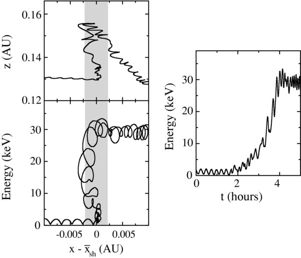
Figure 3. Various representations of the trajectory of an accelerated core pickup ion. Lower left: particle kinetic energy vs. the x position measured relative to an average shock location  . Upper left: the particle's z location vs.
  . The gray-shaded band in these two plots represent the maximum and minimum extent of the shock front relative to the average (note that the instantaneous location of the shock is a function of z and time). Right: particle kinetic energy as a function of time.
Download figure:
Standard image High-resolution imageFigure 4 shows the differential intensity as a function of kinetic energy computed at the end of the simulation. It is in the same format as Figure 1, except that the simulation results for each proton population are compared with Voyager 2 observations in the heliosheath, downstream of the shock. The simulated spectra were computed over the spatial region 220c/ωp,1 < x < 500c/ωp,1 and 0 < z < 4000c/ωp,1, which is essentially the entire downstream region. This averaging is done to remove the variations shown in the right of Figure 2. The symbols with error bars are Voyager 2 LECP measurements taken after the termination shock had been crossed in 2007 from DOY 241–319.
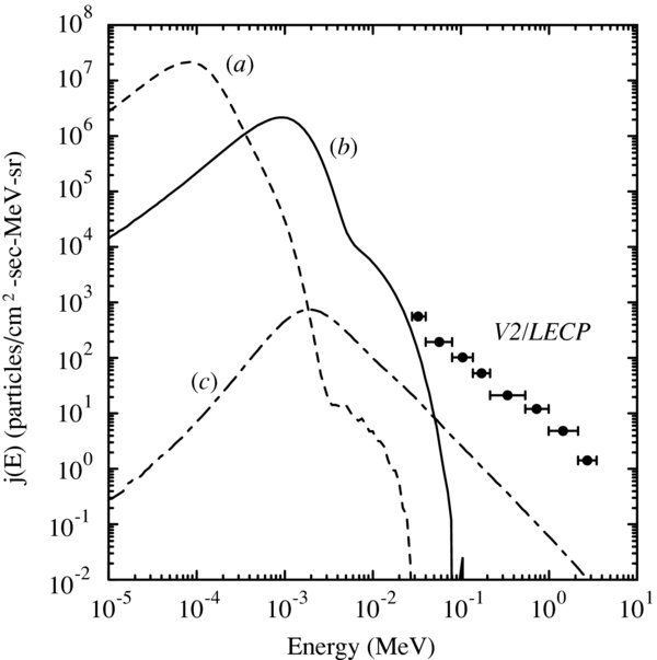
Figure 4. Differential intensity vs. kinetic energy for protons measured in the region downstream of the shock at the end of the simulation t = 100 Ω−1p,1 = 5.8 hr. The format is the same as Figure 1 except that the symbols are for Voyager 2 LECP observations averaged over a different time interval (07/241–07/319). The spatial region over which the simulated proton distributions are computed is 220c/ωp,1 < x < 500c/ωp,1 and 0 < z < 4000c/ωp,1.
Download figure:
Standard image High-resolution imageComparison of the simulated energy spectra with the Voyager 2 LECP observations suggests that low-energy ACRs are accelerated core interstellar pickup ions. The shoulder in the distribution of core pickup ions (labeled b in Figure 4) extending from ∼6–60 keV nearly matches the intensity of observed ions (with Z > 1, where z is the charge normalized to the proton charge). We also conclude that the Voyager 2 observations are not consistent with the compression of the pre-existing high-energy tail on the upstream distribution (Fisk et al. 2006) since the simulated intensity of the population labeled c in Figure 4 is about 2 orders of magnitude lower than the Voyager 2 LECP observations. It is also noteworthy that some solar wind protons are accelerated to high energies as well (as seen in the shoulder in the curve labeled a), but their intensity is far too low to account for the Voyager 2 LECP observations.
Because our simulations are run for a relatively short time, the simulated energy spectrum falls off rapidly at high energies. In addition, the maximum energy is also limited by the finite size of the simulation domain. It is instructive to estimate the maximum energy for the assumed simulation time based on the diffusive shock acceleration theory (ignoring losses imposed by the finite system size). The acceleration time, τA, in non-relativistic form, is given by (e.g., Forman & Drury 1983; Drury 1983)
where the subscripts 1 and 2 refer to the upstream and downstream regions of the shock, respectively, κxx is the particle diffusion coefficient in the direction normal to the shock and V is the flow speed, in the shock frame of reference.
A reasonable assumption for our purposes is that the diffusion coefficient downstream of the shock is related to that upstream by κxx,2 = κxx,1/r2, where r = V1/V2 is the density compression ratio. This assumes the diffusion coefficient is related to the variance in the magnetic field whose components transverse to the shock normal are compressed by a factor of r (the variance is increased by r2). For our case, the shock moves normal to the mean magnetic field so the appropriate diffusion coefficient is that normal to the field. We further assume that the perpendicular diffusion coefficient is a constant times the parallel diffusion coefficient, i.e., κ⊥ =  κ∥ with typically of the order of 0.01 (e.g., Giacalone & Jokipii 1999). We use quasi-linear theory to estimate the parallel diffusion coefficient. Equation (B4) of Giacalone & Jokipii (1999) gives an expression for κ∥ based on the same form of the turbulence power spectrum used here.3 Using these assumptions, it is readily shown that the acceleration time is given by
where we have assumed both w ≫ w0 and w ≪ Ωp,1Lc to derive this result. To estimate the maximum energy for the given simulation time, we solve this equation for w (to get the kinetic energy) for τA = 100 Ω−1p. We take = 0.01, r = 2.5, V1 = Vsw,1 and values from Table 1 and find w ≈ 1.4 × 108 cm s-1, corresponding to an energy of about 10 keV. This is consistent with our simulation results. If the simulations were run longer, we predict that a higher maximum energy would be achieved. Also, it is interesting to note that based on these parameters the time to accelerate protons to 50 keV is about 17 hr.
To examine the time dependence of the high-energy portion of the core pickup-ion distribution in our simulation, we show in Figure 5 energy spectra at three different times. Clearly, the tail is continuing to evolve as time increases. The dashed line in this figure is a simple power-law fit to the steady part of the shoulder. It has a spectral index of −1.6, which is consistent with the prediction of diffusive shock acceleration for a shock with compression ratio r = 2.4, which is similar to what we find in our simulations.
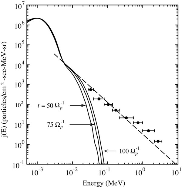
Figure 5. Energy spectra downstream of the shock for core pickup ions (solid lines in Figures 1 and 4) at three different times, as indicated. In all cases, the distribution is averaged over all z. For the plot at t = 75 Ω−1p,1, the distribution is computed over the region 290c/ωp,1 < x < 500c/ωp,1, and for t = 50 Ω−1p,1, it is 355c/ωp,1 < x < 500ωp,1.
Download figure:
Standard image High-resolution imageWe expect that if the simulations could be made to be much bigger and run for much longer than we are currently capable, the tail would continue to fill in at high energies, and, presumably, would match the Voyager 2 observations. Therefore, a reasonable interpretation of our simulations and the direct comparison with Voyager 2 LECP observations strongly suggest that low-energy ACRs, observed to be enhanced at the termination shock, are accelerated core pickup ions.
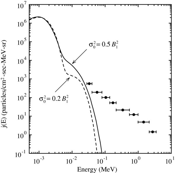
In Figure 6, we show the core-pickup-ion energy spectra for two simulations with different values of the input magnetic-field variance. As the variance is reduced, the overall acceleration efficiency is also reduced, but the resulting spectra still nearly match up to the low-energy end of the Voyager 2 LECP data. The reason the injection efficiency is lower is that weaker turbulence results in less field-line meandering, leading to fewer favorable locations along the shock for reflection and acceleration of freshly ionized pickup ions. In the limit of no fluctuations, there is no field-line random walk, and the local magnetic field is normal to the shock everywhere, which is not favorable for acceleration. We do not think that this is realistic for the termination shock since the variance is known to be a significant fraction of the energy in the mean field (Burlaga et al. 2007). Moreover, the coherence scale of interplanetary magnetic turbulence, which is related to the scale of field-line meandering, in the distant solar wind is likely much larger than we have simulated (Zank et al. 1996b). We expect that there is sufficient interplanetary turbulence at large scales to give rise to effects similar to that which we have simulated.
Figure 6. Downstream energy spectra of core pickup ions at the end of two simulations with different values of the input magnetic variance, as indicated.
Download figure:
Standard image High-resolution image
As a final comment, the results from our simulations are also generally consistent with other observations made by Voyager 2 as it crossed the termination shock. For example, the simulated downstream sound speed based solely on solar-wind protons only (the sound speed of population a in Figures 1 and 3) is less than the downstream flow speed. This is consistent with the results reported by Richardson et al. (2008) whose instrument does not measure pickup ions. We note that the sound speed of the entire plasma, including pickup ions and the negligible contribution of the pre-existing high-energy tail particles, is greater than the downstream flow speed, as required for a shock. In addition to this, we also find that the basic foot-ramp-overshoot microstructure of the shock (e.g., Winske 1985) is only seen at some places along the shock and not others. This is due to the interaction with the upstream turbulence leading to a spatially and temporally dependent shock profile. This is also consistent with the observations in which Voyager 2 crossed the shock at least 5 times, but only on one occasion was this simple foot-ramp-overshoot profile observed (Burlaga et al. 2008).
4. SUMMARY
We simulated a small portion of the termination shock using a two-dimensional hybrid-plasma model (kinetic protons, fluid electrons) to interpret the origin of the enhancement of ∼40 keV to 5 MeV ions seen by Voyager 2 LECP as the spacecraft crossed the shock (Decker et al. 2008). We used plasma and field parameters consistent with those measured by Voyager 2 (Richardson et al. 2008; Burlaga et al. 2008). We separated the total proton distribution into three components to examine the relative contribution of each. One component was thermal solar wind protons, a second was freshly ionized ("core") interstellar pickup ions, and the third was a pre-existing high-energy tail. We find that the acceleration of the second population, core pickup ions, at the shock best explains the low-energy ion enhancements seen by Voyager 2 LECP. The simulated distribution of core pickup ions downstream of the shock nearly matches that at the lowest energy observed. Higher energies in our model are not possible because of the limitations imposed by the small computation domain that we used. The simulations presented in our study are generally applicable for particles with energies less than a few hundred keV.
The mechanism by which core pickup ions are accelerated at the termination shock is similar to standard shock drift acceleration, except that the large-scale magnetic turbulence plays a critical role. It results in the spatial meandering of magnetic lines of force on scales that are much larger than the gyroradii of low-energy ACRs leading to variations in the local morphology of magnetic field lines and shock surface. At some places along the shock front, the local morphology is favorable for the direct reflection of a fraction of the incident pickup ions back upstream where they follow approximately along magnetic field lines that then intersect the shock elsewhere and the pickup ions gain more energy. This has, at least, two important effects: first, it leads to intensity variations in the low-energy accelerated pickup ions along the shock front. At higher energies, the intensity variations tend to be smoothed out because of the increased mobility of these particles. The second effect is that this is an efficient means of accelerating particles at a perpendicular (on average) shock, thereby overcoming the well-known problem of injection.
As a final note, in addition to the observed low-energy ion enhancements, both Voyagers observed significant enhancements of energetic electrons at the termination shock (Decker et al. 2008). Although our simulation treats the electrons as a fluid and does not explicitly describe their acceleration by a shock, the results of our calculation are relevant to this problem. As was first discussed by Jokipii & Giacalone (2007), electrons move rapidly along magnetic field lines which, for the case of a perpendicular shock, intersect the shock in several places. The resulting multiple shock encounters by fast-moving electrons chiefly along field lines will lead to efficient acceleration and may provide a qualitative explanation of the Voyager results.
This work was supported, in part, by NASA under grants NNX07AH19G, NNX09AG32G, and NNX07AB02G, and by NSF under grant ATM0447354.
Footnotes
- 3
It should be noted that there is a typographical error in Equation (B4) of Giacalone & Jokipii (1999). The quantity Ω20 appearing in the numerator of the first ratio after the equality, should, in fact, be in the denominator.