


ABSTRACT
Observational and modeling results indicate that typically the leading magnetic field of bipolar active regions (ARs) is often spatially more compact, while more dispersed and fragmented in following polarity. In this paper, we address the origin of this morphological asymmetry, which is not well understood. Although it may be assumed that, in an emerging Ω-shaped flux tube, those portions of the flux tube in which the magnetic field has a higher twist may maintain its coherence more readily, this has not been tested observationally. To assess this possibility, it is important to characterize the nature of the fragmentation and asymmetry in solar ARs and this provides the motivation for this paper. We separately calculate the distribution of the helicity flux injected in the leading and following polarities of 15 emerging bipolar ARs, using the Michelson Doppler Image 96 minute line-of-sight magnetograms and a local correlation tracking technique. We find from this statistical study that the leading (compact) polarity injects several times more helicity flux than the following (fragmented) one (typically 3–10 times). This result suggests that the leading polarity of the Ω-shaped flux tube possesses a much larger amount of twist than the following field prior to emergence. We argue that the helicity asymmetry between the leading and following magnetic field for the ARs studied here results in the observed magnetic field asymmetry of the two polarities due to an imbalance in the magnetic tension of the emerging flux tube. We suggest that the observed imbalance in the helicity distribution results from a difference in the speed of emergence between the leading and following legs of an inclined Ω-shaped flux tube. In addition, there is also the effect of magnetic flux imbalance between the two polarities with the fragmented following polarity displaying spatial fluctuation in both the magnitude and sign of helicity measured.
Export citation and abstract BibTeX RIS
1. INTRODUCTION
A bipolar active region (AR) is, in general, believed to be formed by an Ω-shaped flux tube rising through the photosphere, in which the magnetic filed is generated by some solar dynamo in the thin tachocline layer at the base of the solar convection zone. The two legs of the Ω-shaped flux tube form the two opposite polarities of the bipolar AR, one leading in the sense of solar rotation and the other following. Observations have shown a clear asymmetry in the morphology of the leading and the following polarities (see Bray & Loughhead 1979). The leading polarity of ARs generally lies closer to the equator than the following polarity giving the whole AR a tilt towards the solar equator, i.e., Joy's Law (Zirin 1988), which describes the statistical mean behavior of the AR tilts. In the 23rd solar cycle from 1996 to 2007, the leading (following) polarity in the northern hemisphere possesses positive (negative) magnetic field, with the magnetic field oppositely oriented in the southern hemisphere, i.e., the negative (positive) magnetic field in the leading (following) polarity. Such ARs follow the Hale polarity law (Hale et al. 1919). On the other hand, the magnetic flux of the leading polarity in such bipolar ARs tends to be concentrated in large well formed sunspots, whereas the flux of the following polarity tends to be less organized and more fragmented in appearance. The leading sunspots tend to be larger in area, fewer in number, and have a longer lifetimes than the following spots (see a review by Fan 2004, and references therein). The considerably more fragmentation observed in the following polarity is a well known property of mature, predominantly well defined bipolar ARs (see Zwaan 1981; Canfield 1999; Canfield & Russell 2007). These properties reflect the subsurface dynamical evolution of the emerging magnetic fields.
The origin of the observed morphological asymmetry is not clear and models of flux emergence are not yet sophisticated enough to handle the problem in detail. Fan et al. (1993) and Fan & Fisher (1996) found that an asymmetry in the magnetic field strength develops between the leading and following legs of emerging loops because the Coriolis force, and the tendency for the tube plasma to conserve angular momentum, drives a counter-rotational flow of plasma along the emerging loop, which gives rise to an effective asymmetric stretching of the two legs of the loop with a greater stretching, and hence a stronger field strength, in the leading leg (see a more detailed explanation in a review by Fan 2004). Fan & Fisher (1996) argued that the stronger field along the leading leg of the emerging loops makes it less subject to deformation by the turbulent convection and therefore explains the more coherent and less fragmented appearance of the leading polarity of an AR. An additional effect of the Coriolis force is to generate an asymmetry in the east–west inclination of the two sides of the loop (see Moreno-Insertis et al. 1994; Caligari et al. 1995, 1998). The emergence of such an eastward-inclined loop is expected to produce apparent asymmetric east–west proper motions of the two polarities of the emerging region, with a more rapid motion of the leading sunspot away from the emerging region compared to the motion of the following sunspots. This has been observed in young ARs and sunspot groups (see Chou & Wang 1987; van Driel-Gesztelyi & Petrovay 1990; Petrovay et al. 1990).
Our purpose in this paper is to use the observations to explore the possible origins of the magnetic asymmetry in such ARs, principally focusing on the compact leading polarity but dispersed and fragmented following polarity. Recent statistical studies on helicity injection flux (Jeong & Chae 2007; Tian & Alexander 2008; Tian 2008) suggest that coronal helicity mainly originates from the emergence of the magnetic field from below the surface. The horizontal motions of photospheric mass and differential rotation are not effective in injecting enough helicity into the corona. Consequently, magnetic helicity, via the emergence of magnetic field, is primarily transferred from the solar interior through the photosphere into the corona (see a review by Démoulin & Pariat 2009). Thus, the magnetic helicity measured in the photosphere should provide insight into the nature of the twisted magnetic field in the solar interior. Recent models (Longcope et al. 1996; Abbett et al. 2000; Fan 2001) predict that only flux tubes with a certain amount of twist can survive the interaction with the surrounding plasma in the convection zone and maintain its integrity. However, flux tubes with lower twist still emerge, but with a significant loss of flux (Fan 2008). These results would imply that flux tubes with stronger twist would more readily maintain their coherence. Conversely, too much twist of the magnetic field in the flux tube can result in the flux tube becoming kink unstable, resulting in the development of complex δ magnetic structures (Fan et al. 1999; Linton et al. 1999; Tian et al. 2005). Since the leading (following) polarity has compact (dispersed) topological structure, it is natural to ask if this asymmetry is reflected in the measured amount of the twist for each polarity. It would be expected that the leading polarity would have more twist and inject a larger proportion of the helicity flux when it emerges through the photosphere into the corona. Larger twist can effectively survive the effects arising from turbulent convection motions and, thus, maintain coherence better. To address this, we separately calculate the helicity flux injected by the leading and following polarities, in order to find the relationship between the amount of twist and the compactness of the magnetic field. Because vector magnetic measurements are very limited and Hinode has not been operational long enough to provide the necessary statistical sample, we use Michelson Doppler Image (MDI) 96 minute line-of-sight magnetograms and a local correlation tracking (LCT) technique to calculate the helicity flux. A more detailed introduction of the method and description of the sample used can be found in Section 2. The results are displayed in Section 3. We will show the conclusion and discussion in Section 4.
2. DATA AND METHODS
We consider 15 ARs that are observed to emerge strongly near the eastern limb and possess well defined bipolar magnetic structure when they are relatively mature. The positive and negative magnetic field is not too mixed and so the magnetic structure is a bipolar magnetic field that is relatively simple, see the magnetograms shown in Figures 1, 3, and 7. Therefore, we can roughly assert that all positive flux (B ⩾ 20 G) belongs to the leading polarity while negative flux (B ⩽ −20 G) belongs to the following polarity for ARs in the northern hemisphere. The opposite situation can be similarly considered for ARs in the southern hemisphere. Additionally, the ARs used exhibit a steady, and roughly synchronous, rise in the total positive and negative flux. Most of the 15 ARs were ever used in a previous paper of Tian & Alexander (2008): the three ARs 8375, 8771, and 8910 in Table 1 and first 8 ARs in Table 2. Three emerging ARs 8913, 8611, and 9906 are new to the present study. Tian & Alexander (2008) concentrated on the origin of the helicity in ARs with no discrimination between leading and following polarities. Since our focus here is on the difference between the helicity flux injected by the leading and following polarities, we also require that the ARs considered exhibit strong helicity flux injection over several days close to central meridian passage (see Figures 1 and 4 of Tian & Alexander 2008). All of the ARs are isolated, and follow the Hale polarity law, except NOAA 10365, the leading polarity possesses positive magnetic flux although it is a southern hemispheric AR.
Table 1. Two Emerging ARs and Their Recurrent ARs
| NOAA | CMD | Lat. Log. |
|---|---|---|
| 8214 | 1998 May 4 | N26L95 |
| 8227 | 1998 Jun 1 | N26L96 |
| 0656 | 2004 Aug 11 | S13L83 |
| 0667(+0670) | 2004 Nov 6 | S11L93(+L83) |
Download table as: ASCIITypeset image
Table 2. 15 Emerging ARsa
| ARs | CMD | Lat. | ΦL/ΦF ± σ | ΔΦL/ΔΦF | Cr | ΔHL(ΔHF) | |TL/TF| |
|---|---|---|---|---|---|---|---|
| 8214 | 1998 May 4 | N26 | 1.00 ± 0.16 | 1.69 | 0.997 | +22 (+3) | 7.5 ± 2.8 |
| 8375 | 1998 Nov 4 | N19 | 1.09 ± 0.17 | 2.16 | 0.996 | +10 (+2) | 4.5 ± 1.4 |
| 8760 | 1999 Nov 10 | N14 | 1.47 ± 0.10 | 1.28 | 0.990 | +5 (+0.5) | 4.8 ± 0.5 |
| 8910 | 2000 Mar 18 | N12 | 1.10 ± 0.15 | 1.95 | 0.990 | +38 (+4) | 8.3 ± 2.2 |
| 9563 | 2001 Aug 5 | N23 | 1.18 ± 0.07 | 1.43 | 0.999 | +11 (+5) | 1.6 ± 0.2 |
| 0488 | 2003 Oct 28 | N09 | 0.90 ± 0.16 | 1.12 | 0.980 | −15 (+5) | 3.9 ± 1.4 |
| 8611 | 1999 Jul 2 | S25 | 1.57 ± 0.17 | 3.34 | 0.963 | −17 (−4) | 1.8 ± 0.4 |
| 8771 | 1999 Nov 22 | S15 | 1.80 ± 0.10 | 1.53 | 0.984 | −12 (+3) | 2.3 ± 0.1 |
| 8913 | 2000 Mar 20 | S16 | 0.94 ± 0.11 | 1.56 | 0.996 | +7 (+2) | 4.2 ± 0.9 |
| 9139 | 2000 Aug 22 | S10 | 1.42 ± 0.11 | 1.80 | 0.921 | −1.0 (−0.1) | 5.1 ± 0.7 |
| 9574 | 2001 Aug 11 | S04 | 1.10 ± 0.10 | 0.995 | 0.989 | +9 (−0.3) | 25 ± 5 |
| 9906 | 2002 Apr 15 | S15 | 1.61 ± 0.07 | 1.44 | 0.977 | +38 (+7) | 2.2 ± 0.2 |
| 0050 | 2002 Jul 29 | S12 | 1.69 ± 0.22 | 1.55 | 0.988 | +4.0 (+8.5) | 0.18 ± 0.05 |
| 0365 | 2003 May 26 | S07 | 0.86 ± 0.06 | 0.997 | 0.995 | +16 (−6) | 3.7 ± 0.5 |
| 0656 | 2004 Aug 12 | S13 | 1.23 ± 0.19 | 2.90 | 0.983 | −39 (+2) | 13.8 ± 4.2 |
Notes.
aΦL/ΦF denotes ratio of magnetic flux of the leading and following polarities. ΔΦL/ΔΦF denotes ratio of increase of the leading and following flux. `σ' denotes a standard deviation. "Cr" denotes correlation coefficient of ΦL and ΦF. ΔHL and ΔHF denotes helicity flux injected by leading and following polarities separately (in units of 1042Mx2). TL/TF denotes the ratio of turn numbers of the twist in the leading and following magnetic field, i.e. ![$[\frac{\Delta H_L}{\Phi^{2}_{L}}]/[\frac{\Delta H_{L}}{\Phi^{2}_{F}}]$](https://content.cld.iop.org/journals/0004-637X/695/2/1012/revision1/apj294117ieqn1.gif) .
.
Download table as: ASCIITypeset image
We use MDI level-1.8.1 96 minute magnetograms and a LCT technique developed by Chae & Jeong (2005) to calculate radial magnetic flux, helicity injection rate, and helicity flux. The MDI line-of-sight magnetograms were first corrected to the radial direction based on a method introduced by Chae & Jeong (2005), where the total positive and negative radial magnetic fluxes across an AR are calculated at pixels where |Bn| ⩾ 20 G. The rate of the helicity injection through the photosphere is estimated via an equation derived by Berger & Field (1984) (see also Démoulin & Berger 2003), i.e.,
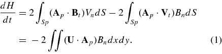
Here Ap is the vector potential of the magnetic fields; ▽ × Ap = B, which is uniquely specified by the observations on the surface; U denotes velocity measured in the photosphere,
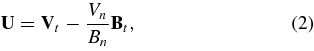
which includes both contributions from "true" horizontal mass motions on the solar surface (the first term) and a geometric effect of emergence of the magnetic field from the subsurface (the second term). It is worthy to note that the amount of helicity flux,
which is calculated by a proxy of helicity density, GA = −2(U · Ap)Bn, is very close to that using a better, more observationally useful, parameter,
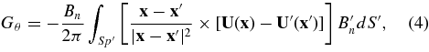
See Pariat et al. (2005, 2006) for more detail. One can find for AR 0656 that the results shown in Figure 4 are comparable with those from Jeong & Chae (2007) when using the Pariat et al. parameter Gθ.
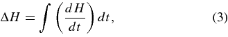
In using the LCT technique of Chae & Jeong (2005), we chose a typical window of 10'' and 96 minutes for the full width at half-maximum (FWHM) of the window function defining the extent of the local area and time difference Δt. The results from the LCT are combined with the field measurements to calculate the helicity injection rate dH/dt, and the total helicity flux ΔH injected into the corona over a period of 5 days, when the ARs are close to disk center, i.e., within ±40° heliographic longitude. We employ the same method as our previous paper (Tian & Alexander 2008), where a more detailed description can be found. However, in this paper, we separately calculate the contribution of positive and negative polarities to the helicity flux injected into the corona.
3. MAGNETIC STRUCTURE AND HELICITY INJECTION
We first investigate, in detail, the helicity flux injected by two ARs 8214 and 0656, which have corresponding recurrences 8227 and 0667+0670, respectively. These recurrent ARs are located within ±10° of the longitude of their parent ARs. The related information is shown in Table 1. The recurrent ARs can be confirmed by magnetograms found at the Big Bear Solar Observatory (BBSO) Active Region Monitor Web site1 by using the "rotation" survey.
3.1. NOAA 8214 and its Recurrent AR 8227
NOAA 8214 is observed as a newly emerging AR as it appears at the eastern limb. Its area increases rapidly from 40 area units (area units = 10−6 hemispheres of the solar disk) at N26E47 on April 30 to the largest area of 650 area units at N26W23 on May 5.2 It develops to be a well defined bipolar AR with an evident center of positive (negative) magnetic field as its leading (following) polarity. It rotated around the western limb on May 10, and then reappeared on the eastern limb on May 24, and was named as a new AR, NOAA 8227. We believe AR 8227 is a recurrence of NOAA 8214 based on the location of AR 8227 at N26L96 on June 1, which is very close to AR 8214 at N26L95 on May 4, (see also Bentley et al. 2000).
Figure 1 displays MDI 96 minute magnetograms of ARs 8214 (left) and 8227 (right). It is evident for AR 8214 that the magnetic field emerges very quickly and that the two opposite polarities separate rapidly. The leading polarity with positive flux (white patches) is more compact, while the following polarity with negative flux (black patches) is more dispersed and fragmented. Its recurrent AR, NOAA 8227, was observed as a decaying region. However, we can again note that the leading polarity with positive flux decayed more slowly and still contained a significant distribution of compact flux, while the following polarity with negative flux decayed and fragmented very quickly and dispersed over a large area.
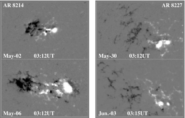
Figure 1. MDI/96 minute line-of-sight magnetograms of AR 8214 (N26L95, left) and AR8227 (N26L96, right). White (black) patches denote positive (negative) magnetic field. Size of images is 340 × 225 arcsec.
Download figure:
Standard image High-resolution imageThe development of the magnetic flux of the AR 8214 is shown in Figure 2(a), where the increase of the positive and negative fluxes is seen to be roughly similar. The correlation coefficient of the positive and negative fluxes is very high, Cr = 0.997, for 75 data points (see Figure 2(b)). A slope of the best linear fit, k, is 1.69, indicating that the increase of the positive flux is significantly faster than that of the negative flux.
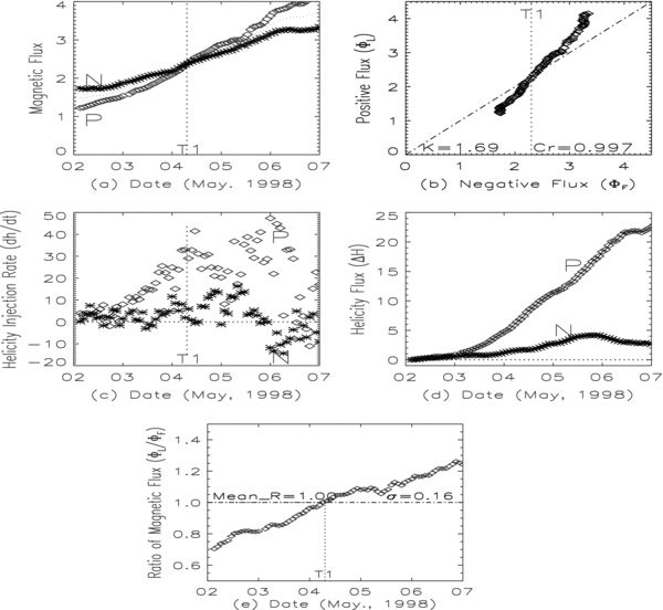
Figure 2. (a) Total radial magnetic flux (1022Mx) of positive ("◊") and negative ("*") polarities; (b) leading (positive) flux vs. following (negative) flux. (c) helicity injection rate (1040Mx2/h) of the positive ("◊") and the negative ("*") polarities; (d) their total helicity flux (1042Mx2) over 5 days; (e) development of the ratio of the leading and following flux. The vertical dotted lines at "T1" denote the time when the positive and negative flux is balanced. The other dotted lines denote development of mean flux in part (a) (i.e., (|ΦL| + |ΦF|)/2), magnetic flux balance in part (b), and a mean value of ratio of |ΦL|/|ΦF| in part (e). ``σ" denotes a standard deviation.
Download figure:
Standard image High-resolution imageThis emerging AR is a good example with which to study helicity injection and related topics because we can follow its development from almost the beginning of its emergence to several days later including the passage across the central meridian (i.e., over a longitudinal change from 40E to 40W). We employ the same method and LCT technique as used in Tian & Alexander (2008) to calculate the radial magnetic flux, helicity injection rate, and total helicity flux over 5 days spanning central meridian passage. Here, we distinguish the contribution from positive and negative polarities to the overall coronal helicity. Because the AR possesses a well defined bipolar magnetic structure, the contribution of positive (negative) flux to the coronal helicity can be considered to be that of the leading (following) polarity. The helicity injection rate and helicity flux injected by the leading (positive) and following (negative) polarities are separately shown in Figures 2(c) and 2(d), where "◊" (P) and "*" (N) denote values related to positive and negative fluxes, respectively. From the figure, we find that the positive leading polarity contributes at least seven times more helicity flux than that of the negative following polarity.
We can find from Figure 2(e) that the magnetic flux of the leading positive polarity and the following negative polarity is not balanced for the bulk of AR evolution over most of the time of observation. However, there is a transient balance at time "T1," i.e., magnetic flux of the leading polarity is equal to the magnetic flux of the following polarity. Comparing with Figure 2(c), the helicity injection rate of the positive leading polarity is much larger than that of the negative following polarity at all times. This indicates that the significant imbalance in the helicity injection rate and total helicity flux (see Figures 2(c) and 2(d)) is not directly related to the imbalance of the magnetic flux, though we show later that the magnetic flux imbalance is likely to result in the helicity flux imbalance.
We also see in Figure 2(c) that the measured helicity injection rate shows significant fluctuations in time, with the following polarity markedly varying in sign throughout the AR evolution. This is consistent with the recent simulation results of Y. Fan (2009, in preparation) where the fragmentation of the following leg of an emerging flux rope produces an untangling array of individual field lines with a mix of both positive and negative values of twist helicity. The distribution of helicities varies with length along the flux rope legs. A narrower distribution of helicity values, and all predominantly of the same sign, is seen for the leading polarity. If we assume that the structure simulated by Fan emerges to produce a bipolar AR, we would expect to see a picture similar to that shown in Figure 2(c), namely, an imbalance, coupled to strong fluctuations, in the helicity injection rate with the sign of the following polarity varying with time.
Considering that the tilt of the axis of the whole AR to the equator and its clockwise rotation are very small, the writhe helicity (related to the tilt angle), and the writhe helicity flux (related to the change of the tilt angle) injected into the corona should also be small, since the total helicity is a sum of twist helicity and writhe helicity. Combining conclusions from Jeong & Chae (2007) and Tian & Alexander (2008), that the coronal helicity originates predominantly from the emergence of magnetic field in the solar interior, and the result from this paper, that the leading polarity injects much more helicity flux into the corona, we argue that significantly larger twist helicity in the leading leg of the emerging flux tube can maintain the cohesion of the leading polarity field against possible sources of distortion (e.g., turbulence in the upper levels of the convection zone).
3.2. NOAA 0656 and its Recurrent ARs 0667 and 0670
NOAA 0656 (S13L83) is also a fast-emerging bipolar AR when it appears around the eastern disk. Its area increases quickly from an initial 250 area units at S13E58 on August 7 to its largest value of 1360 area units at S13W22 on August 13. It rotated around the western limb on August 18, and then reappeared on September 1, and was named NOAA 0667 (S13L93) with 0670 (S13L83), having split into two separate regions. The recurrent ARs are located using the X- and Y-coordinates associated with AR 0656 but one rotation later. MDI 96 minute magnetograms of ARs 0656 (left) and 0667 + 0670 (right) are shown in Figure 3. From the figure it is evident for AR 0656 that the leading polarity with negative flux is more compact, emerges strongly, and moves fast, while the following polarity, with positive flux, is dispersed and fragmented. Its recurrent AR, NOAA 0667+0670, is decaying, with the leading polarity decaying more slowly and remaining more compact than the following polarity. This AR maintains its leading polarity (see Figure 3) better than that of NOAA 8214 to NOAA 8227 (see Figure 1), while the fragmentation of the following polarity is similar, i.e., very dispersed.
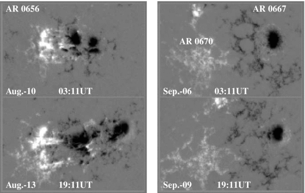
Figure 3. MDI/96 m line-of-sight magnetograms of ARs 0656 (S13L83, left) and 0667+0670 (S11L93–L83, right). Size of images is 320 × 210 arcsec.
Download figure:
Standard image High-resolution imageFigure 4 displays the evolution of the positive and negative radial fluxes (Figure 4(a)), the ratio of magnetic flux increase of the leading and following polarities (Figure 4(b)), helicity injection rate (Figure 4(c)), and helicity injection flux (Figure 4(d)) over a period of 5 days spanning central meridian passage. The result of the helicity flux (Figure 4(d)) indicates that the leading (negative) polarity injects a large amount of negative helicity flux into the corona, while the following (positive) polarity injects a much smaller amount of positive helicity. Once again we see significant fluctuations in the helicity injection rate (see Figure 4(c)) with the rate for the following positive polarity varying in sign over the observation period. For this AR, these fluctuations result in a cumulative helicity injection in the fragmented following polarity that is of opposite sign to that of the compact leading polarity (see discussion). It is evident that the magnetic flux increase of the leading polarity is much larger than that of following polarity (see Figure 4(b)), a ratio of 2.90. Moreover, the magnetic flux of the leading polarity is larger than that of the following polarity after the time "T1," i.e., for most of time during the 5 days of observation (see Figure 4(e)). However, the leading negative polarity still has a higher helicity injection rate (see Figure 4(c)), even before the time "T1," when the magnetic flux of the leading polarity is lower than that of the following polarity. This again reflects the weak relationship between the imbalance of helicity injection flux and magnetic flux imbalance. During the 5 days spanning the central disk, the imbalance of the leading and following magnetic flux has an average value 1.23 ± 0.19, as shown in Figure 2(e). Even taking into account the magnetic flux difference, we still find that helicity flux injected by the leading polarity is at least 12 times (H ∼ Φ2) larger than that of the following polarity. This implies significantly faster emerging motions of the leading polarity (see Equations (1) and (2)). Similar to the results for AR 8214 we suggest that the 7–20 times larger twist helicity in the leading leg of the flux tube is related to much better flux coherence in the leading magnetic field.
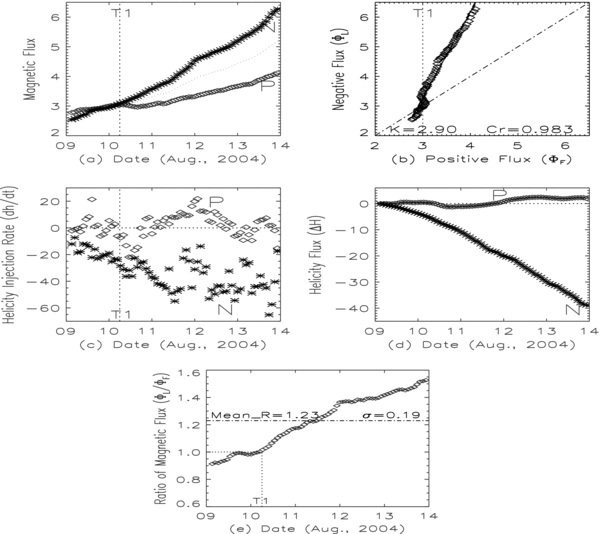
Figure 4. Same as Figure 2, but for AR 0656.
Download figure:
Standard image High-resolution image3.3. Helicity Injection Rate and Helicity Flux of Eight Emerging ARs
We use the same analysis described in Sections 3.1 and 3.2 to calculate the total magnetic flux, helicity injection rate and helicity flux of eight emerging ARs. Figure 5 displays the results of four ARs located in the southern hemisphere, that the injection rate and helicity flux over 5 days of the negative (leading) polarity tend to be much larger than that of the positive (following) polarity. Figure 6 displays the results of four ARs in the northern hemisphere, that the helicity injection rate and the helicity flux of the positive (leading) polarity tend to be much larger than the negative (following) polarity. The corresponding MDI 96 minute line-of-sight magnetograms of the eight ARs are shown in Figure 7, when the ARs were crossing the central meridian. From the Figure, we find that the following polarity in these strongly emerging bipolar ARs tends to be more dispersed and fragmented than the more compact leading polarity. Comparing results obtained in Figures 5 and 6, we find that the more compact leading polarity tends to have a much higher helicity injection rate and total helicity flux over 5 days than the more dispersed and fragmented following polarity. The result is same to that found in ARs 8214 and 0656 (see Figures 2(c) and 4(c)).
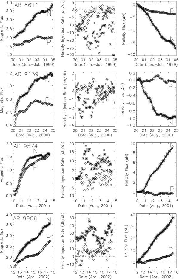
Figure 5. Development of magnetic flux, helicity injection rate, and helicity flux of ARs 8611, 9139, 9574, and 9906 located in the Southern hemisphere. "*" denotes negative flux (leading polarity), while "◊" denotes positive flux (following polarity). Others are same as Figure 2.
Download figure:
Standard image High-resolution image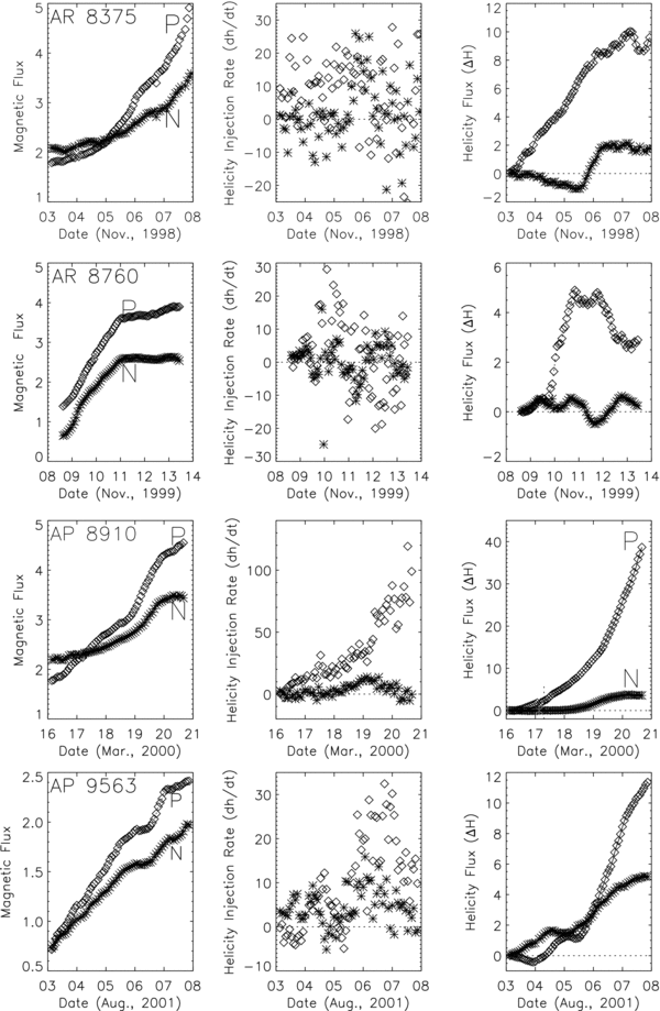
Figure 6. Development of magnetic flux, helicity injection rate, and helicity flux of ARs 8375, 8760, 8910, and 9563 located in the Northern hemisphere. "*" denotes negative flux (following polarity), while "◊" denotes positive flux (leading polarity). Others are same as Figure 2.
Download figure:
Standard image High-resolution image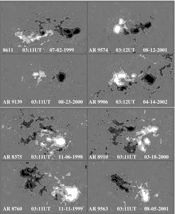
Figure 7. MDI/96 minute line-of-sight magnetograms of NOAA 8611 (S25), 9139 (S10), 9574 (S04), and 9906 (S15) in the Southern hemisphere, and 8375 (N19), 8760(N14), 8910 (S12) and 9563 (N23) in the Northern hemisphere. The contours are 200 G and 1000 G. The size of images is 300 × 180 arcsec.
Download figure:
Standard image High-resolution imageThe study of the above 10 emerging ARs signifies that in the bipolar strongly emerging ARs considered the leading polarity injects much more helicity flux into the corona than the following polarity. This is associated with the general magnetic configuration for such ARs that the leading magnetic field remains more compact and maintains a coherent structure for longer, while the following polarity is easily dispersed and fragmented. We summarize the statistical results of the sample of 15 ARs in Table 2, all of which show strong emergence, with both the positive and negative magnetic fluxes developing almost synchronously, and significant helicity flux injection over 5 days. A more detailed description for the full sample can be found in Section 2.
In Table 2, ΦL/ΦF and ΔΦL/ΔΦF denote ratios of the magnetic flux and the magnetic flux increase of the leading and following polarities. It is found in most of the ARs that the mean magnetic flux of the leading polarity is, in general, larger than that of the following polarity (i.e., ΦL/ΦF > 1.0). However, for part of their evolution some ARs show a leading flux that is smaller than the following polarity (i.e., ΦL/ΦF < 1.0, reflected in the standard deviation "σ" in Table 2). The ratio may reflect real magnetic flux imbalance between the leading and following polarities, though there is some uncertainty in the flux measurements, for regions with very weak field (|B| < 20 G) and very strong field (|B|>3500 G). In the former, the sensitivity of MDI means that significant flux, if distributed across a large number of small flux elements, may not be accounted for, while for the latter, saturation in the MDI leads to an underestimate of the leading polarity flux. Moreover, for most of the ARs the increase of the leading flux is faster than that of the following flux (i.e., ΔΦL/ΔΦF > 1.0, see also Figures 2(b) and 4(b)), typically over 1.5 times. This ratio may suggest that the leading polarity generally emerges faster than the following polarity. Consequently, the fast emergence results in fast horizontal motions, which have been measured by the LCT technique and taken into account in the calculation of helicity flux (see Equations (1) and (2)). The limitations of the LCT technique will be discussed in detail in last discussion section below. In the seventh column of Table 2, ΔHL (ΔHF) denotes the helicity flux injected by the leading (following) polarities, respectively. It is found that ΔHL for eight of the ARs is over five times larger than ΔHF, while about two to four times larger for the other six ARs. Only one AR, NOAA 0050, has lower ΔHL than ΔHF. In order to "remove" the gross effects of the flux imbalance, we produce a flux-weighted helicity flux, ![$T_L/T_F=[\frac {\Delta H_{L}} {\Phi_{L}^2}]/[\frac {\Delta H_{F}}{\Phi_{F}^2}]$](https://content.cld.iop.org/journals/0004-637X/695/2/1012/revision1/apj294117ieqn2.gif) , which is shown in the last column of Table 2. This value denotes the ratio of turn numbers of the twist in the leading and following magnetic field, and shows a smaller but still large helicity asymmetry. This result strongly signifies a predominant contribution of the leading polarity to the coronal helicity, which we believe is responsible for the leading polarity remaining compact and dispersing slowly.
, which is shown in the last column of Table 2. This value denotes the ratio of turn numbers of the twist in the leading and following magnetic field, and shows a smaller but still large helicity asymmetry. This result strongly signifies a predominant contribution of the leading polarity to the coronal helicity, which we believe is responsible for the leading polarity remaining compact and dispersing slowly.
4. CONCLUSION AND DISCUSSION
Observations have shown that the leading magnetic field of bipolar ARs is more compact while the following polarity is more dispersed (see Bray & Loughhead 1979; Zwaan 1981; Fan et al. 1993; Canfield 1999; Fan 2004; Canfield & Russell 2007). Characterizing the asymmetry between the two polarities is the primary purpose of this paper. Our motivation is based on several studies on the origin of helicity (e.g., Jeong & Chae 2007; Tian & Alexander 2008), which suggest that significant emergence of the magnetic flux is a primary source of helicity in the corona. On the other hand, some models (Longcope et al. 1996; Abbett et al. 2000; Fan 2001) predict that only flux tubes with a certain amount of twist can survive the interaction with the surrounding plasma in the convection zone and maintain its integrity. Flux tubes with lower twist do still emerge, but with a significant loss of flux (Fan 2008), and so a detailed analysis of AR asymmetry is essential to compare with the predictions of the models. We presume, based on these results, that the integrity of an emerging flux tube would be maintained more readily if the flux tube possessed more twist. At the other extreme, the kink instability would occur if the twist in the flux tube exceeds a critical value (see Fan et al. 1999; Linton et al. 1999; Tian et al. 2005).
If there is a different amount of the twist in the leading and following legs of a flux tube, the related magnetic field should have different morphology between the two polarities due to differences in the associated tension force. Since the leading (following) polarity is observed to be more compact (dispersed), it is reasonable to assume that more (less) twist exists in the leading (following) legs of a presumed Ω-shaped flux tube. Thus, the leading and following polarities would transfer more (less) helicity flux into the corona via the flux emergence, which can be measured by the LCT technique adopted here. Based on this consideration, in this paper, we separately calculate the helicity flux injected by the leading and following polarities for 15 emerging ARs using MDI 96 minute line-of-sight magnetograms and an LCT technique code developed by Chae & Jeong (2005), and find that the leading polarity does indeed inject several times more helicity flux than the following polarity. This result implies that the leading magnetic field of the Ω-shaped flux tube could possess a larger amount of the twist than the following one prior to the emergence. The more twist in the leading magnetic field would effectively protect the flux from disruption by turbulent convection motions, thus maintaining the magnetic tube coherence and limiting its dispersal.
Most of the ARs used in this paper provide excellent examples for studying topics of helicity injection, because they are relatively simple bipolar structures and we can follow their development from roughly the beginning of the emergence to several days later as they cross the meridian. The rotation of the whole AR, i.e., one polarity rotating around another one, is not evident in most of the ARs considered. Thus, the writhe helicity flux injected over the 5 days is expected to be small. On the other hand, the helicity flux contributed by the horizontal motions of the photospheric mass and differential rotation is not significant (see Tian & Alexander 2008; and references therein). Consequently, we can assume that the helicity flux calculated by the LCT technique primarily includes the twist helicity flux that emerges from subsurface.
It is worth noting that there are some limitations in using the LCT technique, such as lower resolution of the MDI magnetograms, magnetic field saturation in umbrae, and underestimation of twisting motions such as sunspot rotation (see Démoulin & Berger 2003 and Gibson et al. 2004 for more detail), which may affect the calculation of the helicity injection rate and total helicity flux. The lower resolution of MDI magnetograms would underestimate the contribution from the weak field, especially in the dispersed and fragmented following polarity, while the magnetic field saturation in umbra would underestimate the contribution from the stronger feld than 3500 G, especially in the more compact leading polarity. Moreover, the LCT technique faces significant difficulties in regions such as sunspot umbra where the field distribution has small spatial variation and hence the data do not provide enough information to follow individual flux tubes. Additionally, sunspot rotation could be an important source of coronal helicity, which would be seriously underestimated, because the LCT technique is not effective at measuring the twisting motions of photospheric mass. This underestimation should be more evident in the leading polarity because the compact leading polarity tends to rotate more strongly than the following polarity based on implication of some observations (see Brown et al. 2003; Longcope & Ravindra 2007; Tian et al. 2008; Yan et al. 2008). It should also be noted that using a proxy, GA, for the helicity flux density in the LCT technique could give a spurious signal, which usually occurs in big sunspots (more compact polarity, see Pariat et al. 2006 and Nindos et al. 2003). However, Pariat et al. (2006) claimed that the helicity injection rate differs little between measurements using the GA or the more observationally attractive parameter Gθ (see Equation (6) and Table 1 of Pariat et al. 2006 for more detail). Though we cannot quantify exactly how much the limitations of the LCT approach and the constraints of the MDI data contribute to the underestimation of the helicity injection rate and total helicity flux, we believe that the extremely large difference of the helicity injection rate and total helicity flux measured between the leading and following polarities is physical in origin and signifies a real consequence of the dynamics in the solar interior. Our overall result, that there is a marked difference in the magnitude and distribution of the helicity flux between the two polarities provides physical basis for the observed morphological difference in these bipolar ARs. This assertion is further supported both by the result discussed in Section 4.3, that the rate of emergence and the proper motion of the leading polarity is larger than that of the following polarity, which is a same conclusion to that obtained previously (see Chou & Wang 1987; van Driel-Gesztelyi & Petrovay 1990; Petrovay et al. 1990), and by models of flux emergence in which magnetic tubes with a higher degree of twist (and therefore greater magnetic tension) have higher rates of emergence into the atmosphere (see Murray & Hood 2008; Cheung et al. 2008). This result will also hopefully be confirmed by new observations from Hinode and SDO with high spatial resolution and vector magnetograms.
It is interesting to note that in six of the 15 ARs, NOAA 0488, 8611, 8771, 9574, 0365, and 0656, the leading and following polarities inject opposite integrated helicity fluxes over the 5 day period of our measurements. We argue this could be due to the increased fragmentation on the magnetic field on the following side. The fragmentation results in smaller magnetic flux elements that are then more vulnerable to the turbulent dynamics of the upper levels of the convection zone. This results in the increased dispersion of the flux elements and could also possibly result in a redistribution of the twist such that the following polarity is comprised of a mix of flux elements with a range of intrinsic twist values, including twist of opposite sign. This latter conjecture is borne out in part by the simulations of Y. Fan (2009, in preparation), which show that the following leg of the emerging flux rope unravels along its length with individual field lines having a wide range of twist and helicity values, of both signs, at any given depth. The assumption is that as this flux rope emerges the helicity flux of the following polarity would be reflected in the dominant sign associated with that particular part of the flux rope. The net effect is that the cumulative helicity flux would be measured to be significantly lower in the following polarity than in the leading polarity and would fluctuate in sign as the emergence proceeded, as observed in the present work. The mixed sign of the twist raises some interesting questions regarding the current systems in the AR and the implications that such systems might have for magnetic reconnection and associated flare and coronal mass ejection (CME) productivity of the AR. This is beyond the scope of the present analysis but will be considered in future work. While this result has interesting correspondences with what is expected from the simulations, it is possible that the opposite sign could result from employing the helicity flux density GA to calculate the helicity injection rate and total helicity flux: a more detailed explanation can be found in Pariat et al. (2006; see also Figure 5). To address this possibility observationally will require the higher resolution and vector magnetic field capability of Hinode and SDO. We plan a future statistical study based on accumulated observations from these two spacecraft as the statistical samples increase.
4.1. Vertical Current Imbalance in Solar Active Regions
The source of the energy released in solar flares is believed to be free magnetic energy stored in ARs. In particular, the energy is thought to derive from the nonpotential component (e.g., twist) of the magnetic field, which generates a current system that flows along the axis from one footpoint of a flux tube crossing the corona back to the other footpoint. It has been found that the emergence of electrical currents with magnetic flux, rather than surface shear flows or other purely atmospheric effects, appears to be key in driving AR flaring (e.g., Melrose 1995; Wheatland 2000; Schrijver et al. 2005).
Wheatland (2000) used vector magnetograms in the photosphere and found that nonneutralized current exists in most (13/21) of the ARs he studied, i.e., one polarity of an AR possesses a positive vertical current while the opposite polarity possesses a negative vertical current. The current can cause a line-of-sight flux imbalance because of the directionality of the magnetic field they produce (see Gary & Rabin 1995). Moreover, Moore (2008) has also shown recently that the currents in the two polarities may not be balanced with the current being stronger in the leading polarity. We use Huairou vector magnetograms to calculate the vertical current for AR 8214, and find that the total vertical current is also imbalanced in this AR: 0.23 ± 0.02 × 10¹²A for the leading polarity and −0.16 ± 0.01 × 10¹²A for the following polarity. This result implies that the current helicity (∫∫BzJzdxdy) could also not be balanced since the magnetic flux of the leading polarity tends to be larger than that of the following polarity. Thus, both the current and twist helicity in the leading polarity tends to be stronger than in the following one. However, modern vector magnetograms are not good enough to be used quantitatively, due to considerable uncertainties such as reliability of the transverse field, resolution of the 180° ambiguity, effect of Faraday rotation, and large noise in transverse field. We can expect to get good vector data from SDO/HMI, together with Hinode, to investigate the imbalance of the vertical current, current helicity, helicity flux, and/or other twist parameters, for an AR at the same time in the future. The significant imbalance of the helicity flux observed in this paper may provide evidence supporting the current imbalance, since both reflect the same physical character.
4.2. What is the Physical Origin of the Helicity Flux Asymmetry?
The main result of this paper is that the leading polarity injects a much larger component of the total helicity flux than the following one. Although the study could be affected by the limitations of the use of MDI line-of-sight magnetograms in both very weak (|B| < 20 G) and very strong (|B|>3500 G) field regions due to the observational noise and flux saturation, respectively, and the immaturity of the LCT techniques, the large observed difference of the helicity flux, over a factor of 10 in some ARs (8760, 8910, 9139, 9574, and 0656; see Table 2), between the leading and following polarities, should be physical in origin (see above). Magnetic flux imbalance will contribute somewhat to this, but should not be the major source, because we find, in some ARs, that even when the leading flux is smaller than the following flux, the helicity injection rate is still much higher in the leading polarity (see Figures 2(c) and 2(e), 4(c) and 4(e), the last column in Table 2, and the analysis in Section 3).
This result implies that the leading leg of a presumed Ω-shaped flux tube possesses more twist than that of the following leg prior to its emergence from the interior. If the twist of the magnetic field is produced by dynamo action in the solar interior, what processes generate the twist asymmetry? Longcope & Welsch (2000) predicted a particular behavior of twist depending on the rate of the flux tube emergence, i.e., the level of rotation of the footpoint of the flux tube will depend upon the rapidity of flux emergence. This would imply, from the ratio of ΔΦL and ΔΦF shown in Table 2, that the leading polarity emerges faster than the following one, over 1.5 times as fast. Though present observations do not supply enough data to investigate if the leading sunspot rotates more strongly than the following sunspot, a number of observations (Brown et al., 2003; Longcope & Ravindra, 2007; Tian et al. 2008; Yan et al. 2008) clearly show this implication. Based on the work of Longcope & Welsch (2000), the results shown in Table 2 imply that the leading polarity should rotate faster and thereby produce more helicity. Therefore, the leading polarity possesses more helicity so that the leading flux is maintained to be compact and cohesive, due to a stronger tension of the magnetic field, and consequently, is less affected by the convective motions. The opposite situation occurs in the following polarity: slow flux emergence related to slow rotation and so less helicity, due to which the following field is seriously affected by the convective motions, resulting in dispersal and fragmentation with the helicity injection flux characterized by having large fluctuations. Y. Fan's (2009, in preparation) simulation does find that there is a systematically greater magnitude of helicity injection rate compared to the following at all depths when a flux tube rises in the solar interior.
4.3. Does the Leading Polarity Move and Emerge Faster?
The magnetic flux of the leading polarity increases faster than that of the following flux, which is characterized by the ratio ΔΦL/ΔΦF shown in Table 2. Faster emergence in the leading polarity can result in more rapid horizontal motions in the photosphere. Such asymmetric proper motions have previously been observed in young ARs and sunspot groups (see Chou & Wang, 1987; van Driel-Gesztelyi & Petrovay, 1990; Petrovay et al., 1990), supporting the observations reported in this paper. Fan et al. (1993) explained that as the field strength in the leading leg becomes proportionately stronger, it becomes more buoyant. Moreno-Insertis et al. (1994) and Caligari et al. (1995) argued that the asymmetric proper motions are due to geometrical asymmetry of the Ω-shaped flux tube, with the leading leg being inclined more horizontally than the following leg. This field strength asymmetry may explain the observed more compact morphology of the leading polarity compared to its following polarity.
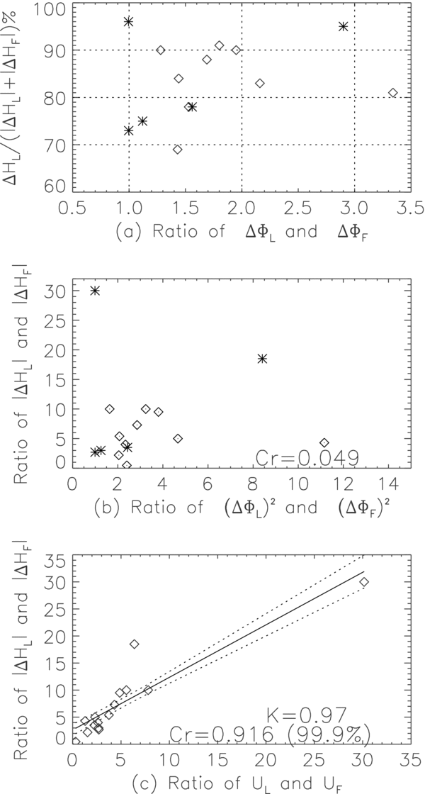
The overall movement of the magnetic field elements can be roughly estimated based on Equation (1), which indicates ΔH ∝ U · ΔΦ2, where ΔH, U, and ΔΦ denote helicity flux injected, overall speed, and the increase of the magnetic flux, respectively. Thus, ratios related to the leading and following polarities are of the form
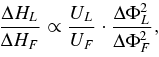
and
where subscripts "L" and "F" denote associated parameters of leading and following polarities. Figure 8(a) shows that the helicity flux imbalance ( ) of 14 ARs is over 65%, except NOAA 0050; the imbalance in nine ARs is over 80%. Figure 8(b) shows that the asymmetry of helicity flux (
 ) injected by the leading and following polarities has little relationship with the square of the ratio of the magnetic flux increase; a small correlation coefficient of 0.049. However, the asymmetry of helicity flux is highly correlated to the speed asymmetry (
 ); a much larger correlation coefficient of 0.916 with a confidence level >99.9%. These rough relationships suggest that the leading polarity with more helicity emerges and also moves horizontally faster than the following polarity, which is same to that obtained previously (see Chou & Wang 1987; van Driel-Gesztelyi & Petrovay 1990; Petrovay et al. 1990), and supports the prediction of Longcope & Welsch (2000) discussed above. Consequently, the leading leg of the presumed Ω-shaped flux tube rotates faster than the following leg, producing more helicity that can maintain its magnetic field lines more cohesively due to the stronger magnetic tension force. The result reported here supports the ideas that the asymmetry of helicity flux indeed exists between the leading and following magnetic field, and is related to the difference of the emerging speed of the two legs of the inclined Ω-shaped flux tube. Moreover, Murray & Hood (2008) found that magnetic tubes with higher degree of twist (and therefore greater magnetic tension) have higher rates of emergence into the atmosphere, which is also supported by a model result of Cheung et al. (2008). Our observational conclusions are consistent with that of these models.
Figure 8. Relationship among magnetic flux, helicity flux, and overall velocity of leading and following polarities. "*" ("◊") denotes active regions of which the leading helicity flux follows the hemispheric helicity rule, negative (positive) in the Northern (Southern) hemisphere.
Download figure:
Standard image High-resolution image
The authors would like to thank P. Démoulin, R. Moore, and Y. Fan for valuable discussions and suggestions, and are grateful to the Huairou and SOHO teams for producing such wonderful data. This research is supported by NASA grant NNX07AH38G.