


ABSTRACT
We examine the interaction of three coronal mass ejections (CMEs) that took place on 2012 March 5 at heights less than 20 R⊙ in the corona. We used a forward fitting model to reconstruct the three-dimensional trajectories and kinematics of the CMEs and determine their interaction in the observations from three viewpoints: Solar and Heliospheric Observatory (SOHO), STEREO-A, and STEREO-B. The first CME (CME-1), a slow-rising eruption near disk center, is already in progress at 02:45 UT when the second CME (CME-2) erupts from AR 11429 on the east limb. These two CMEs are present in the corona not interacting when a third CME (CME-3) erupts from AR 11429 at 03:34 UT. CME-3 has a constant velocity of 1456[±31] km s−1 and drives a shock that is observed as a halo from all viewpoints. We find that the shock driven by CME-3 passed through CME-1 with no observable change in the geometry, trajectory, or velocity of CME-1. However, the elevated temperatures detected in situ when CME-1 reached Earth indicate that the plasma inside CME-1 may have been heated by the passage of the shock. CME-2 is accelerated by CME-3 to more than twice its initial velocity and remains a separate structure ahead of the CME-3 front. CME-2 is deflected 24° northward by CME-3 for a total deflection of 40° from its source region. These results suggest that the collision of CME-2 and CME-3 is superelastic. This work demonstrates the capability and utility of fitting forward models to complex and interacting CMEs observed in the corona from multiple viewpoints.
Export citation and abstract BibTeX RIS
1. INTRODUCTION
Coronal mass ejections (CMEs) are the largest and most dynamic propagating structures in the corona and heliosphere. It has long been known that CMEs can interact with each other as they propagate through interplanetary space. In the early days of space physics, such interactions were suggested by in situ data of the interplanetary medium (Intriligator 1976; Ivanov 1982; Burlaga et al. 1987). The interaction of two or more CMEs or their driven shocks (CME–CME interaction) is a logical assumption given the rate, more than four per day, of CMEs produced from the Sun during times of high solar activity (Yashiro et al. 2004) and that many active regions will produce multiple CMEs within hours of each other. The first published observations of a CME–CME interaction in the white-light coronagraph data were made using the Large Angle and Spectrometric Coronagraph (LASCO; Brueckner et al. 1995) instruments on board Solar and Heliospheric Observatory (SOHO; Domingo et al. 1995). Gopalswamy et al. (2001) inferred the interaction of two CMEs by combining the LASCO observations with long-wavelength radio emission observations. Due to projection effects, it is often very difficult to confirm CME–CME interactions in single-viewpoint white-light observations without significant deflections or the addition of other data sources such as radio or in situ observations (Burlaga et al. 2002, 2003; Wang et al. 2002).
Our ability to study CME–CME interactions has increased significantly with the launch of the twin Solar Terrestrial Relations Observatory (STEREO; Kaiser et al. 2008) spacecraft in 2006 October. Using the multiple-viewpoint white-light observations from the Sun–Earth Connection Coronal and Heliospheric Investigation (SECCHI; Howard et al. 2008) instrument suites, several CME–CME interactions have been observed and studied. Recent studies of CME–CME interactions include events from 2008 November 2–8 (Shen et al. 2012), 2010 May 23–24 (Lugaz et al. 2012), 2010 August 1 (Harrison et al. 2012; Liu et al. 2012; Temmer et al. 2012), 2011 February 13–15 (Maričić et al. 2014; Mishra & Srivastava 2014; Shanmugaraju et al. 2014; Temmer et al. 2014), 2012 November 9–10 (Mishra et al. 2015), and 2012 September 30–October 1 (Liu et al. 2014b). All of these CME–CME interactions were observed within the wide-angle field of view (FOV) of the Heliospheric Imagers (HIs) on STEREO at a height greater than 20 R⊙. Additionally, a majority of these studies used single-viewpoint J-maps (Sheeley et al. 1999) of the SECCHI data to track the propagation and interaction of the CMEs. Studies of CME–CME interactions in the corona are limited. Liu et al. (2014a) and Yashiro et al. (2014) reported on CME–CME interactions that took place near the Sun, observed in the SECCHI COR1 FOV.
CME–CME interactions are of interest because of their impact on many areas of heliospheric research. One of the most basic open questions regards the nature of these collisions; are they inelastic, elastic, or superelastic? Some studies indicate that the collisions may be superelastic (Shen et al. 2012), while others find that they may create radio emissions (Gopalswamy et al. 2002a; Shanmugaraju et al. 2014). Lugaz et al. (2012) report a perfectly inelastic collision, while Mishra & Srivastava (2014) find an inelastic, but nearly elastic, collision. CMEs can also affect each other without colliding, for example, by changing the local environment through which a subsequent CME propagates. These interactions may reduce drag and thus prevent deceleration for the following CME (Temmer & Nitta 2015), or they enhance particle acceleration (Gopalswamy et al. 2002b; Ding et al. 2014) or not (Kahler & Vourlidas 2014). This lack of understanding, combined with observations that show that CME–CME interactions can greatly alter the trajectory, morphology, kinematics, and magnetic structures of the individual events (Temmer et al. 2014; Mishra et al. 2015), creates multiple challenges to accurate space weather forecasting.
Another open question relevant to space weather forecasting is how the CME–CME interaction changes the geo-effectiveness of these events at Earth. The most extreme events of the last two solar cycles, the 2003 October–November and 2012 July events, were the result of multiple interacting CMEs released from the same active regions (Gopalswamy et al. 2005; Liu et al. 2014a). These events suggest that CME–CME interaction may play a role in large geomagnetic storms. Kamide et al. (1998), Farrugia et al. (2006), and Zhang et al. (2008) all suggest that combined CMEs might cause multistep major geomagnetic storms. However, without knowledge of the exact CME–CME interaction of individual events, it is unlikely that we will be able to accurately predict their geo-effectiveness.
Remote sensing observations of CME–CME interactions provide only kinematic or dynamical information. To determine how the magnetic field and plasma change as a result of the interaction, we must rely on magnetohydrodynamic (MHD) simulations. There have been many MHD simulations of CME–CME interactions (e.g., Lugaz et al. 2005; Wang et al. 2005; Xiong et al. 2007). However, few of these studies have attempted to compare with or reproduce observed events (Lugaz et al. 2007; Wu et al. 2007; Shen et al. 2013, 2014). To expand our understanding of CME–CME interactions through MHD studies of real events requires accurate and comprehensive measurements of observations. However, the very nature of these interactions makes such measurements difficult to obtain. The interaction may distort the CME structures and confuse their in situ signatures, thus complicating their detection at Earth. Near the Sun, interacting CMEs being ejected in close temporal proximity often overlap in coronagraph images, making it difficult to obtain accurate properties (e.g., speed, width, mass) for the individual events. These measurements are, however, essential for initializing CME propagation codes and simulations, and inaccurate or misidentified measurements of the observations impede accurate forecasting of their properties at Earth.
Many of the difficulties with measuring CME–CME interactions can be overcome by using multiple-viewpoint observations. However, past studies using STEREO observations have not taken full advantage of these data. Many of these studies have used the STEREO multiple-viewpoint observations to locate the initial three-dimensional (3D) trajectory and velocity of the individual CMEs (Temmer et al. 2014; Mishra et al. 2015). However, the CME–CME interaction takes place in the HI FOV, where 3D reconstruction is less accurate (Lugaz et al. 2010). Ding et al. (2014) demonstrated the application of using 3D reconstruction techniques in the FOV of the coronagraphs for a relatively simple CME–CME interaction on 2013 May 22. They concluded that this interaction produced a strong enhancement in the Type II radio burst and contributed to the particle acceleration from this event. However, no one, to our knowledge, has ever attempted to simultaneously reconstruct more than two CMEs.
In this paper, we demonstrate that 3D reconstructions of overlapping and interacting CMEs not only are possible but also provide crucial information about the interaction and evolution of the events and help us understand both the coronal evolution and the in situ signatures of the events at Earth. To this purpose, we selected three CMEs observed together on 2012 March 5 at heights below 20 R⊙. We analyzed multiple-viewpoint observations of these CMEs to reconstruct their 3D geometry and kinematics and determine their interaction. As these CMEs propagate into the corona, we are able to measure the changes in direction and velocity due to their interaction. We then examine the in situ observations associated with these events and their geo-effectiveness.
In Section 2, we describe the various observations and analysis methods used and the appearance of each CME before the interactions are observed. In Section 3, we discuss the interactions of the CMEs in the corona. We examine the in situ signature of these CMEs at Earth and the space weather impact of these events in Section 4. We conclude in Section 5 by comparing our results with past studies and summarize our results.
2. OBSERVATIONS AND METHODS
Our analysis relies primarily on coronagraph observations from the three available viewpoints: near Earth at the L1 point, SOHO, and the two STEREO spacecraft. On 2012 March 5, the STEREO spacecraft, STEREO-A (STA) and STEREO-B (STB), were 109° and −118° from Earth, respectively. Although the large angular separation from the Sun–Earth line is not ideal for observing Earth-directed CMEs in the heliosphere, it offers a suitable viewing perspective for the study of CMEs in the corona. As we will show, the interaction of the three CMEs takes place within the FOV of the coronagraphs. To derive the 3D properties of the events, we simultaneously analyze the observations from all six coronagraphs of the LASCO and SECCHI instrument suites. The SECCHI coronagraphs, COR1 and COR2, have overlapping FOVs at 1.5–4.0 R⊙ and 2.5–15 R⊙, respectively. LASCO C2 and C3 have similarly overlapping FOVs at 2.2–6.0 R⊙ and 3.8–32 R⊙, respectively.
With multiple viewpoints, we are able to fit the geometry of the CMEs with the graduated cylindrical shell (GCS) model (Thernisien et al. 2009) and track their 3D trajectories by making these fits over the duration of the observations. The projections of the CMEs look significantly different from each viewpoint, allowing us to fit the GCS model to the observations with a high degree of certainty. From the GCS model fit parameters, we infer the trajectories, orientations, velocities, and source regions (SRs) of the CMEs.
All three CMEs are from SRs on the Earth-facing hemisphere of the Sun; to confirm the SRs indicated by the GCS fits, we examined the extreme-ultraviolet (EUV) observations from both STEREO/SECCHI EUVI and the Atmospheric Imaging Assembly (AIA) on board the Solar Dynamics Observatory (SDO; Lemen et al. 2012). The quiet-Sun prominence eruption associated with CME-1 was observed in the 304 Å images from EUVI-A, EUVI-B, and AIA. The SR of CME-2 and CME-3, AR 11429, was well observed in all the coronal wavelengths of AIA. The high temporal and spatial resolution of AIA allows us to identify the separate eruptions in the SR that lead to the initiation of these two CMEs.
2.1. First CME (CME-1)
On 2012 March 4 at 23:05 UT, CME-1 emerges in the NE (NW) quadrant of the COR1-A (B) FOV. CME-1 is a classic example of a "streamer blowout" type event (Howard et al. 1985), with a slow-rising phase associated with a quiet-Sun prominence eruption originating from below the cusp of a helmet streamer. The faint flux-rope like structure, also typical of these types of CMEs, can be seen in the top panels of Figure 1 at 02:20 UT on 2012 March 05. The bottom panels of Figure 1 show the GCS model fits (magenta) overplotted on the observations. At this time, the 3D height of the CME is fitted at 3.4 R⊙ in the COR1-A(B) and COR2-A (not shown) observations. (All observations and fits are available as a movie in the online journal). The 3D trajectory of CME-1 is north of the Sun–Earth line at N19E3. Thus, the CME is completely obscured by the occulter in the LASCO C2 FOVs. The footpoints of the model and the central axis of the "croissant" make an angle of 132° with the solar equator as measured counterclockwise from a right-handed axis. This angle is often referred to as the tilt of the model (Thernisien 2011).
Figure 1. Contemporaneous observations of CME-1 from COR1-B (left), LASCO C2 (center), and COR1-A (right) and the GCS fit (magenta) overplotted for each viewpoint. CME-1 reached a height of 3.5 R⊙ before CME-2 is observed in the coronagraphs. We are able to continuously fit the observation of CME-1 with the GCS model, from its first emergence in COR1 until it leaves the COR2 FOV.
(An animation of this figure is available.)
Download figure:
Video Standard image High-resolution imageWe are able to fit all the observations of CME-1, from its first emergence in COR1 until it leaves the COR2 FOV. From these 3D height–time (HT) measurements, we derive the kinematic of CME-1 (see Section 3 for details). CME-1 initially rose with an average velocity of 100 km s−1. As expected for slow CMEs, it accelerates until it reaches a typical final speed of ∼550 km s−1 at 10 R⊙. Given the propagation of CME-1 at just 19° north of the Sun–Earth line, we expect CME-1 to impact Earth, and it is observed in situ. However, the CME–CME interactions create a complex in situ signature. We will examine the in situ observations associated with these CMEs in Section 4.
From the GCS fit, we determined that the SR of CME-1 is in the northern hemisphere near disk center as seen from Earth. We associate the eruption of CME-1 with a 304 Å prominence eruption observed throughout 2012 March 4 by SECCHI EUVI and SDO AIA. Figure 2(a) shows the pre-eruption prominence as observed by AIA on 2012 March 4 at 00:00 UT. The prominence has a clear NE–SW inclination, similar to the inclination of the footpoints of the GCS model fit. After the prominence erupts, it is observed above the limb from the STA and STB viewpoints in the EUVI 304 Å observations. This prominence was long-lived and very active; over the course of 2012 March 04, two other CMEs associated with the same SR were observed at 04:25 and 13:05 UT in the COR1 CME Catalog.3 Thus, this prominence is associated with at least three CMEs; CME-1 is the last CME associated with it. Figure 2(a) shows the prominence in an EUVI-B 304 Å image at 19:56 UT on 2012 March 4. For the next 2 hr, the prominence material is seen dissipating above the limb until it completely disappears from the EUVI-A (B) FOV at 22:46 UT. The timing of the prominence disappearance correlates well with the appearance of CME-1 in the COR1 FOV.
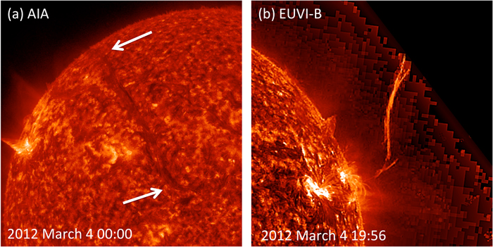
Figure 2. (a) AIA 304 Å image at 2012 March 4 00:00 UT of the pre-eruption prominence associated with CME-1 on disk. The NE–SW orientation of the prominence is similar to that of CME-1 footpoints derived from the GCS fit (Figure 1). (b) EUVI-B 304 Å image at 2012 March 4 19:56 UT of the CME-1 prominence eruption. The prominence completely disappears from the EUVI-A (B) FOV at 22:46 UT.
Download figure:
Standard image High-resolution image2.2. Second CME (CME-2)
At 02:45 UT on 2012 March 5, CME-2 appears in the COR1 observations. By this time, CME-1 has reached a height of 3.5 R⊙. CME-2 is much faster than CME-1 with a constant initial velocity of 576[±28] km s−1 and quickly reaches a similar height. CME-2 also has a moderate width of 46°. Figure 3 shows CME-1 and CME-2 observations from all six coronagraphs at heights of 4.4 and 4.1 R⊙ between 03:35 UT and 03:41 UT on 2012 March 05. The SR of CME-2 is NOAA AR 11429 located at N19E58 as observed from Earth. From the GCS model fit to the observations, the initial trajectory of CME-2 is N35E64. This is a considerably nonradial trajectory relative to the SR of 16° north in latitude and 6° east in longitude, but it is not unusual. CME-2 propagates toward the heliospheric current sheet, similar to other examples in Liewer et al. (2015). The GCS model footpoints are oriented at 68° from the solar equator; thus, the CME is primarily in the north–south direction. The tilt of the GCS model for CME-2 is most evident in the STA viewpoint (Figure 3, right).
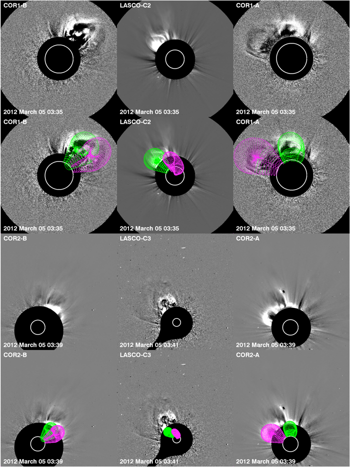
Figure 3. Contemporaneous observations of CME-1 and CME-2 in all six coronagraphs from STB (left), LASCO (center), and STA (right) before the eruption of CME-3. The GCS fits suggest that the CMEs do not interact. CME-1 (magenta) and CME-2 (green) are observed at 4.4 and 4.1 R⊙, respectively.
Download figure:
Standard image High-resolution imageFigure 3 shows the GCS fits of both CME-1 (magenta) and CME-2 (green). Based on the GCS fits to the observations, CME-1 and CME-2 are expanding into the corona without interacting. Given the size and location of the two CMEs, we would not expect them to interact. From the Earth and STB viewpoints, it is unclear that these CMEs are separated since they seem to overlap in these observations due to projection effects. However, from the STA observations it is clear that the CMEs are separated in the corona. We also note that the axes of CMEs are tilted opposite to each other (132° and 68°), consistent with the orientations of their respective SRs.
CME-2 has a very different appearance in the COR1-A and COR1-B views due to projection effects and the distortion of its front. The distortion of the front from smoothly curved is most apparent in the COR1-B and LASCO C2 observations. The northernmost part of the front seems to lag behind the southern front. The distortion makes it difficult to fit the GCS model over the full extent since the GCS model does not take into account distortions (to minimize the free parameters). After several tries, we chose to fit the height of the southern part of the front with the smooth edge of the GCS model because this fit best represents the data. The distortion of CME-2 is mostly likely due to the interaction with the nearby dense streamer that can be seen from the other viewpoints. Thus, the fit as seen from the COR1-A viewpoint does not match the data well. From the STA viewpoint, we are looking over the top of the CME and only see the lower northern front.
Figure 4 shows the SR of CME-2 (and CME-3), AR 11429 in the SDO AIA 171 Å observations. The observations reveal a set of loops rising at 02:10 UT. In Figure 4(a) we show the AR at 02:18 UT after the loops associated with CME-2 began to rise. In addition to the bright loops seen rising within the AR, there are also higher, fainter loops rising in the AIA 171 Å observations that we also associated with CME-2. This is only a partial eruption of the AR; the loops that will erupt later with CME-3 are present in SR before and after the eruption of CME-2. The CME-2 erupting loops appear to have a north–south orientation in the AIA observations roughly perpendicular to the orientation of the magnetic bi-pole of the AR. The orientation of these loops is similar to the orientation of the GCS model footpoints.
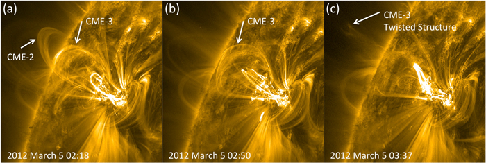
Figure 4. AIA 171 Å observations of AR 11429 (a) during and (b) after the eruption of the loops associated with CME-2. The CME-2 loops are oriented north–south, perpendicular to the magnetic axis of the AR and the CME-3 loops. The CME-3 loops persist in (a) and (b) until CME-3 erupts and a twisted structure (c) is seen rising from the AR. This eruption produced an X1.1 flare in the GOES-14 SXR data.
Download figure:
Standard image High-resolution imageThere was some flaring associated with the eruption of CME-2. However, the actual flare activity is difficult to determine owing to a high soft X-ray (SXR) background and the overlap with the X-class flare associated with CME-3 (see next section). The GOES-14 observations show the SXR level rising around 02:20 UT, reaching approximately M-class levels by 3:30 UT. The AIA 171 Å and 131 Å observations show flaring within the AR over a small part of the AR during this period. A detailed flare analysis is beyond the scope of this paper, so we tentatively associate this ∼M-class flare with CME-2.
2.3. Third CME (CME-3)
At 03:45 UT on 2012 March 5, CME-3 emerges into the COR1 FOVs. Its eruption from AR 11429 is accompanied by an X1.1 class X-ray flare. In the COR1-A (B) observations, CME-3 has a broad front and emerges quickly with a velocity of 1456[±31] km s−1. From the LASCO C2 viewpoint, the CME is seen edge-on and has a narrower width observed from the STEREO viewpoints. Figure 5 shows all three CMEs low in the corona at around 03:55 UT, along with the GCS models. These observations are before we see any clear signs of CME–CME interaction. At this time, CME-1, CME-2, and CME-3 are at heights of 4.7, 5.0, and 3.5 R⊙, respectively. CME-3 propagates nonradially from the SR with a trajectory of N27E58, similarly to CME-2. The tilt of CME-3 is at 157° from the solar equation and perpendicular to the orientation of CME-2. As CME-3 continues to emerge, the three CMEs begin to interact. We will analyze this interaction in the next section.
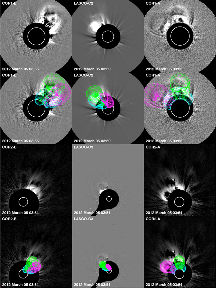
Figure 5. Contemporaneous observations showing CME-1, CME-2, and CME-3 at heights of 4.7, 5.0, and 3.5 R⊙ before the observed interactions. Streamer deflections in COR1-B (western limb) and LASCO C2 (eastern limb) indicate that CME-3 is driving a shock.
Download figure:
Standard image High-resolution imageIn the COR1-B image (Figure 5, top left), as CME-3 emerges, a streamer on the west limb appears as a black-and-white structure, indicating motion in these running difference images. A similar signature is seen on the east limb in the LASCO C2 image (Figure 5, top middle) for the same streamer. This is evidence of the shock produced by CME-3, although the white-light shock front is not yet visible in the observations. As CME-3 continues out into the corona, the driven shock becomes more prominent until it is visible in all the observations. CME-3 was classified as a halo from all three viewpoints in both the SOHO LASCO CME Catalog4 and the SECCHI COR2 CACTus Catalog.5 The shock affects the corona globally, and CME-3 begins to interact with CME-1 and CME-2 shortly after its emergence in the corona.
The eruption of CME-3 from AR 11429 is almost an hour after the eruption of CME-2 from the same AR. This eruption produced an X1.1 flare in the GOES-14 SXR data; the flare peaks at 04:00 UT, followed by a gradual decline over 2 hr. The loops that erupt with CME-3 were present in the AR for several hours, before, during, and after the eruption of CME-2, as shown in Figure 4. Figure 4(b) shows these loops between the eruption of CME-2 and CME-3 at 02:50 UT in a seemingly stable configuration. At 03:32 UT, a twisted structure is seen erupting in all the coronal wavelengths of AIA. This structure is prominent in the 94 Å observations, indicative of a hot flux rope structure (Nindos et al. 2015). Figure 4(c) shows this twisted structure at 03:37 UT above the limb of the disk in the 171 Å observations. From the AIA observations, it appears that the loops of CME-3 are oriented approximately east–west with the magnetic polarity of the AR and perpendicular to the loops of CME-2. The orientation of the loops matches the orientation of the footpoints of the GCS model for CME-3.
3. CME–CME INTERACTION
Prior to the appearance of CME-3, there is no evidence of CME–CME interaction in the observations. However, since CME-2 and CME-3 originate from the same SR only an hour apart and CME-3 drives a large-scale shock, we do expect CME-3 to interact with the other two CMEs. Indeed, this CME–CME interaction is observed. Figure 6 shows all three CMEs during the interaction at heights of 6.8, 13.4, and 13.1 R⊙. The COR2 images in Figure 6 were processed using the Normalizing Radial Graded Filter (Morgan et al. 2006) to reduce the contrast between the bright core of CME-3 and the faint front of CME-2 and the shock.
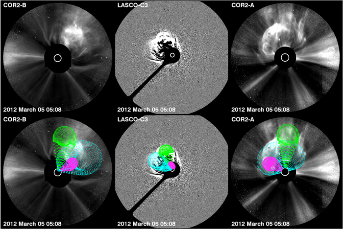
Figure 6. Interaction of CME-3 (blue) with CME-1 (magenta) and CME-2 (green) at 6.8, 13.4, and 13.1 R⊙, respectively. The separate fronts of all three CMEs are most evident in the COR2-A (top right).
Download figure:
Standard image High-resolution imageCME-3 is significantly faster than CME-1 and CME-2 and quickly catches up with the other CMEs within the FOV of COR2. CME-3 appears to overtake CME-1, but the CME-1 front remains visible after the passage of CME-3. In contrast, the front of CME-2 is not overtaken by that of CME-3. The front of CME-2 persists in the observations as a separate structure ahead of the CME-3 front. The fronts of all three CMEs are clearly visible in Figure 6.
Due to the interaction with CME-3, CME-2 is deflected from its initial trajectory. From the GCS model fit, CME-2 initially emerges with a trajectory of N35E64. After the interaction with CME-3, CME-2 trajectory becomes N59E64. Thus, the CME–CME interaction caused a 24° deflection north for a total deflection of 40° in latitude for the SR. The GCS fit also indicated that CME-3 is deflected 10° southward within the span of our observations. However, this relatively small deflection is somewhat ambiguous because it is difficult to separate CME-3 from its shock. We found no change in the trajectory of CME-1 throughout our observations.
The interaction of the three CMEs also affects their velocity. In Figure 7, we plot the 3D HT data from the GCS model for CME-1 (magenta square), CME-2 (green hexagon), and CME-3 (blue triangle). The errors on the heights are derived from multiple fittings of the GCS model to the data after varying the image processing and contrast. For data points shown without error bars, the errors are approximately the size of the plotted symbols. For CME-1, we fit the HT data with an exponential function with three free parameters,

where H is the height and T is the time to estimate the final velocity. The velocities for CME-2 and CME-3 are derived from linear fits to these HT data. The errors of the velocities are the standard uncertainty in the slope of the line (Bevington & Robinson 2003). We found that the HT data for CME-2 are best fit by two linear functions.
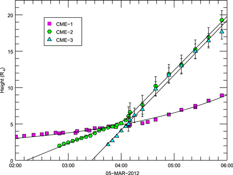
Figure 7. HT plot for CME-1 (magenta squares), CME-2 (green hexagons), and CME-3 (blue triangles) based on the GCS fits and the functions fitted to the data (black). The errors on the heights are derived from multiple fitting of the GCS model to the data after varying the image processing and contrast. For the data points shown without error bars, the errors are approximately the size of the plotted symbols.
Download figure:
Standard image High-resolution imageFrom the HT measurements, the velocity of CME-1 appears to be unaffected by CME-3 or its shock. The velocity of CME-1 smoothly increases with no abrupt acceleration or change in the velocity and is well fit with the exponential function. CME-1 accelerates slowly from an initial average speed of 100 km s−1 to a final speed in the COR2 FOV of ∼550 km s−1 at 10 R⊙. It is possible that the interaction with CME-3 and its driven global shock produced a small increase in the acceleration of CME-1. However, the velocity profile of CME-1 is similar to other streamer blowout type events (Robbrecht et al. 2009). Thus, any change in the CME-1 velocity due to the CME–CME interaction is ambiguous.
In contrast, the interaction of CME-2 and CME-3 is evident in the HT plot. CME-2 emerges with a constant velocity of 576[±28] km s−1 and maintains this velocity until approximately 04:10 UT. As CME-2 and CME-3 interact, CME-2 quickly accelerates to the same velocity as CME-3. The abrupt change in the velocity of CME-2 can best be explained by CME-3 driving CME-2. However, as previously noted, CME-2 does not merge with, nor is it overtaken by, CME-3, and it is fitted as a separate feature in the observations even after the velocity of the two CMEs has coupled. CME-3 maintains a constant velocity of 1456[±31] km s−1 for the entire range of heights.
In addition to the white-light emission examined in this study, CME-3 was also accompanied by intense Type IV, III, and II radio emissions. In particular, the event was marked by a very long-lasting interplanetary Type II burst detected by STA, STB, and Wind. These radio emissions were studied by Magdalenić et al. (2014). However, since Magdalenić et al. (2014) did not study CME-1 and CME-2, they did not discuss any implications from CME–CME interaction associated with the radio emission. It is seems likely that the very intense drifting Type IV continuum detected from 2012 March 5 03:34 UT onward, and intensified after about 4:20 UT, could be associated with the interaction of CME-2 and CME-3 (Figure 7). Similar signatures were seen in past events where CME–CME interaction was observed (Gopalswamy et al. 2001). Finally, contrary to the conclusions in Magdalenić et al. (2014), our results suggest that the interplanetary Type II emission is generated at or close to the CME-3 nose and is therefore originating at a driven shock. This configuration offers a better explanation for the strength of the decametric emission observed by STB.
The difference in the interaction of CME-1 and CME-2 with CME-3 is likely the result of their relative positions. From the GCS fitting, the magnetic structures of CME-2 and CME-3 directly impact, which is expected given that they originate from the same SR. However, for CME-1 and CME-3, it appears that the magnetic structures of these two CMEs do not interact strongly. This weak interaction is also not surprising given that CME-1 and CME-2 did not interact. However, given the size and global influence of the shock driven by CME-3, it is clear from the observations that the shock passed through CME-1. However, the interaction with the shock has little or no effect on the geometry, trajectory, or velocity of CME-1.
4. OBSERVATIONS AT EARTH
The interaction of the three CMEs takes place within the FOV of the coronagraphs. After this interaction, the fronts produced by CME-1 and CME-3 are observed through the SECCHI HI FOVs to Earth from both the STA and STB viewpoints. However, given the large separation of the two STEREO spacecraft from the Sun–Earth line at this time, there are large errors associated with measuring the 3D heights in the HI observations. (See Colaninno et al. (2013) for a discussion of the error with respect to spacecraft separation in the HI observations.) Thus, we do not investigate the propagation of the CMEs outside of the FOVs of the coronagraphs. Möstl et al. (2014) analyzed the heliospheric propagation and arrival time at Earth of CME-3 from a single viewpoint.
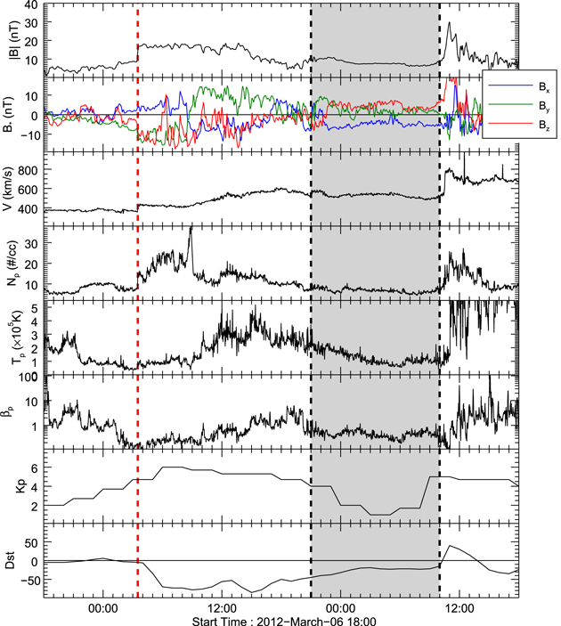
From the HI observations and Möstl et al. (2014), we estimate the arrival of the shock at Earth early on 2012 March 07. Given the trajectory and orientation of CME-3, we expect the shock front and not the magnetic structure of CME-3 to impact Earth. If the magnetic structure of CME-3 did impact Earth, it would be a glancing blow. Figure 8 shows the in situ observations from the WIND (Ogilvie et al. 1995) spacecraft around 2012 March 07. An interplanetary (IP) shock is observed at 03:34 UT on 2012 March 07 characterized by a sharp increase in the magnitude of the magnetic field, plasma velocity, and proton density. There is no clear magnetic cloud or interplanetary CME (ICME) signature following the IP shock. An IP shock and ICME were observed at 11:03 UT on 2012 March 08, which are from a later CME also from AR 11429 after it has rotated closer to the Sun–Earth line. Between these two IP shocks, there is a region of smooth magnetic field that has some rotation in the magnetic field components beginning at 21:00 UT on 2012 March 07 highlighted in Figure 8. This region is a possible ICME; however, the plasma temperature is not not low enough for this classification (I. Richardson 2015, personal communication). The separation between this region and the IP shock is larger than expected if the ICME is driving the shock. If we assume that CME-1 maintains a constant velocity of ∼600 km s−1 after 10 R⊙, then the arrival time of this structure is consistent with CME-1 arriving at Earth. Based on our analysis, we postulate that this region is the magnetic structure of CME-1 and that the lack of low coronal temperatures in the plasma is a result of the shock passing through the flux rope and heating the plasma. This explanation matches our analysis of the observations of the CME-1 and shock in the corona. However, another explanation for this region is a buildup of the solar wind plasma ahead of the 2012 March 08 shock.
Figure 8. Magnetic field and plasma parameters from the WIND spacecraft for the impact of the events at Earth. The geomagnetic parameters (bottom panels) are from the OMNIWeb Plus database. The IP shock (red dashed line) is observed at 03:34 UT on 2012 March 07. The region of smooth, rotating, magnetic field (gray) begins at 21:00 UT on 2012 March 07 before the second IP shock generated by another CME.
Download figure:
Standard image High-resolution image
The bottom two panels of Figure 8 are the geomagnetic parameters Dst and Kp from the OMNIWeb Plus6 database. On 2012 March 05, after the eruption of CME-3, the NOAA Space Weather Prediction Center (SWPC) issued a warning for an expected K-index of 4, no geomagnetic storm. However, the IP shock generated by CME-3 caused a G-2 Moderate geomagnetic storm. On 2012 March 07, Kp = 6 was reached for 3 hr and the Dst reached a minimum of −85 at 15:00 UT. Thus, this event was more geo-effective than predicted.
5. DISCUSSIONS AND SUMMARY
We examine a diverse set of three CMEs and their varied interactions observed simultaneously in the corona at heights below 20 R⊙ from multiple viewpoints. To determine the source, trajectory, geometry, and kinematics of these CMEs before and after their interactions, we used the GCS model to fit the observations from all the data from the six coronagraphs. From our analysis, we find that CME-1 is a slow-rising gradual event originating from north of the Sun–Earth line. The eruption of CME-1 is associated with a prominence eruption with no SXR flare. CME-2 is a moderate impulsive event from an AR that produces a ∼M-class SXR flare. CME-2 has a moderate width of 46° and initial constant velocity of 576[±28] km s−1. CME-3 is a large impulsive event with an X-class SXR flare, a constant velocity of 1456[±31] km s−1, and drives a shock that has a global effect on the corona that is observed as a halo from all viewpoints. The interactions of CME-1 and CME-2 with CME-3 are also remarkably varied.
We find that CME-3 interacts with the preceding CMEs in two ways.
- 1.The CME-3 shock passes through CME-1. It does not seem to alter the CME-1 propagation, nor do we expect it to do so, given that the magnetic structure of the CME has a higher energy density (magnetic, kinetic) compared to the shock. MHD simulations (Lugaz et al. 2005; Xiong et al. 2007) predict that the shock will heat the CME-1 plasma and emerge stronger into the heliosphere. We surmise that this interaction may contribute to both the geo-effectiveness of the shock at Earth and the elevated temperatures in the structure following the shock, which may be CME-1 itself. It would be interesting to test this suggestion with a more detailed analysis of the in situ data or MHD simulation, but this is beyond the scope of this paper.
- 2.The CME-3 deflects CME-2 northward by ∼24° and accelerates it (Figure 7) to basically the same speed as CME-3, more than doubling its initial velocity. This is intriguing because it suggests that the kinetic energy of the system may have increased as a result of the interaction. Such "superelastic" collisions are rarely reported. Shen et al. (2012) is the only other example we are aware of, but their event occurred much farther out in the inner heliosphere (>40 R⊙) with slower events. At such distances, the expected energy increases are quite small and subject to uncertainties. Shen et al. (2012) estimated a 6% kinetic energy increase due to the collision. In our case, the interaction happens at ∼5 R⊙ and involves velocities >1000 km s−s. This result implies that a large energy exchange took place. Whether this is a superelastic collision or not, the momentum exchange should extract a significant amount of energy from CME-3, causing it to decelerate. Indeed, Möstl et al. (2014) report a velocity of 1347 km s−1 for CME-3 in the inner heliosphere. The GCS fits (Figures 5–6) show that the western flank of CME-3 interacts with CME-1 from about 4:00 UT onward, so it could impart some momentum onto CME-1. The lack of observed deflection of CME-1 is consistent with a possible weak acceleration and suggests that the interaction between those two CMEs was weak. Overall, our kinematics support a scenario where CME-3 deflects CME-2 and accelerates CME-2 while losing kinetic energy in the process.
We believe that this work demonstrates both the capability and utility of fitting all CMEs simultaneously even if only one CME is being analyzed. A comparison of our results to a recent publication from Magdalenić et al. (2014) strengthens our assertions. They analyzed the same period, 2012 March 5, but were only interested in the interplanetary evolution of the shock driven by CME-3. Thus, they applied the GCS fit only to what they interpret as CME-3, obtaining a very different size and orientation (see their Figure 3). This discrepancy is not surprising. Since they recognized that CME-2 was in progress but failed to identify CME-1, they would attribute any fitting discrepancies to the overlapping effects from the other CME. We would have done the same thing and probably would have obtained a similar fit if we did not consider a self-consistent fit for all three CMEs. Unfortunately, the possibility of an erroneous GCS fit puts some of their subsequent analysis in doubt. Given the importance of reliable CME orientations and directions for space weather purposes, we emphasize strongly that the fitting of multiple events simultaneously needs to be performed in all cases, even when the researcher is interested in just a single event.
In summary, we have performed the 3D reconstruction of three CMEs simultaneously. This is the first time, to our knowledge, that such a complex 3D reconstruction has been performed using forward modeling methods. The overlapping CMEs present significant challenges for the reconstruction. The outlines of individual CMEs are hard to discern in any given perspective and require the simultaneous analysis of all available observations from all available viewpoints. In addition, the CMEs are not consistently bright in all perspectives since Thomson scatter efficiency can vary significantly for each viewing angle, e.g., CME-1 observed by LASCO (Figure 3). To overcome these difficulties, we spent significant time viewing individual and contemporaneous observations in EUV and white-light to familiarize ourselves with the appearance and timeline of the activity from each viewpoint before attempting the GCS fits. We also verified that the fits are consistent with the observed white-light signatures and the overall coronal morphology for a variety of image processing methods, e.g., running difference, base difference, and background subtraction. In the end, we are satisfied that we can discriminate and fit all three structures to obtain very consistent kinematic results. We identify several interesting results from the observed CME–CME interactions.
- 1.The shock driven by CME-3 passes through CME-1 without any observable changes in the geometry and trajectory of CME-1.
- 2.A possible signature of CME-1 in situ indicates that the CME plasma may have been heated by the passage of the shock.
- 3.CME-2 is accelerated by CME-3 to the same speed, indicating the possibility of a superelastic collision. In the process, CME-3 loses energy and decelerates.
- 4.CME-2 is deflected 24° northward by CME-3 for a total northward deflection of 40° relative to its SR.
- 5.CME-3 interacts with both CME-1 and CME-2, but the fronts of all three CMEs are maintained in the observations. We see no evidence of "cannibalism."
- 6.We demonstrate that the simultaneous fitting of overlapping CMEs is possible, with considerable care, and provides better, more reliable measurements for the individual events compared to fitting a single CME in isolation.
The shock of CME-3 was observed in situ at Earth and produced a G-2 Moderate geomagnetic storm on 2012 March 07. Although the CME–CME interactions did not cause any of the CMEs to become geo-effective (the magnetic structure of CME-3 missed Earth), the propagation and energy changes we deduced suggest that such interactions can have profound implications for space weather predictions, such as significant changes in trajectory and velocity.
These three CMEs produced a complex series of coronal observations with interactions and projection effects that are impossible to analyze without multiple viewpoints. Using both the Earth and STEREO viewpoints, we predicted and explained the Earth impact of these CMEs. Our results show that CME–CME interactions are very sensitive to the 3D location of the CMEs' magnetic structure with respect to each other. To accurately observe and predict the Earth impact of these differences in the CME–CME interactions, an off-axis observation is essential (e.g., from the Lagrangian points; Vourlidas 2015). Also, these CMEs interacted low in the corona, demonstrating the need for a full coverage of observations from the solar surface to Earth from multiple viewpoints.
The SECCHI data are produced by an international consortium of the NRL, LMSAL, and NASA GSFC (USA), RAL and U. Bham (UK), MPS (Germany), CSL (Belgium), and IOTA and IAS (France). The SOHO/LASCO data used here are produced by a consortium of the Naval Research Laboratory (USA), Max-Planck-Institut für Aeronomie (Germany), Laboratoire d'Astronomie (France), and the University of Birmingham (UK). SOHO is a project of international cooperation between ESA and NASA. The AIA data are courtesy of SDO (NASA) and the AIA consortium. This work was supported by NASA and CNR.
Footnotes
- 3
- 4
- 5
- 6