


ABSTRACT
In a recent paper, Kim et al. put forth a steady-state model for the solar wind electrons. The model assumed local equilibrium between the halo electrons, characterized by an intermediate energy range, and the whistler-range fluctuations. The basic wave–particle interaction is assumed to be the cyclotron resonance. Similarly, it was assumed that a dynamical steady state is established between the highly energetic superhalo electrons and high-frequency Langmuir fluctuations. Comparisons with the measured solar wind electron velocity distribution function (VDF) during quiet times were also made, and reasonable agreements were obtained. In such a model, however, only the steady-state solution for the Fokker–Planck type of electron particle kinetic equation was considered. The present paper complements the previous analysis by considering both the steady-state particle and wave kinetic equations. It is shown that the model halo and superhalo electron VDFs, as well as the assumed wave intensity spectra for the whistler and Langmuir fluctuations, approximately satisfy the quasi-linear wave kinetic equations in an approximate sense, thus further validating the local equilibrium model constructed in the paper by Kim et al.
Export citation and abstract BibTeX RIS
1. INTRODUCTION
The solar wind electrons have been detected in situ since the early days of space exploration. It is now well known that the solar wind electrons are made of three or four distinct components. The quasi-isotropic Maxwellian core electrons are the dominant component in terms of the number density, taking up to 96% of the total electron content. The core electrons possess low thermal energy, however, as their typical energy range is characterized by  –103 eV. The next dominant component is the largely isotropic halo component, which may take up to about 4%–5% in number density. The halo component has a net drift with respect to the core component and thus carries the net electron heat flux, which is considered to be important for maintaining the steady-state solar wind structure. The halo electrons possess higher thermal energies when compared with the dense core. Their thermal energy is in the range of 1 to hundreds of keV. The third component is the anti-sunward and highly field-aligned strahl that is generally in the same energy range as the halo, except that their velocity distribution function (VDF) shows a highly anisotropic feature. The fourth component is known as the superhalo, which is present in all solar wind conditions and is highly energetic (tens to several hundreds of keV) and highly isotropic. For historical and recent overviews of studies on solar wind electrons, see, e.g., Montgomery et al. (1968), Vasyliunas (1968), Lin (1973, 1998), Feldman et al. (1975), Rosenbauer et al. (1977), Pilipp et al. (1987a, 1987b), McComas et al. (1992), Lin et al. (1995), Hammond et al. (1996), Fitzenreiter et al. (1998), Maksimovic et al. (2000, 2005), Gosling et al. (2001), Salem et al. (2003a, 2003b), Štverák et al. (2009), and Wang et al. (2012).
Various attempts have been made to model the above-mentioned disparate features associated with the solar wind electrons. Some theories employ collisional dynamics and a phase-space mapping technique to explain the origin and formation of core plus suprathermal features (Scudder & Olbert 1979a, 1979b; Scudder 1992, 1994; Canullo et al. 1996; Lie-Svendsen et al. 1997; Pierrard et al. 1999, 2001; Lie-Svendsen & Leer 2000; Landi et al. 2012). The collisional effects are generally important for low corona, near ∼10  or below, where
  is the solar radius, but for higher altitudes, and especially near 1 AU, the collisional effects are generally unimportant. Even for low altitudes, high-energy electrons such as the halo and superhalo populations are not significantly influenced by the binary Coulomb collisions. In this respect, the wave–particle resonant interaction and the collective dissipation are important, and such an effect has also been considered together with other global features associated with the solar wind (Vocks & Mann 2003; Vocks et al. 2005; Pierrard et al. 2011; Pavan et al. 2013; Yoon 2014). The most general models of the solar wind electrons must include not only the collisional dynamics and wave–particle resonance effects but also other effects such as the large-scale density and magnetic field inhomogeneities, as well as large-scale electric field.
In a recent paper, Kim et al. (2015) specifically focused on the details associated with the wave–particle interaction while ignoring other large-scale effects. These authors gave careful considerations to the issue of whether certain self-generated plasma fluctuations are capable of maintaining the specific velocity-space spectral profiles associated with the solar wind electron distribution functions. Since Kim et al. (2015) assumed quasi-isotropic VDFs for the halo and superhalo electrons and ignored any possible relative drifts associated with these components, the source of plasma fluctuations had to be the spontaneous emission, since no instability operates for isotropic VDFs without drifts. Consequently, they included the effects of discrete particles and thermal spontaneous emissions. Their analysis, however, assumed the preexistence of energetic solar wind electrons and did not address the question of the origin of these electrons. Instead, their concern was whether certain plasma waves can be self-generated by these electrons via spontaneous emissions, which can in turn interact with the electrons in order to maintain the steady-state electron distribution function.
Kim et al. (2015) put forth a model in which the highly energetic superhalo component maintains a steady-state wave–particle resonance with the high-frequency electrostatic fluctuations pervasively observed in the solar wind, which is known in the literature as the quasi-thermal noise (Meyer-Vernet 1979; Meyer-Vernet & Perche 1989; Lund et al. 1996; Lazar et al. 2012; Schlickeiser & Yoon 2012; Felten et al. 2013; Yoon 2014). The quasi-thermal noise spectrum is characterized by a  frequency range, which can be shown to satisfy the Landau wave–particle resonance condition,
  with the superhalo electrons. On the other hand, for the halo electrons, the appropriate plasma wave is the whistler fluctuations with the frequency range
  This type of wave can be shown to be in cyclotron resonance,
  with the electrons whose energy range lies within those that typify halo electron thermal energy. The existence of whistler fluctuations is not as straightforward to verify observationally, but a recent paper by Lacombe et al. (2014) may be an exemplary case. Their paper analyzed the Cluster data and demonstrated several clear examples of quasi-parallel, right-hand circularly polarized whistler waves with the frequency range, which is about 1/10 that of the local cyclotron frequency. As Lacombe et al. (2014) note, the unambiguous identification of whistler fluctuations is not always easy, owing to the occultation by the Doppler-shifted solar wind turbulence, which may be intrinsically low frequency, but nevertheless may appear to be high frequency owing to the solar wind motion past the spacecraft.
Motivated by findings by Lacombe et al. (2014), Kim et al. (2015) formulated a steady-state theory for the solar wind electron distribution by solving the Fokker–Planck type of electron kinetic equation in which the velocity-space friction coefficient is computed from the theory of spontaneous emission while the velocity-space diffusion coefficient is calculated from the standard quasi-linear theory. By balancing the friction and diffusion terms, they obtained the steady-state VDFs for halo and superhalo electron components. They also made comparisons between the theoretical models and the actually measured solar wind electron VDF, which was obtained during the quiet-time solar wind conditions by STEREO A and B spacecraft. Kim et al. (2015) obtained good agreements between the models and the data.
Despite the overall favorable comparisons between the theory and observation, however, the question of whether the wave spectra that were used as inputs for the computations of halo and superhalo electron distributions also satisfy the steady-state wave kinetic equation was not directly addressed in Kim et al. (2015). Unlike the particle kinetic equation, the wave kinetic equation encompasses generally linear wave–particle resonant interactions, as well as nonlinear wave–wave resonance and nonlinear wave–particle interaction. Solutions to the steady-state wave kinetic equation must balance the various linear and nonlinear terms, which is quite challenging. The purpose of the present paper is to consider the self-consistency associated with the steady-state wave kinetic equation for both the Langmuir and whistler waves, but for the sake of simplicity, the analysis is restricted to the linear wave–particle resonant interactions. In spite of such a simplification, however, the present analysis constitutes a crucial step that further establishes the theoretical foundation for the models of solar wind electrons.
2. OVERVIEW OF THE STEADY-STATE SOLAR WIND ELECTRON MODEL
To briefly overview the theory by Kim et al. (2015), the steady-state solution to the electron kinetic equation was obtained by assuming that the velocity-space friction term  and the velocity-space diffusion term
  cancel each other out, thereby maintaining the stationary state. Here we repeat the particle kinetic equation considered by Kim et al. (2015),
where fa is the one-particle VDF for species a, where a = h refers to the halo electrons, a = s denotes the superhalo component, and the velocity friction coefficient  and the diffusion coefficient
  in a cylindrical coordinate system are given by
and
In Kim et al. (2015), we determined the velocity friction coefficient by considering the residue contributions from the eigenmodes only,
where  and
and  are Langmuir and whistler wave dispersion relations, respectively, which satisfy the dispersion relations,
  and
and  respectively. Hence, for these eigenmodes, the denominators are expanded in Taylor series as

 and
and 


 respectively. The imaginary part thus comes from the residues. This procedure is equivalent to taking only the spontaneously emitted Langmuir and whistler waves as the source of velocity-space friction. Ma & Summers (1998), on the other hand, made use of the velocity friction coefficient that arises purely from the binary collisions. Within the context of the above consideration, this is equivalent to assuming that the most important contribution to the velocity friction arises from the non-eigenmodes, or those ω and k that do not satisfy the dispersion relations,
  and
and  Such an assumption would lead to the velocity-space friction from collisional processes, which is equivalent to the treatment by Ma & Summers (1998). In Kim et al. (2015), such a non-eigenmode contribution was ignored. For a general case, both the eigenmodes and non-eigenmodes should contribute to the velocity-space friction. However, such a general treatment has not been done hitherto.
Upon assuming the steady-sate  averaging over the velocity-space pitching angle, and balancing the friction and diffusion terms, Kim et al. (2015) derived the halo electron steady-state VDF,
where C is the normalization constant, me and c present the electron mass and the speed of light in vacuo, respectively. The quantity km2 is the longest possible perpendicular wavelength associated with the spontaneously emitted whistler wave fluctuation, which can be taken to be on the order of inverse thermal electron gyroradius,  Here
Here  is the square of the electron cyclotron frequency, e and B0 being the unit electric charge and the intensity of the ambient magnetic field, respectively, and
  is the square of the thermal speed associated with the Maxwellian core electrons, T0 being the core electron temperature (defined in units of energy, i.e., eV). The quantity
  is the square of the plasma oscillation frequency, ne being the total electron number density. In Equation (1), μ is the cosine of the velocity pitch angle, and the quantities Ah and Dh are related to the friction and diffusion coefficients. The quantity
  denotes the square of the spectral electric field amplitudes associated with the whistler waves, which is the same as the spectral electric field wave energy density apart from the
  factor.
Kim et al. (2015) likewise constructed the steady-state VDF for the superhalo electrons,
where  represents the same spectral electric field wave energy density associated with the Langmuir waves (apart from the same
  factor).
As the formal solutions (1) and (2) indicate, the specific mathematical form of the electron VDFs depends on the functional form of the wave spectra that enter the diffusion coefficient. Kim et al. (2015) constructed the solution by making judicious choices of the wave spectra for both whistler and Langmuir fluctuations. For the whistler wave spectrum Kim et al. (2015) noted that typical solar wind turbulence in the whistler frequency range exhibits an inverse power-law behavior. Consequently, they modeled the wave spectrum by (see Equation (42) of Kim et al. 2015)
where α is treated as a free adjustable parameter. Note that  corresponds to the thermal whistler wave fluctuation. The reason for the above choice was based on observations of the typical solar wind turbulence spectrum in the whistler frequency range, which shows the inverse power-law spectrum in frequency space. Upon inserting Equation (3) into formal solution (1), Kim et al. (2015) found that the normalized halo electron distribution is given by (see Equation (46) of Kim et al. 2015)
where the normalization is according to  where nh is the halo electron number density. In the above
  is the gamma function, and vTh is the effective thermal speed for the halo electrons. As a corollary to solution (4), Kim et al. (2015) also determined the specific expression for the constant
  which is consistent with the particle distribution. The specific form of the model whistler wave spectral function is thus given by
Note that the quantity Hα in the above is treated as an undetermined parameter. Comparison of the model given by Equation (4) and the measured electron VDF produced a rather good fit, as shown in Figure 2 of Kim et al. (2015). To recapitulate their model, they assumed that the density ratio of the core-to-total electrons is given by  core thermal speed is
  halo-to-total electron density ratio is
  and the ratio of core thermal speed to halo thermal speed is
  The spectral index of
  was also adopted. Note that the whistler spectrum of inverse power law in wave number or frequency is consistent with the typical observation.
Kim et al. (2015) also considered an alternative model for the halo VDF, namely, the kappa (or Lorentzian) distribution. The reason is because such an empirical model is often employed in the literature (e.g., Wang et al. 2012). Kim et al. (2015) then posed the question of what type of whistler wave spectrum would produce the Lorentzian model for the halo component, regardless of whether it is supported by observation or not. It turns out that the model spectrum of the form (see Equation (50) of Kim et al. 2015)

can be shown to be consistent with the Lorentzian model. Observational justification of the above model is not so clear. It is fair to say that the above model is necessary in order to generate the desired Lorentzian halo electron VDF. To reiterate, whether the whistler spectrum of the form given by Equation (6) is consistent with observation of turbulence spectra in the solar wind is not of pertinence here. It is simply a necessary condition for the Lorentzian (or kappa) model of the halo electron VDF. In any event, the alternative Lorentzian VDF can be derived upon inserting Equation (6) into Equation (1),
as well as the whistler wave spectrum with the coefficient  and the parameter
  determined properly from Equation (2),
where H1 is the same as Hα defined in Equation (5), except  Again, the quantity H1 is treated as an undetermined parameter. For the alternative model Kim et al. (2015) assumed
  and
and  Other dimensionless parameters were the same as the first model. Comparison between the alternative halo model and the actual data can be found in Figure 3 of Kim et al. (2015), which demonstrates that the Lorentzian model provides a marginally improved comparison with the observation.
Finally, we overview the superhalo electron model and the Langmuir turbulence spectrum that leads to the electron distribution. Modeling the Langmuir wave spectrum was based on a more firm theoretical foundation. Kim et al. (2015) simply followed an earlier work by Yoon (2014), who theoretically constructed the so-called turbulent equilibrium solution between the kappa distribution of electrons and Langmuir turbulence spectrum on the basis of kinetic weak turbulence theory for unmagnetized plasmas, where Yoon (2014) showed that the Langmuir wave spectrum of the form (see Equation (29) of Kim et al. 2015)
uniquely satisfies the balance of spontaneous and induced emission terms, as well as the balance of spontaneous and induced scattering terms in the wave kinetic equation. Note that the above form of the Langmuir wave spectrum is also consistent with the quasi-thermal noise spectrum, and that it is consistent with observations (Yoon 2014). Guided by such a finding, Kim et al. (2015) adopted the same model and obtained the steady-state superhalo electron VDF, as well as the coefficients  and
and  , so that the net solution is given by
Here vT0 represents the thermal speed of the Maxwellian core electrons, while vTs denotes the effective thermal speed for the superhalo electrons. The reason vT0 determines the level of Langmuir fluctuations is that the Langmuir wave is a thermal plasma wave, whose dispersive property is largely determined by the dense but low-energy core electrons. In Kim et al. (2015), the superhalo kappa index of  was adopted, following the theoretical prediction by Yoon (2014), who not only showed that the electron kappa VDF is a turbulent equilibrium but also computed the kappa index. According to observations, the superhalo electron density is generally extremely low, so that Kim et al. (2015) chose
  The superhalo thermal speed, on the other hand, is very high when compared with the core thermal speed. Accordingly, Kim et al. (2015) adopted
To recap the findings in Kim et al. (2015), model spectra (3), (6), and (9), respectively, were adopted in order to construct the electron VDFs (4), (7), and (10), in that order. Such a modeling of the solar wind electrons was entirely based on the consideration of the particle kinetic equation. However, they did not ask the question whether the wave spectra also satisfy the wave kinetic equation or not. Since the particle kinetic equation and quasi-linear wave kinetic equation are both dictated by the same linear wave–particle resonance conditions, intuitively one may expect that the model wave spectra should also satisfy the quasi-linear portion of the wave kinetic equation, if not necessarily the nonlinear part of the wave kinetic equation. However, one must show that such an assumption is valid. In the present paper, we consider the reverse problem. That is, we now use model electron VDFs (4), (7), and (10), respectively, in the wave kinetic equation and determine whether indeed we obtain the model wave spectra (3), (6), and (9). As will be shown, the model wave spectra can be reconciled with the particle kinetic equation under a heuristic approximation. Thus, the answer to the question of whether the model electron VDFs (4), (7), and (10) lead to the model wave spectra (3), (6), and (9), respectively, is a qualified "yes."
We also discuss exact mathematical conditions for exact and rigorous solutions. However, we find that the general exact solution is not forthcoming at the present moment. Instead, we discuss a couple of limiting solutions. Apart from the exact solutions, numerical comparisons demonstrate that the heuristic solutions are sufficiently accurate such that the models of the solar wind electrons discussed by Kim et al. (2015) are approximately valid and may represent a practically self-consistent solution. In what follows, we discuss these findings in detail.
3. THE STEADY-STATE WAVE INTENSITY
We start from the wave kinetic equation in the linear approximation for a plasma immersed in a constant magnetic field (Gaelzer et al. 2015),
The first equation describes the time evolution of the longitudinal waves propagating in parallel direction with respect to the ambient magnetic field, while the second equation depicts the dynamic evolution of the two circularly polarized transverse waves propagating in parallel direction, ± signs denoting the right/left-hand circular polarization. The terms on the right-hand side arise from the discrete particle effects, i.e., thermal spontaneous emission of EM fluctuations. In the above k represents the parallel component of the wave vector. We already encountered the quantity km2 associated with the spontaneous emission terms. This quantity is the result of integration of spontaneous emission terms in perpendicular wave number space where the upper limit was replaced by the cutoff,  The reason for the
  integration was first noted by Gaelzer et al. (2015), who pointed out that even though the plasma eigenmodes (such as Langmuir and whistler waves) can be treated as quasi-parallel modes, the spontaneously emitted fluctuations should not have any intrinsic directionality since they are generated by random thermal motions of the plasma particles. Hence, the quasi-parallel formalism of the plasma kinetic theory requires the integration over
  space. The upper limit km was determined by Gaelzer et al. (2015) on the basis of the approximation that the argument of the Bessel function be small,
  and thus
  The specific value of km is unimportant, however.
In Equation (11), the longitudinal and transverse dielectric constants are respectively given by
3.1. Steady-state Whistler Fluctuation Spectral Intensity
We are interested in the steady-state wave kinetic equation. Let us consider the transverse whistler wave branch (+ sign),
From Equation (12) we have
Making use of the whistler wave properties for the low-frequency regime,  (Kim et al. 2015), namely,
we may rewrite Equation (13) as
Since we consider low frequency,  we may approximate the resonance condition by ignoring
  in comparison with
![$\delta \left[{\omega }_{{\rm{W}}}(k)-{{kv}}_{\parallel }-| {{\rm{\Omega }}}_{e}| \right]\approx \delta ({{kv}}_{\parallel }+| {{\rm{\Omega }}}_{e}| ).$](https://content.cld.iop.org/journals/0004-637X/812/2/169/revision1/apj520296ieqn62.gif) Upon rewriting (16) in a velocity-space spherical coordinate system and making use of the fact that fe is isotropic, we have
Upon rewriting (16) in a velocity-space spherical coordinate system and making use of the fact that fe is isotropic, we have
In the above,  is the cosine of the velocity pitch angle. We have made use of the fact that the velocity integral can be expressed as
  We may now make use of Equation (17) to test the validity of the wave intensity spectra for the whistler waves adopted by Kim et al. (2015). This can be done by substituting the model VDF (4) or alternatively (7) into Equation (17) and seeing whether the wave intensity computed on the basis of Equation (17) is indeed consistent with Equation (5) or the alternate model (8).
3.1.1. Halo Electron Model 1
First, consider the halo electron model 1, which is given by Equation (4). Upon inserting the model VDF (4) into Equation (17) and carrying out the v integration by virtue of the delta function, we find, after some straightforward manipulations and restricting ourselves to  without loss of generality, that the result is the following:
At this point, the wave spectrum  can be determined by equating the right-hand side to zero, but in doing so, one must integrate over the exponential factor. However, it becomes evident that doing so will lead to a result that is not entirely identical to Equation (5), since Equation (5) does not have any factor with the exponential factor, whereas Equation (18) does. This already shows that Equation (5) is an approximation. The question is how good the approximation is? We will compare Equation (5) and the rigorous
  determined from Equation (18) that includes the μ integral, but for now, we take a heuristic approach. We first note that the necessary condition for the equality in Equation (18) is that the integrand identically vanish,
Of course, this is not always guaranteed since the above equality must be satisfied for all μ and all k, but let us assume the above condition for now. In order to recover the model spectrum (5), we simply multiply the factor  and integrate over μ from 0 to 1. This leads to
The resulting expression for  is identical to Equation (5). Of course, this is a heuristic treatment.
On the other hand, if we do not set the integrand to zero arbitrarily as in Equation (19), but instead solve for  directly from Equation (18), then one can show that the resulting spectrum is the same as Equation (5) in its overall functional form, except that the factor HW should be replaced by
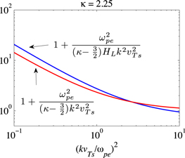
Note that  is no longer a constant, but is a function of k. In Figure 1 we plot the two quantities defined by
respectively, versus  in log–log plot format, for
  Figure 1 shows that the above two quantities are qualitatively similar, which indicates that the model adopted in Kim et al. (2015) is indeed consistent with the quasi-linear wave kinetic equation, at least in an approximate sense.

Figure 1. Comparison between the model spectrum (5) defined in terms of the form factor HW, which resulted as a corollary of the steady-state particle kinetic Equation (1), vs. the whistler wave spectrum defined with the form factor  which was deduced from the steady-state wave kinetic Equation (18). Note that the two form factors lead to qualitatively similar results.
Download figure:
Standard image High-resolution image3.1.2. Halo Electron Model 2
Next, we consider the halo electron model 2, which is the Lorentzian (or kappa) distribution function (7). This is an alternative model of the halo VDF. Inserting model (7) into the steady-state whistler wave kinetic Equation (17), we obtain the equation for the alternative whistler spectrum,
Again, to determine ![${[{E}_{{\rm{W}}}^{2}]}_{({\rm{alt}})}(k)$](https://content.cld.iop.org/journals/0004-637X/812/2/169/revision1/apj520296ieqn75.gif) rigorously from the above, one must integrate over μ including the Lorentzian factor
rigorously from the above, one must integrate over μ including the Lorentzian factor  As with Equation (18), doing so leads to a result, which is not exactly consistent with Equation (8). We thus approach the problem first, heuristically, by writing down the necessary condition for the equality in Equation (23),
By multiplying the factor  and integrating over μ from 0 to 1, we arrive at
The solution to the above equation is, of course, identical to Equation (8). In other words, if we take the liberty of isolating the integrand of Equation (23) and setting it equal to zero, then we may manipulate the necessary condition (24) by multiplying the form factor and integrating over μ in order to obtain the convergence between the steady-state wave kinetic equation and the wave spectrum that emerges from the consideration of the particle kinetic equation.
If, on the other hand, we determine ![${[{E}_{{\rm{W}}}^{2}]}_{({\rm{alt}})}(k)$](https://content.cld.iop.org/journals/0004-637X/812/2/169/revision1/apj520296ieqn78.gif) directly from Equation (23), then one can show, after some straightforward manipulations, that a slightly different form of the alternative wave spectrum emerges,
directly from Equation (23), then one can show, after some straightforward manipulations, that a slightly different form of the alternative wave spectrum emerges,
Upon comparison with the model spectrum (8), the most notable difference is that the form factor  is now a function of k.
Shown in Figure 2 is the plot of two quantities,
versus  in the same log–log plot format as in Figure 1. Note that the two different form factors lead to qualitatively similar results. Figure 2 thus shows that the alternative halo model works equally well in the approximate sense.
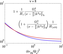
Figure 2. Comparison between the alternative model spectrum (8), defined in terms of the form factor  and the alternative wave spectrum defined with the form factor
  Note that the two form factors lead to qualitatively similar results, albeit when compared with model 1, the convergence is less favorable.
Download figure:
Standard image High-resolution image3.2. Steady-state Langmuir Fluctuation Spectral Intensity
Next, we consider the steady-state wave kinetic equation for Langmuir waves. From the first equation in Equation (11), we write down the steady-state condition,
From the first equation in Equation (12), we have
We make use of the Langmuir wave properties,
This leads to
where we have assumed isotropic fe and approximated  Inserting the superhalo electron kappa VDF into Equation (31), we obtain
From Equation (32), we write down the necessary condition for the equality,
which, upon multiplying μ and integrating over  leads to
Of course, the solution  is identical to Equation (10), thus demonstrating that the consideration of the steady-state wave kinetic equation leads to a heuristic reconciliation with the Langmuir wave spectral intensity that follows from the consideration of the steady-state particle kinetic equation.
If we directly solve for  from Equation (32) leaving the μ integral intact, then one finds, after some straightforward calculations, that the result is virtually identical to Equation (10), except that the form factor HL does not appear within the large parentheses, but it is actually unity. We thus plot in Figure 3 two quantities,
versus  in log–log scale. As the reader may appreciate, the two model spectra exhibit at least a qualitative similarity; hence, the superhalo model adopted in Kim et al. (2015) appears to be validated in an approximate sense.
Figure 3. Comparison between the model Langmuir waves spectrum (10), defined in terms of the form factor HL, and the spectrum deduced directly from the wave Equation (32). Again, the two alternative spectra lead to qualitatively similar results.
Download figure:
Standard image High-resolution image
4. SUMMARY AND DISCUSSION
In Kim et al. (2015), we constructed the solar wind halo and superhalo electron VDFs on the basis of the steady-state particle kinetic equation by assuming model spectra (3), (6), and (9), for the whistler and Langmuir fluctuations. The result was the electron VDFs (4), (7), and (10), respectively, which agreed fairly well with observations made by STEREO and WIND spacecraft. In the present paper we considered the reverse problem. That is, we now use model electron VDFs already constructed in Kim et al. (2015), namely, (4), (7), and (10), respectively, but we addressed the issue of whether we may obtain the model wave spectra (3), (6), and (9) within the context of the steady-state wave kinetic equation. To summarize the findings, we achieved an exact agreement between the model spectra, (5), (8), and (10), and the wave spectra that emerge from consideration of the steady-state wave kinetic equation, namely, (20), (25), and (34), by means of a heuristic argument. That is, if we arbitrarily assume that the integrands of (18), (23), and (32) are zero, then from such an assumption, we may subsequently manipulate the resulting formulae for the wave spectra in order to attain the exact agreement. However, admittedly, such a treatment is approximate and heuristic, since the equality it not necessarily guaranteed for all pitch angles and wave numbers. Consequently, we also solved the wave spectra directly from Equations (18), (23), and (32) by leaving the μ integrals intact. Upon comparing the outcomes of the two approaches, we found some discrepancies, as expected, but also qualitative agreements. From this, we thus concluded that the approximate models of the solar wind electron VDF put forth by Kim et al. (2015) are also consistent with the steady-state quasi-linear wave kinetic equation.
The outstanding question is whether there exists a rigorous mathematical solution for the self-consistent particle and wave solutions. The problem boils down to finding exact solutions for the particle VDF fe(v) and the wave intensity  from the coupled integral equations. In the case of halo electrons, the coupled set of equations for halo electron VDF and whistler wave fluctuation spectral intensity would be
and for the case of superhalo electrons and Langmuir wave fluctuation, it is
where  In dimensionless form Equations (36) and (37) may be expressed by
and
One can show that the Maxwellian VDFs for  and
and  and constant Langmuir fluctuation spectrum,
  and whistler spectrum of the form
  exactly satisfy the coupled Equations (36) and (37). To see this, let us assume that for the superhalo, the dimensionless VDF and Langmuir wave spectrum are given by
  and
and  Then upon inserting these into Equation (39), one finds that thermal equilibrium, expressed in terms of dimensional VDF and Langmuir wave spectrum,

is an exact solution. In the case of the halo model, one also finds from Equation (38) that

is an exact solution.
There is another exact solution, namely, the power-law VDF. For the superhalo, if we assume  and insert this into the second equation in Equation (39), then one finds that
 ![${E}_{{\rm{L}}}^{2}(k)=1/[(b-2){k}^{2}].$](https://content.cld.iop.org/journals/0004-637X/812/2/169/revision1/apj520296ieqn97.gif) Inserting this result into the first equation in Equation (39), one obtains
Inserting this result into the first equation in Equation (39), one obtains  In order to obtain a consistent solution, one must have
  or b = 4. We thus have the exact power-law solution,

The kappa VDF for the superhalo and the associated Langmuir wave spectrum (10), in a way, encompass aspects of both the Maxwellian exact solution (40) and the power-law solution (42) in that for a low velocity range the kappa VDF approaches the Maxwellian model, while for high velocities the kappa model becomes an inverse power law. Note that the kappa VDF (10) asymptotically behaves as  which for
  becomes
  This was shown to be consistent with observation,
  where
where  (Wang et al. 2012). On the other hand, the exact solution (42) predicts that VDF should be
  Perhaps the power-law index 4 is the limiting case. Despite this discrepancy, the fact that the two exact models (40) and (42) are encompassed by the single kappa model (10) is noteworthy.
For the halo, if we assume a power-law VDF  then we have from the wave equation in Equation (38) the wave spectrum of the form
  which, in turn, leads to the VDF from the first equation in Equation (38),
If we formally define

then we have

By equating  , we obtain

Consequently, the exact power-law VDF for the halo electrons and whistler spectrum emerge,

Note that one can write the quantity H in terms of the wave spectrum,
Consequently, the power-law VDF for the halo electrons and the constant whistler wave spectrum that exactly satisfy the linear particle and wave kinetic equation can be written as
Note that the Lorentzian (or kappa) model of the halo electrons (7) is consistent with the exact Maxwellian and power-law solutions (41) and (49) in that the Lorentzian model (7) reduces to the Maxwellian mode for low v, while for high v, the model (7) asymptotically approaches the power-law VDF,  Observation shows that the power-law index of the halo VDF is higher than that of the superhalo. Equation (49) is consistent with such a fact in that the halo power-law VDF is characterized by
  which is always higher than that of the superhalo power-law index, namely, 4. The outstanding question is whether other exact solutions besides the thermal equilibrium and power-law solutions exist. The answer to this question remains unknown.
This work was supported in part by the BK21 plus program through the National Research Foundation (NRF) funded by the Ministry of Education of Korea. P.H.Y. acknowledges NSF grants AGS1138720 and AGS1242331 to the University of Maryland. G.S.C. was supported by the Basic Science Research Program through the National Research Foundation of Korea (NRF) funded by the Ministry of Education (NRF-2013R1A1A2058937).