


ABSTRACT
We investigate the relation between star formation (SF) and black hole accretion luminosities, using a sample of 492 type-2 active galactic nuclei (AGNs) at  , which are detected in the far-infrared (FIR) surveys with AKARI and Herschel. We adopt FIR luminosities at 90 and 100 μm as SF luminosities, assuming the proposed linear proportionality of star formation rate with FIR luminosities. By estimating AGN luminosities from [O iii]λ5007 and [O i]λ6300 emission lines, we find a positive linear trend between FIR and AGN luminosities over a wide dynamical range. This result appears to be inconsistent with the recent reports that low-luminosity AGNs show essentially no correlation between FIR and X-ray luminosities, while the discrepancy is likely due to the Malmquist and sample selection biases. By analyzing the spectral energy distribution, we find that pure-AGN candidates, of which FIR radiation is thought to be AGN-dominated, show significantly low-SF activities. These AGNs hosted by low-SF galaxies are rare in our sample (
 ). However, the low fraction of low-SF AGNs is possibly due to observational limitations since the recent FIR surveys are insufficient to examine the population of high-luminosity AGNs hosted by low-SF galaxies.
Export citation and abstract BibTeX RIS
1. INTRODUCTION
In recent decades the connection between galaxy evolution and the growth of supermassive black holes (SMBHs) has been one of the main topics in extragalactic research. The tight correlation of black hole mass,  , with galaxy properties, e.g., stellar velocity dispersion,
  (e.g., Magorrian et al. 1998; Marconi & Hunt 2003; Woo et al. 2010, 2013), suggests the coevolution of galaxies and SMBHs although the physical link between them has yet to be clearly revealed. Various observational studies have been devoted to investigating the nature of the coevolution. For example, the redshift evolution of the
  –
– relation, representing a cumulative growth history, has been investigated mainly using type-1 active galactic nuclei, (AGNs; e.g., Woo et al. 2006, 2008; Merloni et al. 2010; Schramm & Silverman 2013). The connection between on-going star formation (SF) and AGN activity is also one of the observational signatures, revealing the connection of the growth of stellar mass and the BH growth at the observed epoch (e.g., Sanders et al. 1988; Cid Fernandes et al. 2001; Kauffmann et al. 2003; Netzer 2009; Alexander & Hickox 2012; Rosario et al. 2012).
Various theoretical frameworks have been suggested to explain the AGN-SF link and also reproduce the  –
– relation. For example, based on the smoothed particle hydrodynamic N-body simulations of gaseous galaxy mergers, Blecha et al. (2011) showed simultaneous bursts of SF and BH accretion (see also Hopkins & Quataert 2010). Such theoretical models predict a positive correlation between SF and AGN activity, as consistent with the results of several observational studies (e.g., Netzer et al. 2007; Netzer 2009; Diamond-Stanic & Rieke 2012; Rovilos et al. 2012; Karouzos et al. 2014). Note that other studies reported that there is a time lag between SF and AGN phases (e.g., Davies et al. 2007; Wild et al. 2010; Matsuoka et al. 2011; Cen 2012; Hopkins 2012).
While the AGN-SF link can be investigated in various aspects, the direct comparison between AGN and SF luminosities, i.e., the  –
– relation, is the most simple approach. Since the SF luminosity corresponds to the on-going growth of galaxies and the AGN luminosity reveals the current growth of SMBHs, the AGN-SF connection can be directly traced at the observed epoch. A correlation between SF and AGN luminosities has been reported in previous studies, indicating that luminous AGNs are hosted by highly star-forming galaxies. Based on the combined sample of local type-2 AGNs and quasars at
  , for example, Netzer (2009) found that there is a good correlation between SF and AGN luminosities, albeit with substantial scatters (see also Netzer et al. 2007; Lutz et al. 2008; Woo et al. 2012). Recently, Tommasin et al. (2012) have found a correlation between
  and
and  of low-ionization nuclear emission-line regions (LINERs). These results suggest that BH activity is connected with SF.
Based on the deep Herschel imaging of the X-ray sources at  in the fields of GOODS and COSMOS, Rosario et al. (2012) have reported a correlation between AGN and FIR luminosities. In their study, luminous X-ray AGNs at
  show a correlation between AGN and FIR (i.e., 60 μm) luminosities, as similarly presented by earlier works (e.g., Netzer et al. 2007; Lutz et al. 2008; Netzer 2009) while the correlation flattens or disappears at
  (see also, e.g., Hatziminaoglou et al. 2010; Lutz et al. 2010; Shao et al. 2010; Harrison et al. 2012; Page et al. 2012). In contrast, they claimed that low-luminosity AGNs show essentially no correlation between FIR and AGN luminosities at all redshifts. The enhanced SF for given AGN luminosity of their low-z X-ray AGNs (
 ) seems to be in contrast with the finding of Netzer (2009) that local type-2 AGNs (
 ) show a positive correlation between SF and AGN luminosities. This discrepancy may be caused by observational biases, e.g., the Malmquist and sample selection biases, and from the measurement uncertainties in SF and AGN luminosities. It is also possible that for a given AGN luminosity, galaxies with lower SF luminosities may be undetected due to the FIR flux limit. Therefore, in order to fully reveal the connection between AGN and SF activities it is crucial to examine potential biases, which may affect the
  –
– relation.
FIR luminosity is often used as an SF indicator since the rest-frame FIR emission is mainly from the host galaxy while the AGN contribution to FIR, ∼50−150 μm, is due to the Rayleigh–Jeans tail of an AGN-heated dust component (e.g., Netzer 2009; Mullaney et al. 2012; Rosario et al. 2012). In the case of AGN luminosity, X-ray luminosity can be used with a proper bolometric correction. However, X-ray data with sufficient depth is often not available. Instead, emission lines from the narrow-line regions, e.g., Hβ, [O iii]λ5007, [O i]λ6300, and [O iv]λ25.89 μm lines, are often used as a proxy for AGN bolometric luminosity (e.g., Netzer 2009; Diamond-Stanic & Rieke 2012).
In this paper, we investigate the AGN-SF connection for a sample of type-2 AGNs at  selected from the Sloan Digital Sky Survey (SDSS), using AKARI and Herschel data. In Section 2, we describe the sample selection and the data. Section 3 presents the main results and Section 4 provides discussion and interpretation. The summary and conclusion are given in Section 5. We adopted a concordance cosmology with (
 ,
,  ) = (0.3, 0.7) and
  = 70 km s−1 Mpc−1.
2. SAMPLE AND DATA
In this study, we mainly focus on the local type-2 AGNs selected from SDSS, for which FIR data are available. Using SDSS spectroscopic data and FIR survey data, we investigate the relation between AGN and FIR luminosities in the wide dynamic range. We also collect multi-wavelength data, e.g., ultraviolet (UV) and mid-infrared (MIR), to examine the characteristics of the galaxies in the sample. In this section, we describe our sample selection and multi-wavelength data.
2.1. Type-2 AGN Sample
We selected type-2 AGNs at  from the MPA-JHU SDSS DR7 galaxy catalog,3
including
from the MPA-JHU SDSS DR7 galaxy catalog,3
including  galaxies, based on the BPT diagnostic diagram (e.g., Baldwin et al. 1981) using the [O iii]λ5007/Hβ and [N ii]λ6584/Hα flux ratios with the classification scheme in Kewley et al. (2006). Note that we excluded composite objects since they are unreliable in estimating AGN luminosities from narrow-emission lines due to the contribution from SF. In the selection process, we also adopted the following criteria: a reliable redshift measurement (i.e.,
  ) and high signal-to-noise ratios (S/Ns) for emission lines which were used in AGN classification, i.e.,
  for [O iii]λ5007, Hα, and [N ii]λ6584 lines,
  for the Hβ line. As a result, we obtained 35,945 type-2 AGNs.
Note that our sample contains both Seyfert 2s and LINER 2s, although the physical connection between them is not clear as discussed in various studies. Especially understanding the ionization process of LINERs is essential in our study because it directly relates to the estimate of AGN luminosities (Section 3.2). Mainly, there are three considerations for LINER 2s: (1) hot stars, i.e., post-AGB star and blue stars showing similar line-flux ratios to LINERs, (2) shock ionizations instead of photoionozations, and (3) low-ionization parameters of LINER 2s. In order to consider these issues, we divide our sample into two subsamples, i.e., Seyfert 2s and LINER 2s (Section 2.2). To remove stars showing similar line-flux ratios to LINERs, we identify the so-called [O i]λ6300-weak LINERs, which are considered non-AGNs. By adopting a criterion, i.e., [O i]λ6300/Hα  (e.g., Filippenko & Terlevich 1992; Alonso-Herrero et al. 2000), we exclude LINER 2s (see Section 2.2). Regarding shock ionizations, we expect that shocked gas should lead to higher excitation UV spectra than photoionized gas. Thus, strong UV emission lines, e.g., C ivλ1549, are expected. However, some observational studies reported featureless UV spectra of LINERs. For example, Barth et al. (1996, 1997) presented UV spectra of local LINERs in which high-excitation lines are not detected, meaning that the fast shock models are poorly matched to the observed spectra (see also Maoz et al. 1998; Nicholson et al. 1998; Gabel et al. 2000; Sabra et al. 2003). In this study, therefore, we assume that the majority of our LINERs are photoionized objects. Moreover, the low-ionization parameter of LINERs is another concern to consider. Since the ionization parameters of LINERs are systematically smaller than that of Seyferts, there are large uncertainties in determining AGN luminosity adopting the same method used for Seyferts. However, if we use the method based on both [O iii]λ5007 and [O i]λ6300 lines, we can correct for the ionization effect of low-ionization sources such as LINERs (see Section 3.2).
2.2. FIR Data from AKARI and Herschel
To obtain FIR luminosities, we first cross-identified AGNs against the AKARI/Far-infrared Surveyor (FIS) all-sky survey bright source catalog (Yamamura et al. 2010). AKARI is the first Japanese infrared astronomical satellite (Murakami et al. 2007) which carries two instruments, i.e., the Infrared Camera (Onaka et al. 2007) and the FIS (Kawada et al. 2007).
The all-sky survey has been performed with FIS in four bands, respectively, centered at 65, 90, 140, and 160 μm. In this study, we utilized 90 μm sources with the flux quality flag of FQUAL  (i.e., high quality). The 5σ-detection limit of the 90 μm band is 0.55 Jy. By matching the SDSS AGNs with the 90 μm sources within the maximum radius of 18'', which corresponds roughly to the 3σ position error in the cross-scan direction of FIS, we obtained 678 AKARI/FIS counter parts of the type-2 AGNs, which is ∼1.9% of all AGNs in the sample. Note that we checked SDSS spectra of whole FIR-detected AGNs based on visual inspection in order to avoid unusable data, e.g., noisy data.
To overcome the shallow flux limit of the FIS survey, we additionally used the PACS Evolutionary Probe (PEP) survey data (Lutz et al. 2011). PEP is a deep FIR photometric survey with the Photodetector Array Camera and Spectrometer (PACS; Poglitsch et al. 2010), on board of the Herschel Space Observatory (Pilbratt et al. 2010). The field selection of the PEP survey includes popular multi-wavelength fields such as GOODS, COSMOS, Lockman Hole, ECDFS, and EGS. Twelve objects in our AGN sample are located in the COSMOS field (Scoville et al. 2007), and none of them were detected in the AKARI survey. By matching these 12 objects with the PEP 100 μm source catalog, which has a 5σ-detection limit 0.0075 Jy, we obtained FIR counterparts for 11 objects.
As described in Section 2.1 we divide our FIR sample into two subsamples of Seyfert 2s and LINER 2s, and remove [O i]λ6300-weak LINERs. First, we adopted criteria based on the BPT diagram using the [O iii]λ5007/Hβ and [O i]λ6300/Hα flux ratios (i.e., Kewley et al. 2006) to separate the sample into 355 Seyfert 2s and 231 LINER 2s, including six and three Herschel-detected objects, respectively. In this classification, we gave a criterion,  for the [O i]λ6300 line. Then, adopting a criterion, i.e., [O i]λ6300/Hα
  (e.g., Filippenko & Terlevich 1992; Alonso-Herrero et al. 2000) we removed 94 [O i]λ6300-weak LINERs.
In summary, we obtained 483 AKARI/FIS-detected objects and nine Herschel/PACS-detected objects, for which we investigate the AGN-SF connection in the following sections. Figure 1 presents the FIR-luminosity distribution of our sample as a function of redshift, clearly showing that the PEP survey is almost two orders of magnitude deeper and complementary to the shallow FIS survey sample.

Figure 1. FIR luminosity of the AKARI-detected (90 μm; small circles) and Herschel-detected sources (100 μm; stars) as a function of redshift. The sample is color-coded based on the luminosity of the [O iii]λ5007 line, as labeled at the top left. The dotted and dashed lines represent the 5σ-detection limits of the AKARI/FIS and the Herschel/PACS surveys, respectively.
Download figure:
Standard image High-resolution image2.3. MIR Data from Wide-field Infrared Survey Explorer (WISE)
We collected MIR data of 483 AKARI-detected objects, by matching them against the AllWISE source catalog,4
which is the most recent data release of the WISE (Wright et al. 2010), after combing all previous data from the WISE cryogenic and NEOWISE (Mainzer et al. 2011). We adopted the maximum radius of 6 1, 64, 65, and 120, respectively, for 3.4, 4.6, 12, and 22 μm band images, accounting for the averaged point-spread functions in each band. For undetected sources, upper limits from the 5σ sensitivity are given as 0.08, 0.11, 1, and 6 mJy, respectively, for 3.4, 4.6, 12, and 22 μm bands. In this process, we obtained the MIR fluxes for 99% of the AKARI-detected AGNs.
2.4. UV Data from GALEX
We also collected near-ultraviolet (NUV) and far-ultraviolet (FUV) flux data obtained by the GALEX All-Sky-Imaging Survey (GALEX/AIS; Martin et al. 2005). Using the GALEX/AIS-SDSS matched catalogs in Bianchi et al. (2011), which were constructed by matching the GALEX GR5 data against the SDSS DR7 with a radius of 3'', we obtained 242 and 149 counterparts out of 483 AGNs, respectively, in the NUV and FUV. For the remaining objects, an upper limit is given based on typical depths of 20.8 and 19.9 AB magnitude in the NUV and FUV.
3. RESULTS
In this section, first, we compare four different SF indicators, namely, FIR luminosity, the break at 4000 Å (D4000), UV-luminosity, and the [O ii]λ3727 emission line luminosity, to investigate the reliability of the FIR luminosity as an SF indicator (Section 3.1). Second, we investigate the relation between AGN and SF luminosities of the FIR-matched type-2 AGN sample (Section 3.2).
3.1. SF Indicators
To test whether the FIR luminosity  is a reasonable SF indicator, we compare
  to other SF indicators, i.e., D4000 (Brinchmann et al. 2004), UV luminosities, and [O ii]λ3727 line luminosity. We obtained these measurements and then converted them to star formation rates (SFRs) as explained below.
For FIR luminosity, we collected 90 and 100 μm data, respectively, from the AKARI and Herschel samples, as described in Section 2.2. For given spectral energy distributions (SEDs) of typical SF galaxies (e.g., Dale & Helou 2002), the difference between fluxes at 90 and 100 μm is relatively small, e.g.,  . Thus, we used 90 and 100 μm fluxes for calculating
  . We also ignore the redshift effects since the redshift range of our sample is small (
 ): even for the highest redshift objects at
  in our sample, the flux correction is negligible, i.e.,
  . Here, we adopt the conversion recipe in Kennicutt (1998):

Second, we obtained the SFR determined from the break at 4000 Å SFR from the MPA-JHU SDSS DR7 galaxy catalog, which is based on the technique discussed by Brinchmann et al. (2004). First, they constructed the relation between the specific SFR measured from the Hα line and D4000 using a sample of star-forming galaxies. Adopting this relation along with stellar masses estimated from the mass-to-light ratios, they derived SFR from D4000 for galaxies, of which emission lines are not reliable as SF indicators due to the contamination of AGNs. Note that aperture corrections have been applied (Brinchmann et al. 2004), using the resolved color information available for each galaxy. Since SFR
 can be determined for AGN host galaxies, it has been adopted in various studies (e.g., Netzer 2009).
Third, we used the UV luminosity as an SF indicator. From the GALEX UV luminosities, we calculated SFR using the recipe given by Kennicutt (1998):

where  is the luminosity density integrated over the spectral range 1500−2800 Å. In this section, we focus on NUV data because all FUV-detected objects are detected with NUV, and converted NUV luminosities to SFR
 . We corrected for the UV extinction using the Balmer decrement.5
Last, we adopted the [O ii]λ3727 line luminosity as an SF indicator using the following equation (Kennicutt 1998):

where ![${L}_{[{\rm{O}}\mathrm{II}]}$](https://content.cld.iop.org/journals/0004-637X/807/1/28/revision1/apj513849ieqn46.gif) is the luminosity of the [O ii]λ3727 line. We corrected for the dust extinction (see footnote 5). Note that here we focus on
is the luminosity of the [O ii]λ3727 line. We corrected for the dust extinction (see footnote 5). Note that here we focus on  objects for the [O ii]λ3727 line flux to increase reliability.
We compare the four independently estimated SFRs in Figure 2 and discuss the details as follows. First, in comparing  -based and D4000-based SFRs (Figure 2(a)), we find a relatively good trend at the high SFR regime, while many objects are below the one-to-one relation (dotted line), indicating that D4000 underestimates SFR compared to FIR luminosity. Particularly at
  , the discrepancy becomes unacceptably large. We fit the data with a linear function, i.e.,
  (black-solid line) or with a fixed slope, i.e.,
  (black-dashed line) as listed in Table 1. Since the SFR
 is calibrated using starburst galaxies, the D4000 method is subject to large uncertainties for older and redder galaxies (see also Netzer 2009). In fact, such galaxies (i.e., D4000
  , open symbols in Figure 2) are mostly located below the one-to-one line. Thus, we performed a liner fit after excluding such galaxies (gray-solid and gray-dashed lines), which slightly improves the relation. Although aperture correction was adopted in Brinchmann et al. (2004), we further consider the aperture effect that the fixed 3'' fiber size of the SDSS spectroscopy covers a smaller physical area of the lower-z galaxies, hence, the SFR
 may be more underestimated than higher-z galaxies. To test the aperture effect, we divided the sample into two redshift bins, i.e.,
  (red) and
  (blue) in Figure 2(a). However, we find no significant difference between them, concluding that the aperture effect is not the origin of the discrepancy between SFR
 and SFR
 . Moreover, to examine an extinction effect, we marked highly obscured objects, i.e.,
  (green-large circles), but we found no significant extinction-related bias. Note that at low FIR luminosities (
 ), the FIR is believed to come from diffuse dust cirrus warmed by the background starlight, not necessarily recently formed stars. In this case, FIR luminosity overestimates SFR although such low-
 objects are negligible in our samples (see Figure 1). To demonstrate the correlation between D4000 and
  , we also plot normal star-forming galaxies detected with AKARI (yellow circles). In conclusion, we suggest that the SFR
 indicator seems to have various issues, especially for older and redder galaxy populations.
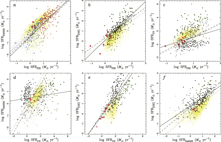
Figure 2. Comparisons of the four independently estimated SFRs from FIR luminosity, D4000, UV-luminosity, and [O ii]λ3727 luminosity for the AKARI-detected (small filled and open circles) and Herschel-detected objects (stars). In panel (a), blue and red symbols represent low-z ( ) and high-z (
 ) objects, respectively, and open symbols indicate red or old objects, i.e., D4000 > 1.8. In panels (c), (d), and (e), upper limits of the UV-based SFR are shown as open symbols. Gray symbols in panels (d) and (f) represent the red or old population, same as the open symbols in panel (a). Green-large circles mark highly obscured objects, i.e.,
  . The gray-dotted line indicates the one-to-one relation, and black solid and dashed lines are fitting results, i.e.,
  and
and  , respectively. Gray solid and dashed lines in panel (a) are best-fit for data excluding red or old objects. Yellow circles represent normal star-forming galaxies detected with AKARI.
Download figure:
Standard image High-resolution imageTable 1. Results of Correlation Fittings and the Spearman Rank-order Test

|

|
Spearman | Sample | Figure | ||||||||||
|---|---|---|---|---|---|---|---|---|---|---|---|---|---|---|
| x | y | a | b | rms | c | rms | ρ | p | ||||||

|

|
1.085 ± 0.041 | −0.464 ± 0.039 | 0.569 | −0.403 ± 0.026 | 0.571 | +0.79 |

|
⋯ | 2(a) | ||||
![${\mathrm{SFR}}_{[{\rm{O}}\;{\rm{II}}]}$](https://content.cld.iop.org/journals/0004-637X/807/1/28/revision1/apj513849ieqn74.gif)
|

|
1.281 ± 0.054 | 0.075 ± 0.058 | 0.546 | 0.334 ± 0.030 | 0.565 | +0.80 |

|
⋯ | 2(b) | ||||

|

|
0.621 ± 0.137 | 0.454 ± 0.137 | 1.387 | 0.164 ± 0.089 | 1.406 | +0.28 |

|
⋯ | 2(c) | ||||

|

|
0.091 ± 0.035 | 0.443 ± 0.059 | 0.786 | −0.403 ± 0.097 | 1.527 | +0.18 |

|
⋯ | 2(d) | ||||
![${\mathrm{SFR}}_{[{\rm{O}}\;{\rm{II}}]}$](https://content.cld.iop.org/journals/0004-637X/807/1/28/revision1/apj513849ieqn83.gif)
|

|
0.924 ± 0.077 | −0.159 ± 0.189 | 0.989 | −0.014 ± 0.069 | 0.989 | +0.66 |

|
⋯ | 2(e) | ||||
![${\mathrm{SFR}}_{[{\rm{O}}\;{\rm{II}}]}$](https://content.cld.iop.org/journals/0004-637X/807/1/28/revision1/apj513849ieqn86.gif)
|

|
0.805 ± 0.045 | 0.772 ± 0.043 | 0.635 | 0.655 ± 0.034 | 0.650 | +0.73 |

|
⋯ | 2(f) | ||||
![${L}_{\mathrm{AGN},[{\rm{O}}\;{\rm{III}}]}$](https://content.cld.iop.org/journals/0004-637X/807/1/28/revision1/apj513849ieqn89.gif)
|

|
0.611 ± 0.022 | 16.820 ± 0.998 | 0.321 | ⋯ | ⋯ | +0.82 |

|
Seyfert 2s | 3(a) | ||||
![${L}_{\mathrm{AGN},[{\rm{O}}\;{\rm{III}}]}$](https://content.cld.iop.org/journals/0004-637X/807/1/28/revision1/apj513849ieqn92.gif)
|

|
0.464 ± 0.038 | 23.509 ± 1.650 | 0.470 | ⋯ | ⋯ | +0.61 |

|
LINER 2s | 3(a) | ||||
![${L}_{\mathrm{AGN},[{\rm{O}}\;{\rm{III}}]}$](https://content.cld.iop.org/journals/0004-637X/807/1/28/revision1/apj513849ieqn95.gif)
|

|
0.494 ± 0.017 | 22.099 ± 0.776 | 0.384 | ⋯ | ⋯ | +0.81 |

|
Total | 3(a) | ||||
![${L}_{\mathrm{AGN},[{\rm{O}}\;{\rm{III}}]\&[{\rm{O}}\;{\rm{I}}]}$](https://content.cld.iop.org/journals/0004-637X/807/1/28/revision1/apj513849ieqn98.gif)
|

|
0.644 ± 0.022 | 15.414 ± 0.961 | 0.302 | ⋯ | ⋯ | +0.85 |

|
Seyfert 2s | 3(b) | ||||
![${L}_{\mathrm{AGN},[{\rm{O}}\;{\rm{III}}]\&[{\rm{O}}\;{\rm{I}}]}$](https://content.cld.iop.org/journals/0004-637X/807/1/28/revision1/apj513849ieqn101.gif)
|

|
0.485 ± 0.037 | 22.457 ± 1.642 | 0.456 | ⋯ | ⋯ | +0.63 |

|
LINER 2s | 3(b) | ||||
![${L}_{\mathrm{AGN},[{\rm{O}}\;{\rm{III}}]\&[{\rm{O}}\;{\rm{I}}]}$](https://content.cld.iop.org/journals/0004-637X/807/1/28/revision1/apj513849ieqn104.gif)
|

|
0.576 ± 0.018 | 18.478 ± 0.807 | 0.357 | ⋯ | ⋯ | +0.84 |

|
Total | 3(b) | ||||

|

|
0.119 ± 0.113 | 38.843 ± 5.045 | 0.705 | ⋯ | ⋯ | +0.17 |

|
X-ray AGN 1s | 4 | ||||

|

|
0.597 ± 0.171 | 17.746 ± 7.498 | 0.679 | ⋯ | ⋯ | +0.54 |

|
X-ray AGN 2s | 4 | ||||

|

|
0.661 ± 0.189 | 14.982 ± 8.315 | 0.720 | ⋯ | ⋯ | +0.54 |

|
SDSS AGN 1s | 4 | ||||

|

|
0.331 ± 0.081 | 29.440 ± 3.576 | 0.723 | ⋯ | ⋯ | +0.79 |

|
Total | 4 | ||||
Download table as: ASCIITypeset image
Second, we compared FIR-based and [O ii]λ3727-based SFRs in Figure 2(b). SFRs are measured and calibrated based on Hα and [O ii]λ3727 lines, mainly for normal galaxies (e.g., Kennicutt 1983, 1992; Kennicutt et al. 1994; Madau et al. 1998; Hopkins et al. 2003; Kewley et al. 2004; Moustakas et al. 2006). Recently, to derive attenuation-corrected line luminosities of galaxies, some studies have combined optical and infrared observations (e.g., Kennicutt et al. 2009; Domínguez Sánchez et al. 2012, and references therein). Unfortunately, because of AGN contributions, it is difficult to adopt such corrections for our AGN sample. The best-fit relation between SFR and SFR
![${}_{[{\rm{O}}\;{\rm{II}}]}$](https://content.cld.iop.org/journals/0004-637X/807/1/28/revision1/apj513849ieqn120.gif) (black-solid line) is steeper than the one-to-one correspondence, plausibly due to the combination of the following effects: the AGN contribution to the [O ii]λ3727 line, leading to an overestimation of the SFR, particularly for high [O ii]λ3727 luminosity objects, and the stronger aperture effect of the SDSS spectroscopy for lower-z, i.e., lower [O ii]λ3727 luminosity objects. Furthermore, for highly reddened objects, [O ii]λ3727-based SFR may become too high if extinction is over-corrected. It would also be necessary to consider metallicity and ionization conditions for the [O ii]λ3727 line. On the other hand, the FIR luminosity is contributed by dust in cirrus clouds that are warmed by diffuse starlight, particularly at low SFR (i.e., below 10
(black-solid line) is steeper than the one-to-one correspondence, plausibly due to the combination of the following effects: the AGN contribution to the [O ii]λ3727 line, leading to an overestimation of the SFR, particularly for high [O ii]λ3727 luminosity objects, and the stronger aperture effect of the SDSS spectroscopy for lower-z, i.e., lower [O ii]λ3727 luminosity objects. Furthermore, for highly reddened objects, [O ii]λ3727-based SFR may become too high if extinction is over-corrected. It would also be necessary to consider metallicity and ionization conditions for the [O ii]λ3727 line. On the other hand, the FIR luminosity is contributed by dust in cirrus clouds that are warmed by diffuse starlight, particularly at low SFR (i.e., below 10  yr−1). This overestimates of SFR
 results in a steeper slope both for AGNs and normal star-forming galaxies.
Third, the UV-based and FIR-based SFRs are compared in Figure 2(c). Many objects are located below the one-to-one line, indicating that UV-based SFR is largely underestimated presumably due to the dust extinction. Note that since UV detection is not available for all AGNs, we include upper limits of UV-based SFR (open symbols) while most obscured galaxies are marked with green circles. The large scatter between UV-based and FIR-based SFRs (see Table 1), suggests that the UV-based SFs are highly uncertain at any luminosity range, due to extinction and the contamination from AGB stars.
Fourth, Figure 2(d) presents a comparison of the UV-based SFR with SFR , illustrating no significant correlation between them. On the other hand, Figure 2(e) shows a good correlation between the SFR
 and SFR
![${}_{[{\rm{O}}\;{\rm{II}}]}$](https://content.cld.iop.org/journals/0004-637X/807/1/28/revision1/apj513849ieqn125.gif) . However, both SFRs suffer an extinction effect though there is a correlation between them.
. However, both SFRs suffer an extinction effect though there is a correlation between them.
Fifth, Figure 2(f) compares SFR and SFR
![${}_{[{\rm{O}}\;{\rm{II}}]}$](https://content.cld.iop.org/journals/0004-637X/807/1/28/revision1/apj513849ieqn127.gif) , showing a correlation with a systematic shift toward high SFR
, showing a correlation with a systematic shift toward high SFR![${}_{[{\rm{O}}\;{\rm{II}}]}$](https://content.cld.iop.org/journals/0004-637X/807/1/28/revision1/apj513849ieqn128.gif) . The larger SFR
. The larger SFR![${}_{[{\rm{O}}\;{\rm{II}}]}$](https://content.cld.iop.org/journals/0004-637X/807/1/28/revision1/apj513849ieqn129.gif) than SFR
than SFR is mainly due to the AGN contribution to the [O ii]λ3727 line, while normal star-forming spirals show no excess of SFR
![${}_{[{\rm{O}}\;{\rm{II}}]}$](https://content.cld.iop.org/journals/0004-637X/807/1/28/revision1/apj513849ieqn131.gif) .
.
For quantitative analysis, we calculated the Spearman rank-order correlation coefficient ρ and their statistical significance p for all available data excluding upper limits. As presented in Table 1, we confirmed that the UV-based SFR seems to show weak or almost no correlation with other indicators. FIR-based SFR seems to present slightly stronger correlations with optical-based SFRs than the relation among other SFRs, suggesting that FIR-based SFR is a reasonable SF indicator.
By comparing four independently estimated SFRs, we conclude that the FIR luminosity is the most reasonable SF indicator for host galaxies of type-2 AGNs. Thus, we will use the FIR luminosity as an SFR indicator, and compare it with the AGN luminosity in the following sections.
3.2. A Relation between FIR and AGN Luminosities
To examine the  –
– relation, we need to estimate AGN luminosities. X-ray luminosity is the most reliable indicator of AGN bolometric luminosity. However, it is not available for large samples including low-luminosity AGNs. The [Ne v]λ3426 line is also a good indicator to estimate AGN luminosities without a contamination from H ii regions (e.g., Gilli et al. 2010). Unfortunately, this emission line is typically weak and not covered by the SDSS wavelength range for objects at
  . As a number of previous studies of type-2 AGNs used the [O iii]λ5007 line luminosity as a proxy for AGN luminosities (e.g., Heckman et al. 2004; Kewley et al. 2006; Netzer et al. 2006; Kauffmann & Heckman 2009; Netzer 2009; LaMassa et al. 2013), we calculate bolometric luminosity from the [O iii]λ5007 line, adopting a bolometric correction, BC = 600 (e.g., Kauffmann & Heckman 2009; Netzer 2009). Figure 3(a) shows the relation between the FIR luminosity and AGN luminosity based on the [O iii]λ5007 line.

Figure 3. Relations between FIR luminosity at 90 or 100 μm, and AGN luminosity estimated from the [O iii]λ5007 line (the left-hand panel (a)) and the combination of the [O iii]λ5007 and [O i]λ6300 lines (the right-hand panel (b)). The AKARI-detected and Herschel-detected objects are denoted with small circles and stars, respectively. Vertical and horizontal bars show 1σ errors in their luminosities. Red and blue symbols indicate Seyfert 2s and LINER 2s, respectively. Blue-, red-, and purple-dashed lines are respective fitting results of Seyfert 2s, LINER 2s, and total objects. The reference line from Netzer (2009) is represented by black lines, assuming three different flux ratios (i.e.,  ), namely mean (the solid line), minimum and maximum ratios (dotted lines) from Dale & Helou (2002). The pure-AGN sequence with the 1σ range is calculated from an intrinsic-AGN SED, shown as gray lines. Six pure-AGN candidates are denoted with large-black circles in the panel (b). Light-green circles indicate composite objects selected with the BPT diagram, which are detected with AKARI.
Download figure:
Standard image High-resolution imageOn the other hand, Netzer (2009) claimed that using the [O iii]λ5007 luminosity as a proxy for the AGN bolometric luminosity is unreliable due to its dependence on the ionization parameter, which is critical for low-ionization sources such as LINERs. Thus, in order to avoid this ionization effect, we also calculated AGN bolometric luminosity from the combination of [O iii]λ5007 and [O i]λ6300 line fluxes, using the calibration given by Netzer (2009):

where ![${L}_{[{\rm{O}}\;{\rm{III}}]}$](https://content.cld.iop.org/journals/0004-637X/807/1/28/revision1/apj513849ieqn136.gif) and
and ![${L}_{[{\rm{O}}\;{\rm{I}}]}$](https://content.cld.iop.org/journals/0004-637X/807/1/28/revision1/apj513849ieqn137.gif) are extinction-corrected luminosities of [O iii]λ5007 and [O i]λ6300 lines, respectively, in units of erg s−1, using the Balmer decrement. Although the [O i]λ6300 line is much weaker than [O iii]λ5007, we determined reliable AGN bolometric luminosities for 492 objects with
are extinction-corrected luminosities of [O iii]λ5007 and [O i]λ6300 lines, respectively, in units of erg s−1, using the Balmer decrement. Although the [O i]λ6300 line is much weaker than [O iii]λ5007, we determined reliable AGN bolometric luminosities for 492 objects with  for the [O i]λ6300 line. Note that even in the extreme case, e.g.,
 ![${\rm{S}}/{{\rm{N}}}_{[{\rm{O}}\mathrm{III}]}=6$](https://content.cld.iop.org/journals/0004-637X/807/1/28/revision1/apj513849ieqn139.gif) and
and ![${\rm{S}}/{{\rm{N}}}_{[{\rm{O}}{\rm{I}}]}=3$](https://content.cld.iop.org/journals/0004-637X/807/1/28/revision1/apj513849ieqn140.gif) , the uncertainty of logarithmic AGN luminosity,
, the uncertainty of logarithmic AGN luminosity,  , is 0.25, and this is acceptable in our discussion. The relation between the FIR luminosity and AGN luminosity estimated by using the combination of two oxygen lines in Figure 3(b).
By comparing Figures 3(a) and (b), we examine which AGN luminosity estimate is more reliable in this study. To investigate the ionization parameter effect, we plotted Seyfert 2s and LINER 2s with different symbols (i.e., red and blue symbols, respectively). We confirmed that the relation with the [O iii]λ5007-based AGN luminosity shows a larger scatter than that with AGN luminosity based on the combination of the [O iii]λ5007 and [O i]λ6300 lines, particularly for LINER 2s at the low  range. We performed a liner fit to Seyfert 2s, LINER 2s, and total objects, finding that the [O iii]λ5007 and [O i]λ6300 combined method seems to correct for systematic trend in the distribution due to the ionization condition. By applying the Spearman rank-order test (see Table 1), we find a stronger correlation of FIR luminosity with AGN luminosity based on [O iii]λ5007 and [O i]λ6300 method than based on the [O iii]λ5007 only. These results imply that the ionization mechanisms of Seyfert 2s and LINER 2s are similar. Thus, in the following analysis, we use both Seyfert 2s and LINER 2s and adopt the AGN bolometric luminosity estimated by [O iii]λ5007 and [O i]λ6300 lines.
As shown in Figure 3, AKARI-detected objects show a clear trend between FIR and AGN luminosities, confirming the AGN-SF relation reported by previous studies. To directly compare with the previous studies, we included the reference line from Netzer (2009), which represents the relation between the D4000-based SF luminosity and AGN luminosity. Note that the reference line was revised by converting 60 μm luminosity to 90 μm luminosity using three different flux ratios, i.e.,  , −0.32, and 0.21, which are based on the different SED templates (Dale & Helou 2002). Our result is consistent with that of Netzer (2009) within the uncertainties of the FIR luminosity conversion. In contrast, we do not find strong evidence of the enhanced SF for given AGN luminosity, as reported by Rosario et al. (2012) for low-luminosity AGNs, particularly at high redshift, suggesting that low-luminosity AGNs are hosted by low-SF galaxies in the present day.
In addition, we plotted Herschel-detected objects as red stars. Since the flux limit of these objects are two orders of magnitude deeper than the AKARI/FIS survey, the additional Herschel sample helps us to overcome the flux limit of the shallow AKARI/FIS survey (see Figure 1). Herschel-detected objects are slightly shifted to a lower  ratio compared to AKARI-detected objects. Note that, as we described in Section 2, all type-2 AGNs in the COSMOS field are undetected with AKARI while most of them are detected with Herschel. On the other hand, ∼30,000 objects in the SDSS field are not detected with AKARI, implying that a large number of AGNs that are not detected with AKARI may occupy the region where Herschel-detected objects are located in Figure 3.
4. DISCUSSION
4.1. Type-1 AGNs versus Type-2 AGNs
We investigated the relation between FIR and AGN luminosities using type-2 AGNs, for which AGN bolometric luminosity is somewhat uncertain compared to type-1 AGNs. To overcome the uncertainty of the bolometric luminosity and to test whether type-1 AGNs also follow the same relation between FIR and AGN luminosities, we used X-ray AGN samples in this section.
First, we collected X-ray detected type-2 AGNs at  from Lusso et al. (2011), and matched them against the PEP catalog, finding six Herschel-detected sources. For these sources, we adopted AGN bolometric luminosities estimated using infrared and X-ray luminosities (Lusso et al. 2011). Second, we collected X-ray detected type-1 AGNs at the same redshift range from the COSMOS (Brusa et al. 2010). By matching them against the PEP catalog, we obtained three Herschel-detected X-ray AGNs. Third, we collected X-ray detected AGNs from the 70 months Swift-BAT all-sky hard X-ray survey catalog (Stern & Laor 2013). By matching them against the AKARI/FIS catalog, we obtained two X-ray detected type-1 AGNs and four X-ray detected type-2 AGNs. For these AGNs, we estimated the AGN bolometric luminosity from the X-ray luminosity with a bolometric correction in Rigby et al. (2009). Fourth, we collected 23 Seyfert 1s and 18 Seyfert 2s from the 12 micron galaxy sample (Spinoglio & Malkan 1989; Rush et al. 1993), which are detected in X-ray with XMM-Newton (Brightman & Nandra 2011). Using these four samples, we plotted 28 type-1 AGNs (blue) and 28 type-2 AGNs (red) detected in X-rays on Figure 4. These X-ray AGNs seem to generally follow a similar trend between FIR and AGN luminosities, albeit the small sample size. To quantitatively assess these trends, we plotted the best-fit linear relations, respectively, for X-ray type-2 AGNs and X-ray type-1 AGNs, and calculated the Spearman rank-order correlation coefficients (see Table 1). We find that X-ray type-2 AGNs show a similar relation to our SDSS type-2 AGNs, while X-ray type-1 AGNs seems to have a different slope. The shallow slope of X-ray type-1 AGNs seems to be due to the narrow
  range. A larger sample is required to examine the origin of the difference in slope. Note that systematic errors from different data sets, especially in estimations of AGN luminosities, would affect these comparisons.

Figure 4. Relation between FIR and AGN luminosities of type-1 and type-2 AGNs at  . The gray circles, stars, and lines are the same as in Figure 3(b). The X-ray type-2 and type-1 AGNs are represented by red and blue symbols, respectively. For each survey, individual symbols are given as labeled at the top left. In addition, SDSS type-1 AGNs with AKARI detections are also shown as yellow circles. Respective fitting results are shown as dashed lines with the same colors of each symbol.
Download figure:
Standard image High-resolution imageIn addition to X-ray AGNs, we selected optically selected type-1 AGNs using the SDSS low-luminosity AGN sample in Stern & Laor (2013), for which the broad Hα line is detected, enabling us to estimate AGN luminosity based on the Hα line luminosity based on a recipe in Greene & Ho (2005). By matching them against the AKARI/FIS catalog, we obtained 45 type-1 AGNs. For these objects, an AGN bolometric luminosity is estimated from the broad Hα line luminosity. In Figure 4, we plotted optical type-1 AGNs along with type-2 AGNs with yellow circles, showing that optical type-1 AGNs follow a consistent relation between FIR and AGN luminosities. We conclude the method of AGN bolometric luminosity estimation, i.e., narrow emission line luminosity, X-ray luminosity, and broad Hα luminosity, does not significantly affect the relation between FIR and AGN luminosities, and that optical type-1 and type-2 AGNs show a similar relation between FIR and AGN luminosities.
4.2. Comparisons with Previous Studies
In this section we compare our result with that of the previous studies. As shown in Figure 3, we found a similar relation between SF and AGN luminosities as reported by Netzer (2009). The difference between our study and that of Netzer (2009) is that while we used FIR luminosity as a proxy for SF, Netzer (2009) used D4000 in estimating SF luminosity. As discussed in Section 3.1, D4000-based SFR is not well determined at lower SFR since the calibration was based on starburst galaxies. Even with the FIR luminosity, which is a relatively better SF indicator, we find a similar relation between SF luminosity and AGN luminosity. This is probably due to the fact that the relation is not tight and the ratio between SF luminosity and AGN luminosity has a broad distribution, hence, the systematic difference between D4000-based SF luminosity and FIR luminosity is not clearly detected.
It is interesting to note that Herschel-detected objects follow a similar relation as AKARI-detected sources, i.e., low- AGNs at higher redshift, show the similar trend between FIR and AGN luminosities, suggesting that the relation is not due to the selection effect. In Figure 5, the luminosity limits with increasing redshift is demonstrated in the
  –
– plane. Here, we divided our sample into three redshift bins, i.e.,
  ,
,  , and
, and  , and the AKARI/FIS 5σ-detection limits at z = 0.01, 0.04, and 0.10 are denoted with dashed horizontal lines. As shown in Figure 5, the AKARI-detected sources are strongly affected by the Malmquist bias, indicating that the AKARI/FIS sample alone does not allow us to investigate the relation between FIR and AGN luminosities without suffering the selection effect due to the flux limit. In contrast, Herschel-detected sources enable us to examine the relation over a wide luminosity range at given redshift (e.g.,
  or
or  ). In particular, for AGNs at
  , the relation between FIR and AGN luminosities is detected over a wide range of AGN accretion luminosity,
  (erg s−1)
  . We conclude that the relation between FIR and AGN luminosities is not due to the flux limit of the AKARI/FIS surveys.

Figure 5. Redshift distributions of our type-2 AGNs on the  –
– plane. The sample is divided in three redshift bins,
  ,
,  , and
, and  , respectively, denoted with black, blue, and red symbols. The AKARI-detected and Herschel-detected objects are shown as open circles and filled stars, respectively. The luminosity limits at
  0.01, 0.04, and 0.10 based on the AKARI 5σ-detection limits are denoted with horizontal dashed lines. Gray lines are the same as those in Figure 3.
Download figure:
Standard image High-resolution imageTo investigate the effect of the flux limit for given redshift bins, we calculated the mean FIR luminosities of the AKARI-detected sources in each redshift bin, i.e.,  ,
,  , and
, and  , after dividing the AGNs in each redshift bin into subgroups based on AGN luminosity. In Figure 6, we present the mean FIR luminosities for each bin. The mean FIR and AGN luminosities show rather a flattened pattern in each redshift bin, compared to the relation between FIR and AGN luminosities of individual objects. In particular, at low AGN luminosity, the mean SF luminosity appears to be enhanced for fixed AGN luminosity, as similarly reported by recent studies (e.g., Shao et al. 2010; Rosario et al. 2012). However, this flattened pattern is not detected when we use individual luminosity measurements instead of mean luminosities (see also Netzer 2009). The reason why we do not find AGNs hosted by galaxies with enhanced SF (i.e., above the one-to-one relation in Figure 3) may result from our sample selection since we excluded the composite objects in the BPT selection. It is possible that we missed SF-enhanced AGNs, which could be classified as composite objects, i.e., star-burst AGNs. To check whether composite objects are distributed above our relation or not, we plot galaxies classified as composite objects based on the BPT method (shown as light-green circles in Figure 3). Note that AGN bolometric luminosities might be overestimated for composite objects because of the contamination from star formation. As shown in Figure 4, we investigated the
  –
– relation of X-ray selected objects and confirmed that several X-ray detected AGNs are distributed on the enhanced-SF area (top-left region in this figure), although its fraction is quite low, indicating that our results are consistent with Netzer (2009). A direct test with the SDSS composite objects is difficult to perform since the AGN luminosity estimated from the narrow emission lines would be much more uncertain due to the contribution from SF. Note that Rosario et al. (2012) adopted 60 μm luminosity as an SF indicator which may be more contaminated by an AGN component than 90 and 100 μm luminosities (e.g., Spinoglio et al. 2002), and their mean FIR luminosities may be overestimated. Moreover, if Rosario et al. (2012) lost low X-ray luminosity objects, which would show low FIR luminosities in their sample selection, their averaged FIR luminosities would be overestimated though they calculated mean FIR luminosities by considering FIR detected and undetected objects.

Figure 6. Mean FIR luminosities of the AKARI-detected objects for each  bin. The mean luminosities in each redshift range,
  ,
,  , and
, and  , are denoted with black, blue, and red circles, respectively. For each mean value, vertical bars represent 3σ errors while horizontal bars show the AGN-luminosity ranges. If the sample size is less than two in a bin, a filled circle without error bars is given. The Herschel-detected objects are shown as filled stars. Horizontal and gray lines are the same as in Figure 5.
Download figure:
Standard image High-resolution image4.3. AGN Contribution to FIR Luminosities
If there are luminous AGNs hosted by low-SF galaxies, we may find them at the bottom right of the  –
– plane (see Figure 3). Usually, the AGN contribution to FIR is believed to be negligible, since SF galaxies dominate at FIR. When very low FIR luminosities are probed, however, it is necessary to quantify the AGN contribution. To investigate the FIR luminosities of a pure-AGN without SF, we adopted an SED template from Mullaney et al. (2011). Using the strong correlation between the MIR (12.3 μm) and the X-ray (2−10 keV) luminosities from Gandhi et al. (2009), we obtained the MIR luminosity as a function of AGN luminosity (see also Ichikawa et al. 2012), then calculate the FIR luminosity based on the pure-AGN SED template. In this process, we estimated the AGN bolometric luminosity from the X-ray luminosity (Rosario et al. 2012).
In Figure 3, the estimated pure-AGN sequence is denoted with gray lines. Based on a comparison of our sample with the pure-AGN sequence, we found that the AGN contribution in our sample seems to be negligible, although there are six objects reaching this pure-AGN sequence. Note that it is important to examine these objects located on the pure-AGN sequence since they are likely to be low-SF AGNs compared to the star-forming galaxies in our sample, if the expectation of contribution to FIR luminosities from the intrinsic-AGN SED is correct (see also Mor & Netzer 2012; Rosario et al. 2012).
4.4. Spectral Energy Distributions
For understanding the  –
– relation in detail, in this section we investigate SEDs of our type-2 AGNs. As we mentioned in Section 4.3, six objects are located close to the pure-AGN sequence. Here, we focus on these objects as pure-AGN candidates, i.e., luminous AGNs hosted by no- or low-SF galaxies (see large circles in Figure 3). Using multi-wavelength data, i.e., SDSS-optical, AKARI-FIR, WISE-MIR, and GALEX-UV data, we separately constructed the composite SEDs of pure-AGN candidates and AGNs hosted by star-forming galaxies shown in Figure 7. First, we normalized all-band luminosities with the SDSS R-band luminosity. Note that this normalization is effectively a stellar mass normalization, since optical-NIR luminosities roughly represent the stellar mass. In this construction, we used 5σ upper limits for undetected sources. Along with the SEDs, we plotted three SED templates: a starburst galaxy IRAS 19254−7245, NGC 6240 (starburst + Seyfert 2), and a composite SED of Seyfert 2 galaxies (Polletta et al. 2007) as gray lines in Figure 7. These template SEDs are also normalized at the SDSS R-band wavelength.

Figure 7. Composite SEDs of pure-AGN candidates (red) and star-forming AGNs (black), normalized with SDSS R-band luminosity. Three representative SEDs are also shown as gray lines: starburst galaxy IRAS 19254−7245 (solid line), NGC 6240 (dashed line), and an average Seyfert 2 galaxy (dash–dot line).
Download figure:
Standard image High-resolution imageAs shown in Figure 7, we confirmed that the FIR luminosities of pure-AGN candidates are lower than AGNs hosted by star-forming galaxies, as already suggested in Figure 3. This indicates that pure-AGN candidates have significantly lower-SF host galaxies relative to star-forming AGNs. As SF indicators, UV luminosities also show a similar trend to the FIR luminosities, i.e., UV luminosities of pure-AGN candidates are lower than star-forming AGNs, although UV luminosities suffer from uncertainties as described in Section 3.1. Moreover, in the optical range, there is a difference of spectral slope between pure-AGN candidates and star-forming AGNs, suggesting the difference of D4000 between two groups. On the other hand, MIR luminosities, which are indicators of the AGN luminosity, show no significant difference between pure-AGN candidates and star-forming AGNs. These results indicate that for given stellar mass, the AGN luminosity is comparable between pure-AGN candidates and star-forming AGNs while pure-AGN candidates have on average lower SF than star-forming AGNs. Compared to the templates, we found that the SED of pure-AGN candidates is located between NGC 6240, which is a composite of starburst and Seyfert 2, and Seyfert 2 templates while the SED of star-forming AGNs is similar to the template of NGC 6240. This indicates that pure-AGN candidates are hosted by significantly lower-SF galaxies than star-forming AGNs. Note that even pure-AGN candidates have higher FIR luminosities than the Seyfert 2 template, probably due to the AKARI flux-limit. In other words, AKARI sample is biased toward active star-forming hosts.
To understand the dependency of the SEDs in relation with  and
and  , we divided our sample into subsamples by using FIR luminosities or accretion luminosities: we adopted AGN-luminosity bins of
  ,
,  , and
, and  , and for FIR-luminosity bins we used
  ,
,  , and
, and  . For each bin, we constructed an average SED as plotted in Figure 8.

Figure 8. Composite SEDs of pure-AGN candidates and star-forming AGNs, for three AGN-luminosity bins (left-hand panels), and for three FIR-luminosity bins (right-hand panels). The lines are the same as in Figure 7.
Download figure:
Standard image High-resolution imageIn the left hand panels, the SEDs for three  bins are shown from bottom to top with increasing accretion luminosities. In the case of star-forming AGNs shown as black lines, FIR and UV luminosities are increasing with increasing AGN luminosities. as expected from the positive trend between FIR and AGN luminosities. Also, we found that more luminous objects show slightly flatter slopes in the optical range, again suggesting the correlation between SF and AGN luminosities at fixed stellar mass. Moreover, we confirmed that the WISE continuum seems to increase with AGN luminosities, indicating that MIR bands would also be good
  indicators (e.g., Gandhi et al. 2009). For each AGN luminosity bin (top and middle panels) the SEDs of pure-AGN candidates show lower-SF activities than star-forming AGNs, which is consistent with the result in Figure 7.
When we divided the sample into three  bins as plotted in the right hand panels, we found that FIR and UV luminosities (i.e., SF indicators), and MIR luminosities (i.e., a tracer of AGN accretion) are increasing together as expected from the positive
  –
– trend. The spectral slopes in the optical range are increasing with increasing FIR luminosities, reflecting the decrease of the D4000 (increase of SF). Note that the spectral slopes in the MIR range become steeper with increasing FIR luminosities, implying that there is an SF contribution to MIR luminosities. In the case of pure-AGN candidates (middle and bottom panels), pure-AGN candidates show higher MIR luminosities than star-forming AGNs, as expected from the trend in Figure 3 that pure-AGN candidates have higher AGN luminosities than star-forming AGNs at fixed FIR luminosities.
Based on the SED analysis with FIR and AGN luminosity bins, we confirmed that pure-AGN candidates are hosted by low-SF galaxies compared to star-forming AGNs. Thus, these pure-AGN candidates could be a crucial sample for understanding the AGN–SF connection. Since the fraction of such objects appears to be small,  , this population may not be dominant in black hole growth history. However, it is possible that we are missing low-SF AGNs on the
  –
– plane due to the observational limitations (see Section 4.5).
4.5. The Effects of the Flux Limit and Volume Limit
To better understand the observed relation between FIR and AGN luminosities in Figure 3, in this section we investigate the effects of the flux and volume limits by simulating the number density in the  –
– plane. Observationally it is difficult to find objects with high
  and low
  due to the following two effects:
- 1.at lower redshift, e.g.,
 , it is difficult to detect high- AGNs due to the limited survey volume,
 - 2.at higher redshift, e.g.,, objects with high are easier to detect, however, the flux limits of the FIR survey prevent the detection of low- galaxies hosting high- AGNs.


To quantify these effects, we simulate the distribution of AGNs as a function of AGN luminosity using the [O iii]λ5007 luminosity function derived from the COSMOS and SDSS type-2 AGN samples (Bongiorno et al. 2010). First, we calculated survey volumes for each redshift bin using the survey areas of the SDSS DR7 (i.e., 9380 deg2) and the PEP-COSMOS field (i.e., 2.0069 deg2), respectively, for the AKARI and Herschel samples. Then, using the flux limits, i.e., 0.55 Jy for the AKARI/FIS survey and 7.5 mJy for the Herschel/PACS survey, we estimated object numbers for each area box with a fixed size ( and
and  ), with increasing redshift. Finally, we integrated the number of objects over the redshift range
  .
.
Figure 9 presents the simulation results for the AKARI survey and the Herschel survey along with the observations. For simplicity, we adopted a [O iii]λ5007 line as a proxy for the AGN bolometric luminosity with a bolometric correction, BC = 600 (e.g., Kauffmann & Heckman 2009; Netzer 2009), since we used the [O iii]λ5007 luminosity function. The simulated distribution well reproduces the observed  –
– relation. Note that since we did not include the FIR luminosity function in our simulations, the top-left area shows very high object numbers. However, if we apply an FIR luminosity function, the object number in this area would decrease to zero.

Figure 9. Simulations of the  –
– distribution, demonstrating the effect of the flux limits in the AKARI/FIS all sky survey (left-hand panel), and the limited volume of the Herschel/PACS survey (right-hand panel). The logarithmic number density is calculated for each area bin with a size
  and
and  , and represented with different colors. For comparison, the AKARI-detected and Herschel-detected sources are also plotted with gray circles and red stars, respectively, while the pure-AGN sequence is denoted with white lines.
Download figure:
Standard image High-resolution imageOur simulation clearly indicates that the flux limit of the AKARI/FIS survey is insufficient to explore AGNs hosted by low-SF galaxies, close to the pure-AGN sequence while the limited volume of the PEP-COSMOS survey prevents us from detecting high  and low
  sources. We conclude that the combination of the AKARI-detected and Herschel-detected AGNs used for our investigation suffers the observational limitations due to the flux limit and the survey volume. Thus, we were not able to investigate the number density of the pure AGNs or AGNs in post-starburst galaxies with the AKARI/FIS and Herschel/PACS data. For a better understanding of the
  –
– relation, it is necessary to have wide and deep FIR surveys with the next-generation infrared astronomy missions, e.g., the Space Infrared Telescope and Cosmology and Astrophysics (SPICA).
5. SUMMARY AND CONCLUSIONS
To understand the AGN-SF connection, we investigated the relation between AGN and SF luminosities for a sample of SDSS type-2 AGNs at  , based on the AKARI/FIS all-sky survey and the PEP COSMOS survey. We estimated AGN luminosities from [O iii]λ5007 and [O i]λ6300 emission lines, and utilized the proposed linear proportionality of SFR with FIR luminosities in Kennicutt's equation. The main results are summarized as follows.
- 1.By comparing four independent SF indicators, i.e., FIR-based, UV-based, D4000-based, and [O ii]λ3727-based SFRs, we find that the FIR luminosity is the most acceptible and less subjective to AGN contamination compared to other SF indicators (Section 3.1).
- 2.
- 3.Using X-ray AGNs and optical type-1 AGNs, we find a similar relation between and , suggesting that the observed relation is not significantly affected by the method and uncertainty of the AGN bolometric luminosity estimation (Section 4.1).
- 4.The flux limit of AKARI FIR survey significantly affects the distribution in the– plane while deep-FIR data such as in the Herschel survey can overcome the limitation. It is possible that the AKARI FIR-detection limit is responsible for the observed trend in the and plane (Section 4.2).
- 5.FIR luminosities of most type-2 AGNs are dominated by the non-AGN continuum, while the AGN contribution to FIR emission is negligible (Section 4.3).
- 6.Based on the simulation of the AGN number distribution, we showed that the observed– relation can be explained by the flux limit of the AKARI/FIS survey and the limited volume of the Herschel/PACS survey, demonstrating the limitations of the current survey data for detecting and investigating luminous AGNs hosted by low-SF galaxies (Section 4.5).


Although it is possible that the observational limitations may cause an artificial correlation between FIR and AGN luminosities, the observed positive relation may suggest an intrinsic connection between SF and AGN activities in the present-day, implying that the growth of stellar mass and black hole mass are linked at least in the AGN phase in galaxy evolution. Quantifying the number density of luminous AGNs in low-SF or non-SF galaxies requires wide and deep future FIR surveys, e.g., SPICA.
We would like to thank Tohru Nagao and Hagai Netzer for their helpful comments and suggestions, and thank Hyun-Jin Bae for the contribution of the line flux measurements. We also thank Matthew A. Malkan for his useful comments and suggestions which improved the clarity our paper. We also thank David Rosario for his useful comments. This work has been supported by the National Research Foundation of Korea (NRF) grant funded by the Korea government (No. 2012-006087 and No. 2013-K2A1A2055130). K.M. acknowledges financial support from the Japan Society for the Promotion of Science (JSPS). Data analyses were in part carried out on the common-use data analysis computer system at the Astronomy Data Center, ADC, of the National Astronomical Observatory of Japan (NAOJ). Funding for the SDSS and SDSS-II has been provided by the Alfred P. Sloan Foundation, the Participating Institutions, the National Science Foundation, the U.S. Department of Energy, the National Aeronautics and Space Administration, the Japanese Monbukagakusho, the Max Planck Society, and the Higher Education Funding Council for England. The SDSS Web Site is http://www.sdss.org/. The SDSS is managed by the Astrophysical Research Consortium for the Participating Institutions. The Participating Institutions are the American Museum of Natural History, Astrophysical Institute Potsdam, University of Basel, University of Cambridge, Case Western Reserve University, University of Chicago, Drexel University, Fermilab, the Institute for Advanced Study, the Japan Participation Group, Johns Hopkins University, the Joint Institute for Nuclear Astrophysics, the Kavli Institute for Particle Astrophysics and Cosmology, the Korean Scientist Group, the Chinese Academy of Sciences (LAMOST), Los Alamos National Laboratory, the Max-Planck-Institute for Astronomy (MPIA), the Max-Planck-Institute for Astrophysics (MPA), New Mexico State University, Ohio State University, University of Pittsburgh, University of Portsmouth, Princeton University, the United States Naval Observatory, and the University of Washington. This research is based on observations with AKARI, a JAXA project with the participation of ESA. Herschel is an ESA space observatory with science instruments provided by European-led Principal Investigator consortia and with important participation from NASA.
Footnotes
- 3
- 4
- 5