


ABSTRACT
We report analysis of three solar flares that occur within 1° of limb passage, with the goal to investigate the source height of chromospheric footpoints in white light (WL) and hard X-rays (HXR). We find the WL and HXR (≥30 keV) centroids to be largely co-spatial and from similar heights for all events, with altitudes around 800 km above the photosphere or 300–450 km above the limb height. Because of the extreme limb location of the events we study, emissions from such low altitudes are influenced by the opacity of the atmosphere and projection effects. STEREO images reveal that for SOL2012-11-20T12:36 the projection effects are smallest, giving upper limits of the absolute source height above the nominal photosphere for both wavelengths of ∼1000 km. To be compatible with the standard thick target model, these rather low altitudes require very low ambient densities within the flare footpoints, in particular if the HXR-producing electrons are only weakly beamed. That the WL and HXR emissions are co-spatial suggests that the observed WL emission mechanism is directly linked to the energy deposition by flare accelerated electrons. If the WL emission is from low-temperature ( K) plasma as currently thought, the energy deposition by HXR-producing electrons above ∼30 keV seems only to heat chromospheric plasma to such low temperatures. This implies that the energy in flare-accelerated electrons above ∼30 keV is not responsible for chromospheric evaporation of hot (
 K) plasma, but that their energy is lost through radiation in the optical range.
Export citation and abstract BibTeX RIS
1. INTRODUCTION
White light (WL) and hard X-ray (HXR) observations provide the most direct means of investigating the energy release and particle acceleration during solar flares. The WL/UV continuum in particular dominates the flare energy emitted in the electromagnetic spectrum. HXR emissions are produced by flare-accelerated electrons through the bremsstrahlung mechanism, most prominently in the chromospheric footpoints of flare loops where the electrons lose their energy through collisions with the ambient plasma (for reviews see Fletcher et al. 2011; Holman et al. 2011; Kontar et al. 2011). HXR footpoints are generally only seen from some parts of the flare ribbon structure, indicating that efficient electron acceleration is only associated with some particular loops within the flare arcade. The WL emissions in solar flares also originate from the flare ribbons via a thermal mechanism that is presently not well understood.
The WL and HXR emissions are closely correlated in time (e.g., Rust & Hegwer 1975; Hudson et al. 1992; Fletcher et al. 2007), intensity (e.g., Neidig & Kane 1993; Sylwester & Sylwester 2000; Chen & Ding 2005; Wang 2009; Watanabe et al. 2010), and in space (e.g., Xu et al. 2004, 2006; Krucker et al. 2011). This strongly suggests that the energy deposition by flare-accelerated electrons is intimately linked to the radiative output seen in WL. Temporal correlation shows a near-simultaneous onset of both emissions, with a longer decay time of the WL emission indicative of a cooling process. The close correlation in space suggests that the WL emission occurs in the same magnetic structures in which energetic electrons are depositing their energy. Quantitative comparison of the energy deposition and radiative output suffer from the lack of sufficiently complete spectral observations in the WL/UV range (e.g., Milligan et al. 2014). A blackbody spectrum is sometimes assumed, and it can be shown that the energy in flare-accelerated electrons assuming a thick target model is indeed large enough to account for the radiative losses in the optical range (e.g., Rieger et al. 1996; Watanabe et al. 2010; Kerr & Fletcher 2014).
Recent observations revealed very narrow ribbon structures, in particular with recent high resolution optical telescopes; generally the WL emission is patchy and unresolved, with ribbon structuress as narrow as 100 km (e.g., Xu et al. 2006; Sharykin & Kosovichev 2014). RHESSI observations also show that the HXR ribbons are narrow, with widths unresolved at below ∼800 km (Dennis & Pernak 2009; Krucker et al. 2011) The height of energy deposition in solar flare ribbons is difficult to observe because of small scale heights.
The altitude of the HXR source derived from the standard flare model, applying the thick-target approximation for electron propagation, relies on several assumptions. Its predictions are therefore ambiguous, even accepting the basic idea that the electron acceleration must occur in the corona (see e.g., Fletcher et al. 2011): (1) The altitude depends strongly on the assumed density model of the flaring atmosphere, with low-density models giving altitudes from as low as ∼600 km while high-density models can give altitudes up to several 1000 km (Battaglia & Kontar 2012, Figure 2). (2) There is a dependence on electron energy as deeper penetration is possible for electrons at higher energies, but this effect is is only a few hundreds of kilometers for energies above 30 keV (Battaglia & Kontar 2012, Figure 1). (3) There is weak dependence on the ionization level of the flaring atmosphere, with values differing by up to ∼200 km (Battaglia & Kontar 2012, Figure 3). (4) There is a significant dependence on the initial pitch-angle distribution of the accelerated electrons because of the effects of pitch-angle scattering and magnetic mirroring. (5) Field lines could be tilted relative to the radial direction giving higher altitudes for a given radial density distribution. The combined effects (excluding the tilt) give a difference of ∼500 km between strongly beamed and broadly beamed models (Battaglia & Kontar 2012, Figure 7). For the energy range relevant for this paper, around 30 keV (i.e., the range with the best counting statistics in the non-thermal range), the range of expected altitudes can be summarized as lying between ∼800 and ∼1500 km, if high-density models are excluded and field lines in the radial direction are assumed. The values at the lower end come from the more strongly beamed models, but these are unlikely as other observations have shown little evidence for strong beaming (e.g., Kontar et al. 2006). Hence, the values at the upper end of the theoretical range are perhaps favored for the standard thick target model, but even this is uncertain, as the density structure of a flaring footpoint is essentially unknown and is likely to differ from the standard density models assumed to derive these altitudes. Furthermore, for field lines different from radial directions (e.g., Smith et al. 2003) the thick target source locations would be expected at higher altitudes as well. Modified versions of the standard thick-target model involving local or global re-acceleration of electrons initially accelerated in the corona (e.g., Karlicky 1995; Turkmani et al. 2006; Brown et al. 2009; Gordovskyy & Browning 2012; Varady et al. 2014) can provide lower altitudes of the energy deposition, but do not address the re-acceleration in a quantitative way. If the energy transport from the coronal energy release region is done by waves instead of particles (Fletcher & Hudson 2008), the location of the HXR emission could potentially be lower than the predication from the thick target models, although acceleration at higher densities (lower altitudes) is generally excepted to be less effective as collisional loses increase with increasing density.
Conclusive observations of the absolute altitude of the HXR and WL source could be provided by direct observations of at least two widely different viewing angles. Currently there is no such combination of observatories available; Solar Orbiter might provide such an opportunity for both WL and HXR from a deep-space platform, but its requirements on absolute pointing knowledge for HXR are stringent and potentially difficult to match. The closest currently available set of observations comes from combined observations by the Helioseismic and Magnetic Imager (HMI)/RHESSI/STEREO (Martínez Oliveros et al. 2012), where the STEREO EUV ribbon locations are used as a proxy for the WL and HXR ribbon locations. This method only works for flares that are close to disk center as seen from STEREO and close to the limb (but on the front side) for RHESSI and SDO, in which case the uncertainties due to the use of UV as a proxy for the WL emission become small. The Martinez Oliveros results describe a single flare, giving altitudes for the WL and HXR footpoints of 305 ± 170 km and 195 km ± 70 km, respectively. These values are below the lowest of the expected values from the thick target model discussed above, indicating a fundamental flaw in the model or a radically different density distribution in the flaring atmosphere than that expected. A confirmation of these first results through further events is currently being eagerly awaited.
This paper combines solar flare observations from the HMI (Scherrer et al. 2012) and the RHESSI (Lin et al. 2002) where the WL and HXR emission are seen above the solar limb. The goal of this study is to set further observational constraints on the height structure of the WL and HXR emission of flare ribbons. Although the ribbon structure is seen from the side, the observed altitude does not necessarily give the absolute altitude for two reasons (see Figure 1 for a sketch of the possible geometries): (1) The effect of occultation might make the observed source height appear at a lower altitude. (2) Emission from below  generally cannot escape, which will tend to move the centroid to a higher altitude and make the source appear fainter. For the optical observations, the limb (typically defined as the inflection point of the image profile at 5000 Å) is expected to be around ∼350 km (Haberreiter et al. 2008) above
  , although Brown & Christensen-Dalsgaard (1998) place it nearer to 500 km. Allen (1973) identifies the limb at 5000 Å as
  , also defining the base of the chromosphere, and in the VAL-C model this opacity occurs at 370 km. The limb height in standard semi-empirical atmospheric models refers to optical depth, rather than a true spatial dimension, with a normalization at an accepted value of R
 . This height is not unique, because horizontal structure ("roughness," for example that associates with convection or p-modes) is known to be present, though difficult to characterize. Hence, low-altitude sources such as those reported by Martínez Oliveros et al. (2012) would not be visible when seen at the exact limb. Another influence on the absolute height of the WL emission may be due to the Wilson depression (e.g., Wilson & Cannon 1968), which lowers the height of emergence of visible light in sunspot umbrae by typically a few 100 km. The wide range of depression heights in the literature (up to 1000 km in the umbra) shows that this is a non-trivial problem in general (Solanki 2003 and references therein). For reference, the hard X-ray limb of the Sun due to Compton scattering is expected to be ∼450 km above R
 , not far from the optical limb (e.g., Martínez Oliveros et al. 2012). Despite all of these limitations, the imaging observations presented in this paper provide new insights into the radial structure in WL and HXR flare ribbons. In particular, the relative altitude of the HXR (location of energy deposition) to the WL (location of radiative losses), which is unaffected by these limitations, is of crucial importance for flare energetics.

Figure 1. Cartoon of potential scenarios for the interpretation of the observed altitudes of chromospheric sources near the limb. The black area represents the solar disk as seen from the polar region, out to its true radial distance  . The dashed line indicates the limb (inflection point), below which emission cannot freely escape. The red circles give the altitude of chromospheric source with the arrow pointing in the direction of escaping radiation toward an observatory near Earth. On the left, the ideal scenario with a source exactly in the plane of the sky and above the limb is shown. For the scenario where the source is slightly behind or in front of the limb as seen from Earth, the observed source gives a slightly lower altitude. The next two scenarios shown to the right highlight the fact that sources from low altitudes are invisible and that for elongated sources reaching below the inflection point only the top part can be seen. The scenario to the far right also includes fine structure such as the Wilson depression.
Download figure:
Standard image High-resolution image2. OBSERVATIONS
This study combines observations from three space-based observatories: HMI, RHESSI, and EUVI onboard STEREO.
HMI onboard the Solar Dynamic Observatory (SDO) is used to study WL emission at 617.3 nm at a spatial resolution of ∼1 1 FWHM (
 pixel size). Standard level 1.5 data products at a 45 s cadence are used. The Sun center is known to much better than 01 by direct limb fits, making use of the whole-Sun images, and by using the limb fits at position angles near the flare.
Since RHESSI records single photons, the exact time and duration of the HMI images can be matched (Smith et al. 2002). The RHESSI images shown are reconstructed using the standard RHESSI Clean algorithm with a reconstructed beam corresponding to RHESSI's maximal resolution of ∼2 3 (Hurford et al. 2002). The RHESSI requirement for absolute pointing to Sun center is better than 04 (Fivian et al. 2002). The inflight accuracy is significantly better than this, with values of the order of 015. In first order (i.e., for randomly distributed errors), this uncertainty blurs the RHESSI image, but does not change the source location. Only for higher orders (i.e., for the case that the errors are systematic) could the position be biased. The uncertainty on the RHESSI absolute pointing is therefore not considered significant relative to the errors from counting statistics that are typically of the order of 05 (∼100 km) for events with good counting statistics. The absolute source location accuracy of a combined HMI and RHESSI study is therefore generally high: Martínez Oliveros et al. 2012 have shown that combined uncertainties for their event was  (∼140 km). The largest systematic unknown in the error budget is the inflight separation of the RHESSI grids (i.e., the length of the tube that holds the grids) that is linearly proportional to the RHESSI height scale (distance from Sun center). Generally, the pre-flight value of the tube length (∼1.5 m) is used in the standard software. Laboratory measurements taken with the qualification model of the RHESSI tube showed that outgassing of the RHESSI carbon fiber tube makes the tube shrink asymptotically by ∼45 μm on a time scale of 23 days. The flight module of the RHESSI tube should have the same outgassing behavior as seen in the pre-flight test. It is therefore expected that the RHESSI resolution decreased by a fraction of 3 × 10⁻⁵ due to outgassing. At the limb, this has the effect of increasing the altitudes by ∼0 03 (∼22 km). Since this uncertainty is smaller than the statistical errors, the altitudes given in this work are not corrected for this effect. For completeness, a further, but even less significant systematic error due to the uncertainty of the calibration temperature of the RHESSI grids is mentioned here as well. The grid optical characterization was done at room temperature, without specifically controlling or recording the actual temperature resulting in an uncertainty in the temperature of the grids of a few degrees. The actual grid pitch relative to the nominal pitch is therefore unknown by a few times the thermal expansion coefficient. For the finest grid, the thermal expansion coefficient is 5 × 10⁻⁶ K−1 and the uncertainties become of the same order as for the probable outgassing effect for a ∼6 K temperature uncertainty. It is rather unlikely that the grid calibration was done that far away from room temperature. This second systematic error can increase or decrease the derived altitude, but overall, the uncertainties are not important compared to the statistical uncertainties. In summary, the RHESSI altitudes such as those given in this paper are dominated by the statistical uncertainties due to counting statistics with values of the order of 015 (∼100 km).
The different viewing angle provided by the EUVI instrument (Howard et al. 2008) onboard the STEREO mission (Kaiser et al. 2008) is used to determine the location and extent of the flare ribbons to estimate the effect of foreshortening and occultation of the ribbons as seen by HMI and RHESSI at the limb. The limb location as seen from Earth and the line-of-sight (LOS) through the WL and HXR has been calculated and over plotted on EUVI images of each flare, by using the standard information given in the relevant headers of the data files. A best estimate is derived by considering the brightest feature in each EUV ribbon to be the most likely counterpart of the WL and HXR sources, and for each event we additionally pick a conservative range of values for the maximal extent of the ribbon structures.
From the extensive database of flare events jointly observed by HMI and RHESSI (for other examples of such observations see Kosovichev 2011; Martínez Oliveros et al. 2011, 2012, 2014; Alvarado-Gómez et al. 2012; Saint-Hilaire et al. 2014), three events with WL and HXR emission seen clearly above the solar limb are presented in this paper. A systematic search of combined HMI and RHESSI limb flares is currently in preparation. For each flare with a location within  of the limb (an occultation by an angle
  gives a height
  km, close to the uncertainties of the absolute pointing), we should have ∼45 suitable on-disk flares. Hence, among the ∼80 M- and X-class flares that SDO typically observes per year (Aschwanden et al. 2014), we expect about ∼2 flares right at the limb. The RHESSI day-night cycle gives us a 60% chance of catching such flares, and so we predict around 5 events within the ∼4 y of combined SDO/RHESSI observations. Hence, there might be a few more events hidden in the database besides the three events discussed here, but likely not many. The selected events have GOES flare classes M7.7 (SOL2012-07-19T05:58), M1.7 (SOL2012-11-20T12:36), and X1.7 (SOL2013-05-13T12:36), respectively. Overview time profiles and images are given in Figures 2 and 3. In the following section, we describe the individual events, and follow with a discussion of the results as summarized in Table 1.
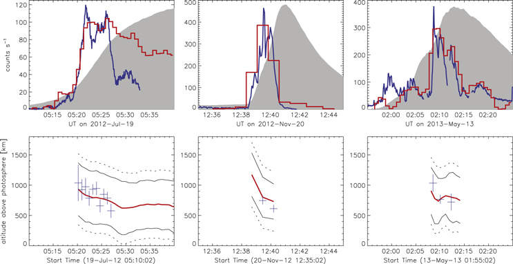
Figure 2. Time profiles of the three flares: the top panels show the time profiles of the WL flux (summed over enhancement; arbitrary units) and non-thermal HXR flux at 30–80 keV in red and blue, respectively, with the linear GOES curve shown schematically in gray in the background for timing reference. Below, the apparent altitude of the peak of the WL emission above the limb is shown in red. The black dotted lines give the FWHM of a Gaussian fit to the HMI source above the limb; the thin black line is the deconvolved source size derived by a rough deconvolution of the observed size with the HMI PSF from Yeo et al. (2014). The blue points give the HXR centroid positions with error bars from statistical uncertainties. No error bars are shown for the HMI centroids as they are dominated by systematic uncertainties (∼70 km).
Download figure:
Standard image High-resolution image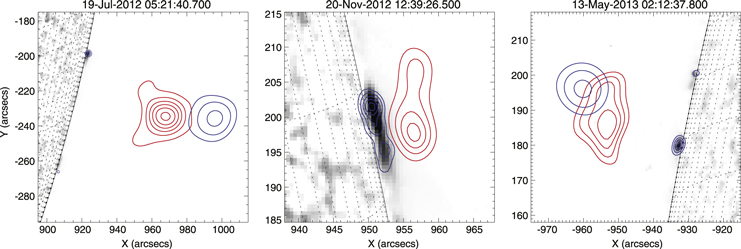
Figure 3. X-ray and optical imaging of the three flares at the peak time of the impulsive phase: the images are from HMI with the pre-flare image subtracted; enhanced emission is shown in black. The contours represent RHESSI Clean maps in the thermal (red, 12–15 keV) and non-thermal (blue, 30–80 keV) HXR range. Two flares (left and right) are large-scale flares with widely separated ribbons and flare loops reaching high altitudes, while the other flare (middle) is more compact. For all flares the ribbons appear above the limb. The large-scale flares show a non-thermal above-the-loop-top source.
Download figure:
Standard image High-resolution imageTable 1. Parameters of the WL (617.3 nm) and HXR (30–100 keV) Footpoints (Values of the Stronger Footpoint (see Figure 5) are Shown in Bold)
| Parameters | 2012 Jul 19 | 2012 Nov 20 | 2013 May 13 |
|---|---|---|---|
| HMI time | 05:21:40.7 | 12:39:26.5 | 02:12:37.8 |
| GOES flare class | M7.7 | M1.7 | X1.7 |
| Locationa of N ribbon (best guessb) | +0 7 7
|
−05
|
−10 |
| Projection effectb N (best guessb) | 51 km | 27 km | 105 km |
| Location of N ribbon (conservativeb) | +22 to −14
|
−01 to −13
|
+12 to −22 |
| Projection effect N (conservativeb) | <500 km | <180 km | <500 km |
| Location of S ribbon (best guessb) | −10 |

|
−12
|
| Projection effect S (best guessb) | 104 km | 39 km | 150 km |
| Location of S ribbon (conservativeb) | +05 to −18 |
−01 to −13 |
+24 to −41
|
| Projection effect S (conservativeb) | <340 km |
 km km |
<1800 km |
| WL altitude | 824 ± 70 km | 799 ± 70 km | 810 ± 70 km |
| WL radial extent (FWHM) | ∼862 km | ∼652 km | ∼839 km |
| HXR altitude | 946 ± 103 km | 746 ± 51 km | 722 ± 140 km |
aPositive values correspond to on-disk locations, negative to locations behind the limb. bEstimated from STEREO observations. bProjection effect gives the distance the observed altitude appears lower than the actual altitude due to the deviation of the source location away from the limb (see Figure 1).
Download table as: ASCIITypeset image
2.1. SOL2012-07-19T05:58 (M7.7)
There are several previously published papers on this two-ribbon flare, which appears as a textbook example of an arcade at the western limb (Liu 2013; Liu et al. 2013; Battaglia & Kontar 2013; Kirichek et al. 2013; Patsourakos et al. 2013; Krucker & Battaglia 2014; Dudík et al. 2014; Sun et al. 2014). Besides emission from the ribbons (Figure 3, left), the RHESSI observations reveal a very prominent above-the-loop-top HXR source that outlines the location of particle acceleration (Krucker & Battaglia 2014). The STEREO images show that the flare ribbons are very close to the limb as seen from Earth (Figure 4, left). The southern ribbon shows significantly weaker WL and HXR emissions than the northern one (Figure 3). This could be due to occultation, as the southern ribbon extends farther behind the limb and emission from the far end of the ribbon could be hidden, but the EUV emission seen by STEREO also shows a brighter emission from the northern ribbon.

Figure 4. STEREO 193 A images of the three flares near the times of the images shown in Figures 3 and 4. The white grid is shown with a separation between individual lines of 1°. The limb (for this plot defined by the height of the photosphere) as seen from Earth is shown in orange and the line-of-sight through the WL and HXR sources as seen from Earth are given in green. The EUV emission from the flare is saturated for all events. Nevertheless, a rough estimate of the location of the WL and HXR source can be derived from theses images; Table 1 summarizes these values.
Download figure:
Standard image High-resolution imageThe WL and HXR from the flare footpoints are both seen clearly above the limb. As the weaker southern ribbon is difficult to analyze, the northern ribbon with good counting statistics is discussed in the following (Figure 5). To enhance the WL flare emission, the pre-flare image has been subtracted. Radial profiles of the pre-flare and flare emissions and their difference are shown in Figure 6 for the stronger northern source. Around the peak time of the WL emission in the northern ribbon, a Gaussian fit to the radial profile gives an altitude of the peak of around 824 ± 70 km above the photosphere (where the error is the systematic uncertainty mentioned above). The flare (excess) intensity is of the same order of magnitude as the pre-flare intensity at the radial distance of the WL flare source. The radial extent of the emission is ∼860 km (FWHM), after applying a rough deconvolution with the PSF given in Yeo et al. (2014). The time variations of the WL source altitudes are given in Figure 2 (bottom left). The smoothness of the curve confirms that the systematic errors are indeed larger than the statistical errors. These are all apparent values, as projection effects can lower the actual source altitude. An additional uncertainty is that the existence of multiple sources along the LOS can enlarge the apparent radial extent. The best estimate from the STEREO images suggests that the WL source is about +07 on disk when seen from Earth (it has been assumed that the center of the saturated area in the STEREO image (Figure 4, left) corresponds to the WL emission). This would give a projection effect of 51 km, a value of the same order as the HMI systematic uncertainties, taken as 70 km. An extremely conservative estimate can be derived assuming that the WL emission comes from the farthest end of the ribbon giving <500 km for the occultation height. Hence, the most likely altitude of the peak of the WL emission is around 875 km, with a conservative upper limit of ∼1400 km.
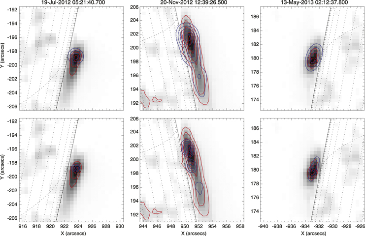
Figure 5. Zoomed view (15'' × 15'') around the stronger flare ribbon shown in Figure 3: The top row shows RHESSI Clean images reconstructed with the nominal highest resolution of 2 3 FWHM. The RHESSI images shown below are reconstructed with an artificially reduced point-spread function of 11 FWHM to roughly match the resolution of the HMI images. The same contours are shown for the RHESSI (blue) and HMI (red) images at 50, 70, 90% (for the more complex flare ribbon of the November 20 flare additional levels at 10 and 30% are shown).
Download figure:
Standard image High-resolution image
Figure 6. Radial cut through the main HMI source at the peak of each flare (no deconvolution of the HMI PSF has been applied): the pre-flare and the flare profile are given in black and red, respectively. The difference of these two profiles is given by the thick red curve. The blue curve is a Gaussian fit to the difference. The finite flux of the flare source around the limb is due to smearing out of the actual source by the HMI PSF function. For reference of the inflection point of the radial intensity profile, the derivative of the pre-flare is shown as a dashed curve. Plots are shown in linear (top) and logarithmic (bottom) scale.
Download figure:
Standard image High-resolution imageThe HXR (30–100 keV) centroid derived from the RHESSI data, using simultaneous sampling with the WL image discussed above, gives a radial distance of 946 ± 103 km. The error given is the statistical error derived from forward fitting of the RHESSI visibilities (e.g., Hannah et al. 2008); estimating the location from the different locations of the clean components gives consistent results (see Dennis & Pernak 2009). The emission perpendicular to the ribbon is unresolved at RHESSI's resolution of  (FWHM). The HXR footpoint is seen down to ∼20 keV, with the 20–30 keV image showing the same source morphology as at higher energies, but with a centroid being insignificantly higher by ∼33 km. At even lower energies, the thermal emission from the coronal flare loop dominates and emission from the footpoint source is lost in the limited dynamic range of the RHESSI images. The time evolution of the HXR emission reveals similar altitudes for the other 10 time intervals during the impulsive phase (Figure 2), with a trend toward slightly lower altitudes with time (about 300 km over the 7 minutes of the main HXR burst) that will be discussed below. The averaged difference of the WL and HXR altitude is 31 km with a standard deviation of 98 km. That the standard deviation is similar to the estimated statistical errors indicates that the error estimates are trustworthy. Within the statistical error, we conclude therefore that the HXR and WL are co-spatial.
A trend toward lower altitudes in time is observed for WL and HXR centroids (Figure 2, left bottom). This trend is most likely due to an apparent motion when the source positions change, but could also be due to an actual height change (see Figure 1). Besides this apparent motion in the radial direction, the northern source is also seen to systematically move along the limb in time with an average projected speed of ∼8 km s−1 (Figure 7). This apparent footpoint motion is generally thought to be due to the geometrical development of the reconnection process (e.g., Krucker et al. 2005). The northern ribbon structure seen in STEREO suggests that the ribbon direction deviates only slightly from the line of slight as seen from Earth. Nevertheless, it is unclear what the observed motion along the limb corresponds to. It could be due to separation of the ribbon as well as a foreshortened motion of a motion along the ribbon, or a combination of these two. Motions along the ribbons could produce the observed trend toward lower altitudes in time. The observed decrease by 300 km could be the result of a change in occultation heights by that amount. Starting exactly at the limb, this would correspond to a change by 29. This corresponds to a distance of about 40 Mm, and considering the 7 minute duration, a projected footpoint speed of 100 km s-1. This is a rapid footpoint motion speed, but not untypical for large flares (e.g., Metcalf et al. 2003; Yang et al. 2009). On the other hand, the estimated occultation height could be lower as the motion could start not right at the limb, and then a smaller angle could give the same effect. Despite all these unknowns, it is quite plausible that the decreasing altitude is an effect of footpoint motion. In such a case, the highest altitudes observed give the best estimates of the actual altitude with values around 900 km.
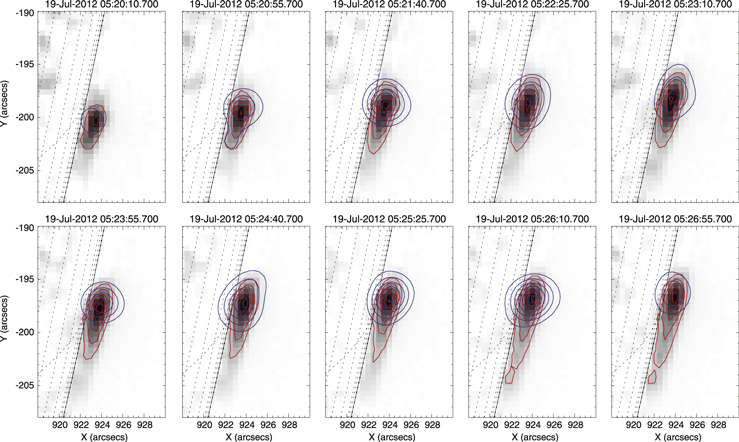
Figure 7. Time evolution of the northern footpoint of 2012 July 19 flare: the images as well as the red contours are both from HMI, while the blue contours are 30–80 keV HXR images. The RHESSI images are shown with the same time cadence and integration time as the HMI image. Both sources are observed to move along the limb toward the north.
Download figure:
Standard image High-resolution image
Figure 7 further reveals that the HXR sources outline the leading edge of the WL source, consistent with the picture that the energization of the WL emission is due to the non-thermal electrons that produce the HXR signal. The trail of the WL emission behind the newly flaring part of the ribbon could represent the cooling of the previously energized footpoint plasma after the HXR emission at that location has ended. This effect is most clearly seen in the close-up image shown in Figure 5 (left) where the HXR source is coming from the leading edge of the WL emission along the direction of motion. For on-disk flares, a similar behavior has also been observed (e.g., Isobe et al. 2007).
2.2. SOL2012-11-20T12:36 (M1.7)
SOL2012-11-20T12:36 (M1.7) has the smallest GOES flare class of the three flares presented here, but its non-thermal HXR peak flux is comparable to the flare with the largest GOES class (see Figure 2). The thermal flare loops are rather compact in size (Figure 3) and the impulsive phase is the shortest of the three flares, lasting only 2 minutes (Figure 2). A non-thermal coronal source cannot be detected for this flare, but the compact size of the flare together with the lack of significant occultation (see below) makes it much more difficult for RHESSI to observe a potential above-the-loop-top source.
From the Earth view, the two flare ribbons appear as a single elongated structure with length of ∼6 Mm along the limb. The STEREO images reveal that the flare ribbon geometry along the HMI/RHESSI LOS is short (∼1.1 Mm) and that the flare location as seen from Earth is between −01 and −13 on the rear side, with the best guess being around −05 for the stronger source. Projection effects therefore only influence the altitude estimates by <180 km. The STEREO observations indicate that the entire flare ribbon is seen from the Earth view (excluding the fact that low altitude emissions may not escape), potentially explaining the rather strong HXR emission of this flare relative to the other two events.
Figure 5 (center) shows the details of the WL and HXR ribbons during the peak of the impulsive phase. The altitude and radial extent of the WL and HXR at the peak time are again found to be co-spatial; the altitude and radial extent are given in Table 1. The best estimate for the flare altitude is similar to that of the first event with 799 ± 70 km, but the conservative upper limit is much better constrained with a value of ∼1000 km. Similar to the SOL2012–07-19T05:58 event, the footpoint emission is seen down to ∼20 keV with a 20–30 keV centroid being insignificantly higher (∼30 km) than the 30–100 keV centroid. The radial extent of the WL source is the smallest for all three events discussed in this paper, with a deconvolved size of ∼652 km. This could possibly be because projection effects are estimated to be least important for this event, or possibly because of its small spatial scale. The FWHM of the WL source is found to extend from an altitude of ∼475 ± 70 km to ∼1125 ± 70 km (projection effects could increase these numbers by maximal ∼180 km). The HXR centroids for the two images around the peak (the first WL frame has a shutter motion in the RHESSI data) are at 746 ± 51 km and 611 ± 33 km, respectively. The later time is slightly lower than the value derived for the WL, but not significantly so considering the errors.
2.3. SOL2013-05-13T12:36 (X1.7)
This flare is the first of two X-class flares occurring on the same day (e.g., Martínez Oliveros et al. 2014). It shows a large two-ribbon structure with a clear case of an above-the-loop-top HXR source. Systematic footpoint motion is also seen for this event, but the motion is more complex than in SOL2012–07-19T05:58. Detailed WL and HXR images of the strongest WL source are shown in Figure 5 (right). The STEREO images for this event are strongly saturated; the EUV emission is already saturated before the onset of the main HXR bursts. The best estimate for the WL source location is about 12 behind the limb for the strongest WL source shown in Figure 5. This corresponds to an occultation height of 150 km. For the worst-case estimate, however, the source could be as far behind as −41 (∼1800 km occultation). Hence, a source at the far of the ribbon at an altitude of 800 km as seen for the other events would be occulted. The best estimate for the WL source height is similar to the other two events, but the upper limit is much less constrained (Table 1). The HXR centroids (emissions above ∼28 keV are dominated by footpoints) are again found to be co-spatial with the WL emission.
3. SUMMARY AND DISCUSSION
We have analyzed three flares with WL and HXR footpoint sources seen above the limb to study the location of energy deposition by flare-accelerated electrons (HXR sources) relative to the location of efficient radiative losses (WL sources). For all three events, the WL and HXR centroids are observed to be co-spatial and appear about 800 km above the photosphere (∼300–450 km above the limb height). While the HXR sources are unresolved in the radial direction, the FWHM of the WL emission is ∼652 km for the event with the narrowest radial extent, and around 850 km for the other two.
The observed radial extent does not reflect an actual (local) source thickness. If the source is spatially extended in the east–west direction, occultation effects will smear out the source in the radial direction making it appear wider. However, even if occultation effects are not important, the source could consist of unresolved individual field lines with different density structures in the chromosphere that make the source appear to be extended in the radial direction compared to a model with a single density. Hence, the physical magnitude of the radial extent is difficult to estimate making a comparison with model prediction ambiguous.
The observed radial heights of the sources also do not necessarily represent actual radial heights for three reasons that we can identify: projection effects due to the position of the footpoint away from the exact limb position as seen from Earth, projection effects due to the superposition of distributed sources along the LOS, and the absorption of emission along the LOS. While absorption potentially hides emission from lower altitudes, projection effects go in the other direction with the actual values being potentially higher than what is observed. STEREO images reveal that for SOL2012-11-20T12:36 projection effects are smallest given an upper limit of 979 ± 70 km for the actual radial altitudes of the WL emission and 926 ± 51 km for HXR source. For the other two events the uncertainties are significantly larger (see Table 1). Due to absorption, the existence of additional emission from lower altitudes such as reported by Martínez Oliveros et al. (2012) cannot be excluded with these observations. Preliminary results from our ongoing HMI/RHESSI statistical study reveal that the above-the-limb events reported here have significantly lower ratios of WL to HXR flux than on-disk events. The lower ratios are at least partially due to limb darkening, but could potentially indicate the existence of a hidden WL source at low altitude. Future publications will look into this issue. In any case, our three limb flares point to source altitudes significantly above the limb height. For SOL2012-11-20T12:36, the estimated peak location at 799 ± 70 km together with the radial FWHM extent of ∼652 km indicate that the WL sources is below 50% of the peak value at the inflection point around 350 km. Hence, at least for SOL2012-11-20T12:36 the observed source around 800 km could be a real maximum in height. However, a more detailed theoretical study of the optical depth as a function of height above the photosphere needs to be done to better understand what can be observed for sources right above the limb. Such a study is planned to be published at a later time. Additionally, there is the uncertainty on altitude for the case the flare footpoints occur within a Wilson depression. In such a case, the altitude could appear a few hundred kilometers lower than given here. In summary, the observed radial profiles are not easy to translate into absolute altitude. However, the result that the WL and HXR sources, at least the visible parts, are co-spatial, appears to hold in any case.
3.1. Implication for the Thick-target Model
Compared to the expected theoretical altitude from the thick target model (see the introduction section), the observed values reported in this paper are rather low, despite being well above the altitude of the sources in SOL2011–02-24 analyzed by Martínez Oliveros et al. (2012). The observed altitudes would correspond theoretically to values derived from strongly beamed models using a low density model (Battaglia & Kontar 2012), in a vertical field orientation. However, a statistical study of the albedo components of solar flare footpoints by Dickson & Kontar (2013) indicates that strong beaming is not realized, and that the HXR emitting electron distribution is instead rather isotropic. This is also consistent with the lack of HXR directivity from the limited sampling afforded by stereoscopic observations (e.g., Kane et al. 1998). For weak beaming, the expected source altitude is significantly higher than for the strongly beamed model with values around 1500 km. For SOL2012-11-20T12:36 such values can be excluded while, for the other two events the uncertainties are too large for such a statement. A possibility of making our observations consistent with a weakly beamed thick target model is to introduce a re-acceleration process within the chromospheric HXR source. In these models the additional acceleration makes the electrons penetrate deeper into the chromosphere than in the nominal thick target beam model (e.g., Varady et al. 2014). However, the process of re-acceleration is hypothetical at the present stage. In conclusion, these observations do not exclude the thick target model, but they do restrict its allowed parameter space, particularly in terms of the density in the flaring footpoint (low densities).
3.2. Implication of Co-spatial HXR and WL Sources
On-disk events typically show that the horizontal extent of WL and HXR footpoints are also co-spatial (e.g., Krucker et al. 2011; Martínez Oliveros et al. 2012). Together with the findings for the three events that are co-spatial in radial directions, these results strongly suggest that WL and HXR footpoint emissions come from the same volume, independent on the issues of projection effects, absorption, and Wilson depression. This indicates that the collisional losses of  keV electrons are somehow directly related to the WL emission (a rough upper limit of 30 keV is used here as the lower limit of the footpoint HXR emission of ∼20 keV is typically produced by electrons above 30 keV). As the WL emission is thought to be produced by rather low-temperature plasma (
 K), the energy deposition by the HXR-producing electrons above 30 keV seems mostly to result only in weakly heated chromospheric plasma without producing the hot (>1 MK) plasma that could produce the hot (typically 10–30 MK) flare loops through the process of evaporation. The energy in flare-accelerated electrons above 30 keV is therefore directly radiated away at optical and UV wavelengths from within the HXR source. If there were additional emissions from even lower altitudes that are not able to escape, this argument would still hold as lower-altitude emissions are not expected to be at higher temperatures.
Heating by electrons at the low-energy end of the accelerated electron spectrum (i.e., at the electron energies that are not contributing to the 30–100 keV images analyzed in this paper) that are potentially stopped at higher altitudes could still produce hot (∼1–20 MK) footpoint emission, as has been previously reported (e.g., Hudson et al. 1994; McTiernan et al. 1994; Mrozek & Tomczak 2004; Graham et al. 2013; Tian et al. 2014). The centroid position as a function of energy indeed generally shows higher altitudes for lower energy (∼20 keV) HXR emissions by a few hundred kilometers (e.g., Kontar et al. 2008). This is also seen for the events discussed here, but the observed difference with values around 30 km is not significant considering to the uncertainties. Observations at even lower HXR energies (<20 keV) are generally dominated by thermal emission from the coronal flare loops, and non-thermal emission from footpoints at such energies are generally lost in the limited dynamic range of RHESSI. Nevertheless, future efforts should focus on finding limb events with relatively weak thermal emissions to potentially get images of non-thermal footpoints at lower energies as well. Candidates for such events could be flares with prominent HXR bursts right at the onset when the thermal emission is still relatively faint (e.g., Sui et al. 2007). Despite the fact that all three events discussed here show co-spatial HXR and WL sources, co-spatial sources might not necessarily exist for all flares. Some flares do not show detectable WL emission, and for such events >30 keV could potentially heat chromospheric plasma to coronal temperatures. A statistical study including all HMI and RHESSI flares is currently under preparation to investigate questions of this kind.
The work was supported by Swiss National Science Foundation (200021-140308), by the European Commission through HESPE (FP7-SPACE-2010-263086), and through NASA contract NAS 5-98033 for RHESSI.