


ABSTRACT
We present a detailed study of the complete evolution of a coronal mass ejection (CME). We have tracked the evolution of both the ejecta and its shock, and further fit the evolution of the fronts to a simple but physics-based analytical model. This study focuses on the CME initiated on the Sun on 2012 July 12 and arriving at the Earth on 2012 July 14. Shock and ejecta fronts were observed by white light images, as well as in situ by the Advanced Composition Explorer satellite. We find that the propagation of the two fronts is not completely dependent upon one another, but can each be modeled in the heliosphere with a drag model that assumes the dominant force of affecting CME evolution to be the aerodynamic drag force of the ambient solar wind. Results indicate that the CME ejecta front undergoes a more rapid deceleration than the shock front within 50 R☉ and therefore the propagation of the two fronts is not completely coupled in the heliosphere. Using the graduated cylindrical shell model, as well as data from time-elongation stack plots and in situ signatures, we show that the drag model can accurately describe the behavior of each front, but is more effective with the ejecta. We also show that without the in situ data, based on measurements out to 80 R☉ combined with the general values for drag model parameters, the arrival of both the shock and ejecta can be predicted within four hours of arrival.
Export citation and abstract BibTeX RIS
1. INTRODUCTION
Coronal mass ejections (CMEs) and their counterpart interplanetary coronal mass ejections (ICMEs) are a major driver of space weather effects at the Earth. A CME is an eruption of magnetized plasma from the Sun. Extreme cases of CMEs show speeds over 3000 km s−1 and carry as much as 1032 erg of energy (Howard et al. 1985). An ICME at the Earth will cause geomagnetic activity (Gosling et al. 1991; Zhang et al. 2003; Zhang et al. 2007). When its magnetic field has a strong component in the southward direction, which makes it oppositely aligned to the field of the Earth, an ICME will cause magnetic reconnection along the magnetopause, opening the magnetosphere and allowing solar wind energy inside. These geomagnetic storms can affect and damage a wide array of technological systems, including satellites, power grids, and GPS navigation systems, as well as endangering astronauts in space. Therefore, besides being scientifically intriguing, the ability to understand the processes governing CME evolution and to predict an arrival at Earth is crucial to our increasingly technological society (Schwenn 2006; Pulkkinen 2007).
Before the launch of the Solar Terrestrial Relations Observatory (STEREO) Mission in 2006, attempts to study CME evolution were primarily limited to two sets of data—white light and extreme ultraviolet (EUV) observations near the Sun and in situ data measuring CME signatures in the solar wind. The Solar Heliospheric Observatory (SOHO), launched in 1996, had the Extreme ultraviolet Imaging Telescope for observing the low corona in four EUV wavelengths and the Large Angle Spectral Coronagraphs (LASCO), which could measure the heliosphere out to 32 R☉ in white light. CMEs further out in the heliosphere were largely unobserved, except in radio interplanetary scintillation (IPS) observations (Manoharan et al. 2001) observations and white light data from the Solar Mass Ejection Imager (SMEI; Jackson et al. 2004). Tappin (2006) used SMEI data to show the deceleration of a CME out to five AU and introduced the Snow–Plough model, which has the CME slowing down due to conservation of momentum and the accumulation of solar wind plasma.
STEREO improved upon the available data with the Sun Earth Connection Coronal and Heliospheric Investigation (SECCHI) suite of instruments, which provide a continuous view of Thomson scattered white light from the Sun to the Earth (Howard et al. 2008). In addition, the STEREO mission is composed of two almost identical spacecraft in near 1 AU orbits around the Sun. This allows for unprecedented stereoscopic imaging of the Sun and heliosphere and three-dimensional tracking of CMEs all the way from the Sun to the Earth. Many works have already been performed using SECCHI data to study the velocity of CMEs in the heliosphere (Wood & Howard 2009; Lugaz et al. 2009; Rouillard et al. 2009; Tappin & Howard 2009; Möstl et al. 2009; Liu et al. 2010; Poomvises et al. 2010; Byrne et al. 2013; Colaninno et al. 2013; Mishra & Srivastava 2013), but most of these attempts have focused on just one of the CME fronts.
Many CMEs have two distinct fronts. When a CME is moving faster than the local Alfvén speed, a shock wave will be formed ahead of the CME ejecta. Between this shock wave and the ejecta will be the sheath region of compressed solar wind plasma. It has been found that, in addition to the ICME ejecta itself at the Earth, geomagnetic storms can be also caused by a CME driven shock sheath (Zhang et al. 2008). Studies show that, on average, the shock sheath region contributes about 30% of energy input into the magnetosphere, and for some events, this percentage can be more than 80%. If the compressed magnetic field of the sheath region between the CME driver and the shock has a strong southward component, it is possible for the shock sheath alone to be the structure through which the magnetic reconnection is driven. Shocks are also known to accelerate solar energetic particles (SEP), which are among the most urgent space weather concerns (Reames 1999; Gopalswamy et al. 2002; Kahler & Reames 2003). Shock measurements may also become more important as Kim et al. (2012) demonstrate a method of determining the magnetic field strength of the corona. It has previously been shown that in addition to having obvious structures in in situ solar wind data, shocks of sufficient strength can also be seen in white light images (Ontiveros & Vourlidas 2009; Maloney & Gallagher 2011; Bemporad & Mancuso 2010; Vourlidas et al. 2003). It is then possible to use SECCHI to track both the CME ejecta and the shock it drives through the interplanetary space and relate it to in situ signatures at the Earth.
To prevent any confusion, the following terminology will be used to describe the CME and ICME structure throughout the rest of this paper:
The ejecta, driver, or flux rope refers to the same CME structure, possibly a magnetic flux rope, that erupts from the corona. In the classical "three part" CME structure (Illing & Hundhausen 1985), this area is considered to be the cavity. The ejecta front refers to the region of enhanced emission immediately surrounding the ejecta.
The shock front is the outermost front seen in images. It is a shock wave caused by a fast CME as it travels through the interplanetary space. In images it is seen as a faint and diffuse region in front of the ejecta. Throughout the paper, we will try to avoid using CME front, since it could be interpreted either as the ejecta front or the shock front.
In between these two fronts, the sheath region is an area of accumulated solar wind material that is highly dense with varying size, and can contain an enhanced but complicated magnetic structure.
CME will hereafter refer to the entire structure, including the ejecta, sheath, and shock front as defined above, whereas ICME will refer only to CME signatures as seen in situ (e.g., with the Advanced Composition Explorer (ACE) spacecraft).
The different in situ signatures that will be discussed are the shock, which is seen as a sharp increase in magnetic field strength, velocity, and density (Jackson 1986), and the sheath, which is the high density region between the shock and the CME driver. The CME driver often appears as the classical magnetic cloud structure: a rotating magnetic field, a temperature that is significantly lower than expected based on the velocity, and a region where magnetic pressure is significantly larger than thermal pressure, which can also be considered a region of very low β (Zurbuchen & Richardson 2006). Magnetic clouds have long been regarded as magnetic flux ropes (Burlaga et al. 1981; Lepping et al. 1990).
Initially, the ejecta is relatively small and has the highest density, so it can be very bright in white light images. Conversely, the sheath will initially be very faint, as it is comprised of accumulated solar wind plasma in front of the CME driver. As the CME propagates, these brightness intensities will reverse relative to one another, as the CME will continue to expand as it propagates. This will decrease its density, but the shock will accumulate more and more plasma and therefore gain brightness, or at least, lose brightness less quickly than the ejecta.
This study features a complete tracking of the evolution of both the shock and ejecta fronts and a comparison of the two, with an attempt to fit the evolution of the fronts to a simple but physics-based model. The rest of the paper is organized as follows: Section 2 will outline the methods used to track and measure the CME and the CME driven shock and the means by which meaningful data is extracted from the measurements, as well as the physical assumptions that produce the model we use to fit the two fronts. Section 3 presents the data for one particularly well-observed event on 2012 July 12. Section 4 will discuss the applications of these methods and potential impacts for space weather prediction.
2. METHODS
2.1. Observations
On board the STEREO spacecraft, SECCHI contains five separate instruments: the Extreme Ultraviolet Imager measuring EUV radiation at four wavelengths; two coronagraphs, COR1 and COR2, which observe white light ranging from about 1.4–4 R☉ and about 2.5–15 R☉, respectively; and two Heliospheric Imagers, HI-1 and HI-2, which have ranges of about 15–84 R☉ and 66–318 R☉, respectively. The Heliospheric Imagers, like the coronagraphs, observe Thomson scattered white light. By combining observations from each instrument, a CME can be tracked continuously from its eruption in the low corona into the heliosphere (Howard et al. 2008).
The primary data sets used for this work are the COR2, HI-1, and HI-2 instruments on board the two STEREO spacecraft, as there is an SEP related data gap in SOHO LASCO data for much of the propagation. In situ data was obtained from the ACE, a spacecraft at the L1 point that has instruments for measuring both the magnetic field (Magnetometer) and the properties of the plasma (Solar Wind Electron-Proton and Alpha Monitor) of the solar wind.
2.2. Obtaining Height Measurements
Different methods and models for extracting CME height data from STEREO have been developed (Tappin & Howard 2009; Lugaz et al. 2009; Thernisien et al. 2009; Liu et al. 2010; Mishra & Srivastava 2013). For the purpose of studying the evolution of the shock and CME ejecta fronts in this paper, two different methods were used.
The first is a forward modeling technique that uses the graduated cylindrical shell (GCS), or croissant geometric model, utilizing the raytrace code developed by Thernisien et al. (2006, 2009). A demonstration of the model is shown in Figure 1. This model involves taking a cylindrical croissant defined by six free parameters and superimposing it upon images from multiple spacecraft at once; the parameters are chosen such that the model image best matches the observed images from multiple view points. These parameters are the direction of propagation (longitude and latitude), the leading edge distance of the tracked feature from the Sun, the half angle width of the shell, the tilt angle of the flux rope central axis orientation, and the ratio between the major and minor radius of the flux rope (aspect ratio). Making the assumption that the other five parameters are roughly constant as the CME propagates, the leading edge height can be used to determine a height profile of the CME with time. Performing a numerical derivative of this data can then yield a velocity.
Figure 1. Model fitting of CME ejecta and shock front. Images at 17:54 UT on 2012 July 12 from STEREO A COR2 (left) and STEREO B COR2 (right) are shown, along without (top) and with (bottom) the raytrace mesh. The green mesh shows the GCS fitting to the CME ejecta, whereas the red mesh shows the spheroid fitting to the CME shock front. A supplemental movie showing the CME and the mesh is provided.
(An animation and a color version of this figure are available in the online journal.)
Download figure:
Video Standard image High-resolution imageThe geometric structures utilized in the raytrace code are idealized structures, and for some events it can be difficult to match the model to the data. For the July 12 event, there is a bright feature that is not being fit as part of the ejecta, as seen in Figure 1. As can be seen more clearly in Figure 2, this feature is not part of the cavity structure of the CME ejecta, but instead is likely a streamer disturbed by the CME shock sheath region.

Figure 2. Tracking CME ejecta using the direct image (left) and the shock front using the difference image (right). Images from STEREO A COR2 at 17:54 UT on 2012 July 12 are used as an example. The image on the left is a base-ratio direct image where the flux rope or ejecta (outlined by the blue line) is better shown. The bright feature at the bottom of the ejecta outside the blue line is believed to be a disturbed streamer. The shock front is better seen in the running difference image in the left (demarcated by the red line).
Download figure:
Standard image High-resolution imageIn addition to the croissant-shaped flux rope, there is also a spheroid shock model in the code, with six free parameters as well. Some of these, also in the flux rope model, are propagation direction (longitude and latitude), tilt, and height. The other two parameters, ε and κ, control the major and minor axis of the spheroid.
As this work is focusing mostly on the shock and ejecta leading edges, less attention was paid to ε and κ, which are more important to the detailed three-dimensional shock geometry. However, both features can be tracked in such a way that the heights along the leading edge can be tracked, leading to an understanding of the independent evolution of each front, as well as the size of the sheath region between them.
In order to track the different features into the heliosphere, it is important to process image data in such a way that both features are distinguishable. In white light observations, the CME flux rope is best seen in direct images, which are made through a base-ratio technique where an average background is used as the denominator, while a particular image is numerator in the ratio; a direct image allows the bright features of the flux rope and the internal structure to be seen. On the other hand, to make the shock front and sheath more clear, a running-difference image subtracting the previous image from the current one is more useful, as the outermost features corresponding to the shock are often faint and diffuse. An example of both types of images and the different features is seen in Figure 2.
While success has been shown using the raytrace model to track CMEs (Thernisien et al. 2009; Poomvises et al. 2010; Nieves-Chinchilla et al. 2012), another method was sought as a complement to the raytrace measurements. The height measurements can also be made using so-called jmaps (Sheeley et al. 1999), which are stack plots of image slices along a given position angle from one spacecraft that provides plots in terms of elongation angle versus time. However, due to various observational effects (Howard & Tappin 2009; Lugaz et al. 2009), getting the true de-projected heights in distance from the Sun from jmaps is not as easy as just converting the elongation angles to a distance. There are different methods for deriving true distances. The simplest of these, so-called fixed-φ is given by
where ε is the elongation angle of the object being tracked, as determined from the jmap, and φ is the direction of propagation of the CME relative to the observer, and Dobs is the distance from the observer to the Sun.
Fixed φ has been shown to be useful near the Sun, but as the CME propagates out it begins to greatly overestimate the leading edge position (Rollett et al. 2012). For this reason, the harmonic mean method was also used. Of all methods utilizing single spacecraft observations, Mishra & Srivastava (2013) found the harmonic mean method to be the most successful. The equation for this method is
This equation represents the harmonic mean between fixed ϕ and the Point-P method, given by

which is the simplest, and most inaccurate, method of deriving true heights from single-spacecraft observations. While it is inaccurate, as Point-P tends to underestimate the true heights, it helps provide a correction for the geometric effects of fixed ϕ (Lugaz et al. 2009).
While most work in the past has attempted to fit the data to provide the best estimation of the direction of propagation, this study is different in that the propagation direction from raytrace was used, allowing for a straight-forward calculation of leading edge distances. Using the same direction of propagation as raytrace could introduce bias in the jmap data, however this should not be a significant issue because the direction of propagation has a relatively small error in the stereoscopic-based raytrace method. The jmaps used along the leading edge position angle are presented in Figure 3, along with the measurements used for the shock.

Figure 3. Jmaps of the 2012 July 12–14 CME for each STEREO spacecraft along the propagation angle as measured by the raytrace method. The CME is clearer in STEREO A. The bright density enhancement is considered the sheath region of high density. The edge leading this sheath is considered to be the shock front. The red crosses show the elongation measurements used for the shock obtained from each jmap.
Download figure:
Standard image High-resolution imageThe jmaps from STEREO A and B shown in Figure 3 both show a bright feature beginning in the COR2 field of fiew (FOV), which remains into the HI-1 FOV. The leading front of these two was taken to be the shock front, while the brighter front trails behind. Judging from the appearance of the front in the HI-1 FOV, these fronts are part of the same overall structure, which continually becomes more diffuse. For this reason, the outermost front is the one that was tracked.
These methods solved the problem of how to convert measurements from jmap elongation angles into heights, but there was still the issue of how to interpret the jmap data for the purpose of studying the separate fronts of the CME. Rouillard (2011) relates bright features in jmap data to density enhancements in situ, which makes practical physical sense because the higher the density of a region, the more light will be Thomson scattered and the brighter these areas will be in white light images. Therefore, following this logic, the bright features in the white light images will be taken to be the sheath region, which will have the highest density. The shock front will be the leading edge of the bright feature in the jmap.
In the coronagraph FOV near the Sun, the interpretation of the bright features is different. Due to the observational fact that the CME ejecta is brighter than the shock near the Sun, the assumption in the previous paragraph may be invalid. The HI-1 data is where the two fronts begin to separate themselves more distinctly, so this is more important, and in the majority of the HI-1 data the sheath gains more optical significance.
While this general assumption of the fronts should be valid, there is one more significant issue that should be considered with this interpretation of jmap data. Jmaps are constructed using running difference images. In the case of the shock front, this should not matter, as the shock front is generally traveling into an empty region of space and can be well seen in a running difference image. However, if the sheath region is larger than the distance traveled by the shock front between two images, the shock region that gets subtracted out from the previous image will remove the back of the sheath and leave a dark void. In a jmap it is possible that this void would be interpreted as the ejecta, when it is actually an observational artifact. Therefore with the jmap data, the focus will remain on the shock front.
In addition, errors are also introduced in jmaps because generating a clear and coherent image of the different images stacked together requires pre-processing and smoothing of the images. While this creates an image that is easier to interpret, it is possible that data will be smoothed over. Between these issues and the fact that a jmap only takes data from one vantage point, as opposed to the three views in raytrace, the raytrace is considered the more accurate measurement (but limited to within HI-1 FOV), although all data sets are useful.
2.3. Modeling the Data
With both the GCS model and jmap interpretation to get height time data, a method is needed to obtain velocity profiles for each front. As shown in Byrne et al. (2013), simply taking a numerical derivative of the measurements is not a reliable way to get an accurate result for the CME velocity. Typically, to get data that makes sense using a numerical derivative such as this, smoothing and other manipulations must be performed, introducing more errors. Error is also caused by the non-uniform time cadences of the different instruments and fields of view. Given all this information, it is typically more reliable to choose a certain functional form to fit the data in the height time space and analytically derive this function to obtain a velocity and acceleration.
For this work, the model used to fit the height time data is the drag model (Vršnak et al. 2013), which is a semi-empirical model that assumes that after the initial CME acceleration, magnetic forces are no longer a significant factor in governing CME evolution and aerodynamic drag is the primary force acting on the CME. The equations of motion in the drag model begin with an assumption of a quadratic acceleration and can be analytically integrated to produce velocity and height as a function of time. The equations of motion are

where v0 is the initial CME speed, vsw is the upstream solar wind speed, r0 is the initial CME height, and γ is the drag parameter that controls the rate at which the CME reaches the solar wind speed. For our work with these equations, we are assuming that both γ and vsw are fixed throughout the CME propagation. Both of these parameters are actually functions of radial distance, especially lower in the corona as the solar wind gets accelerated and the CME begins to expand (Vršnak et al. 2004). This also assumes the entire CME is encountering one static solar wind regime, which may be very incorrect for some events. Approximating γ and vsw as constants allows us to use the equations above, and fit them as a static parameter.
For theses fittings and with our assumptions, most of the parameters can be determined with just a little information. The initial CME speed and height can be well constrained from observations. vsw is obtained by taking the average upstream speed of the solar wind eight hours ahead of the arrival of the CME at ACE. For events that experience drastically different solar wind regimes, the assumption that this solar wind speed is representative of the entire upstream regime may introduce significant error, but for most events it should work. This leaves the only totally unknown parameter in the model as γ, the drag parameter. Assuming this is a fixed value throughout propagation, it can be easily fit using the height measurements to get the height time profile.
3. RESULTS
3.1. The 2012 July 12 CME
Applying these methods to the 2012 July 12 CME, both the shock front and ejecta front were tracked. Extreme ultraviolet images and GOES X-ray data show an eruptive X1.4 flare originating from AR 11520 (S17° W08°) with an X-ray peak around 16:45 UT on the 12th. This same active region produced a number of strong flares and CMEs, including the July 23 backside CME, which was considered the fastest CME observed in the STEREO era (Liu et al. 2014). The CME was well observed by COR2 and HI-1 in both STEREO A and B and can also be seen in HI-2, as shown in Figure 4. However the associated SEPs limit the SOHO LASCO data to just a few frames between the eruption and the CME passing beyond the C3 FOV. Both heliospheric imagers observe the event, allowing it to be tracked out to about 80 R☉ before the different structures become too diffuse and faint to be clearly identified.
Download figure:
Video Standard image High-resolution imageFigure 4. Images from STEREO B (left) and A (right) from COR2 at 17:24 UT on 2012 July 12 (top), HI-1 at 21:29 (middle), and HI-2 at 10:09 on 2012 July 13 (bottom). A supplemental movie showing the propagation in the different fronts is provided.
(Animations (a and b) of this figure are available in the online journal.)
Download figure:
Video Standard image High-resolution imageThe ICME was observed in situ by ACE as seen in Figure 5. The shock is seen as a spike in the magnetic field, velocity, and temperature at approximately 17:15 UT on July 14. Curiously, the density does not show a strong jump indicative of a shock. The sheath lasts for almost 14 hr until around 07:00 UT on the 15th, when the magnetic cloud structure of the flux rope arrives. As is often the case, the boundaries of the magnetic cloud are more ambiguous than those of the more clearly defined shock. In this case, the main signature used to define the flux rope as seen in Figure 5 was the lowered proton temperature, compared to expected temperature (Lopez & Freeman 1986; Richardson & Cane 1995) and the drop in plasma-β. There is certainly room for the interpretation of the arrival of the flux rope, but changing the exact arrival slightly should not have a significant impact on the results.
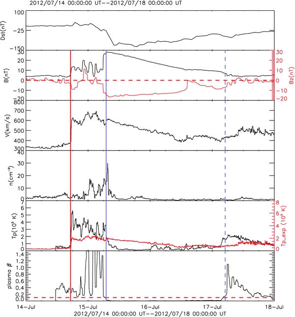
Figure 5. Solar wind data measured by ACE between 2012 July 14 and July 18. The shock onset is denoted with the red line, the ejecta onset with the solid blue line, and the passing of the ejecta with the dotted blue line. Plots from top to bottom show the Dst index, total magnetic field, and the z component of the magnetic field (red), total velocity, density, temperature, and the expected temperature (red) based on the velocity, and the plasma β.
Download figure:
Standard image High-resolution imageThe flux rope initially shows a strong southward magnetic field with a maximum strength of 16.7 nT. The total field has a peak of 28.4 nT, which gradually declines as the flux rope passes the spacecraft. The x, y, and z directions of the magnetic field all show rotational signatures representative of the helically twisted field lines of a flux rope. The velocity shows gradual decline, a sign of an expanding flux rope and as expected, low density and temperature are also shown in the magnetic cloud. The ICME causes a strong geomagnetic storm with a Dst peak of −127 nT on the 15th that lasts for many days before Dst recovers.
To keep the raytrace data consistent, only one of the six parameters that was altered from time step to time step was the height, the other five were held constant for each measurement. While this certainly introduces errors, as the CME will change in time due to internal forces and interaction with the ambient solar wind, it is assumed that these changes are not significant over the short timeframe (less than one day) for which the raytrace measurements were carried out. For this event, the five constant parameters are a latitude of −8 9, a heliographic longitude of 03, tilt angle of 581, half angle width of 254, and aspect ratio of 0.37. The croissant shape used is comparable to the same model presented in Möstl et al. (2014), which also fit the initial propagation longitude to be within 1 of the Sun–Earth line.
The propagation direction was chosen by first locating the source region of the event in EUV coronal images. All the parameters were then varied until they provided the best match to the images in the coronagraph/heliospheric imager data for as long as the CME is clearly visible. Since the entire CME structure is not visible in the HI-1 FOV, most of the parameters must be determined while the CME is in the COR2 FOV, and by the time the CME passes beyond this FOV, only the height can be determined.
The propagation direction for this event indicates that is a nearly perfect event for comparing remote-sensing observations with in situ data, as both longitude and latitude are within 10° of the Sun–Earth line. The jmaps used for measurement were taken along the same position angle as the leading edge of the CME, so a direct comparison with the height profile from the raytrace method could be made. For predictive purposes, the CME evolution along the equatorial plane is more relevant than that along the CME leading edge, but for this particular event we found that the propagation direction of the CME was close enough to the Sun–Earth line that this distinction was not significant.
3.2. Drag Model Fitting
The data in Figure 6 show the raytrace measurements as well as the in situ arrival times with the drag model fittings plotted with them. The associated velocity and acceleration profiles are shown in Figure 7. The parameters of the fitting are shown in full in Columns 1–4 of Table 1. The top two rows show the flux rope and shock parameters, respectively, for the full fitting with the in situ data point included. Rows 3 and 4 show the parameters for a fitting without the inclusion of any in situ data that would be more predictively useful. Also presented in Table 1 is the average in situ velocity of each feature (Column 5), the velocity of the drag model at the point it reaches 1 AU (Column 6), and the difference in time between the actual and modeled in situ arrivals (Column 7).

Figure 6. Raytrace measurements (black) for both the shock (stars) and ejecta (crosses), as well the ACE in situ measurements (gold). The least-squares drag fittings of the data are included as the dashed red (shock) and solid blue (ejecta) lines.
Download figure:
Standard image High-resolution image
Figure 7. Top plot is the velocity profile for the fitted drag model for both shock (red dashed line) and ejecta (blue line). The bottom plot is the acceleration of the model.
Download figure:
Standard image High-resolution imageTable 1. The Drag Fitting Parameters of the Two Front and the in situ Parameters from ACE
| γ | V0 | Vf | R0 | In situ Velocity | Drag Model | ΔT | |
|---|---|---|---|---|---|---|---|
| (km−1) | (km s−1) | (km s−1) | (RS) | (km s−1) | (km s−1) | (hr) | |
| Flux rope | 3.09e-8 | 1316.5 | 353.7 | 4.29 | 487.7 | 477.9 | .69 |
| Shock | 1.47e-8 | 1259.4 | 353.7 | 8.69 | 608.3 | 625.5 | .89 |
| Flux rope prediction | 6.15e-8 | 1423.8 | 500 | 4.29 | 487.7 | 571.5 | −3.8 |
| Shock prediction | 4.77e-8 | 1548.6 | 500 | 8.69 | 608.3 | 598.9 | 4.2 |
Notes. The ACE velocities are the average over the full in situ time range for both the shock-sheath region and the flux rope.
Download table as: ASCIITypeset image
The drag model, using a final asymptotic speed for both fronts of 353.7 km s−1, is still able to reproduce the speed of the shock and the flux rope as observed in situ quite well, even though at 1 AU both fronts were still in the process of decelerating. This is a sign that the drag model is able to accurately capture both the flux rope and shock propagation using height-time measurements near the Sun and one in situ data at L1. More events will now have to be studied to determine the physical significance of the drag parameter, and how it may be predicted for the creation of an empirical space weather forecasting tool, with a more physical basis than other purely empirical models (Gopalswamy et al. 2005; Kim et al. 2010; Wood et al. 2012).
Our drag parameter, γ, for each front, 1.47 × 10⁻⁸ and 3.09 × 10⁻⁸ km−1, is similar to those derived theoretically in Vršnak et al. (2013), although more work must be done to understand the parameters in the data that might be used to successfully predict this important value. However, the great difference in the two separate γ values is an illustration that the two fronts, while following a similar evolution, are still separate and independent.
To perform an analysis of the error, we assume that the GCS method for the flux rope in COR2 has an error of ±.5 R☉, with the total 1 R☉ error representing about 3% of the total FOV of the instrument. Since the shock is often diffuse and difficult to see in COR2, we double this to ±1 R☉. For both fronts in HI-1, we use an error of ±2.5 R☉, which is a total error of about 7% of the HI-1 FOV. The increase in error in HI-1 is due to the increase in the ambiguity of the CME fronts further from the Sun, as well as the errors introduced by the image processing techniques required to bring the CME to the forefront as it propagates outward and expands and becomes less intense in the observations. For the drag-model fitting of the ejecta on the 2012 July 12 CME, this yielded a χ2-value of 12.5. With 23 degrees of freedom in the fit, this gives a p-value for the fit of.96. For the shock, the χ2-value was 28.4 with 22 degrees of freedom, for a p-value of just.16. This still indicates a decent fit. Examining the shock fit in Figure 6, it shows a good agreement further from the Sun, but under 30 R☉ the shock height is ahead of the model fit.
There are a number of possible explanations for this difference, with the possibility that the drag model is more physically descriptive for the flux rope traveling in the solar wind than it is for shock propagation. Still, the fit is good enough to provide an approximation of the shock propagation, and with the study of more events the model may be more adaptable to the shock front.
To confirm the raytrace measurements, they were compared with the jmap data, specifically along the shock, as seen in Figure 8. The ejecta was not compared due to the difficulty in reliably locating it in the jmaps. Both the fixed-φ and harmonic mean are included, rather than attempting to determine a point at which the latter begins to outperform the former. The data sets show qualitative agreement, at least before the fixed φ data begins to blow up, but there are still some significant discrepancies. The jmap data frequently under measures the shock compared to raytrace in the low HI-1 FOV (50 R☉), but later overestimates it. Instead of representing the drag behavior of the raytrace measurements where the CME starts fast and decelerates to the ambient solar wind speed, the jmap data shows a CME with a lower initial velocity that has a more linear profile.

Figure 8. Measured heights from the raytrace measurements (crosses) and jmaps, using both fixed φ (diamonds) and harmonic mean (stars). The jmaps were taken along the CME leading edge, as determined by the raytrace parameters. The observer distance used to get the heights was taken from the position of the STEREO spacecraft on 2012 July 13 at 12:00 UT.
Download figure:
Standard image High-resolution imageThe data are still close enough comparing the jmap with the raytrace measurements, thus it is fair to say they are generally consistent. However, we have much more trust in the raytrace measurement due to the number of different errors introduced in the jmap methods. Not only is the jmap just one two-dimensional projection rather than a stereoscopic reconstruction like raytrace, but there are also a number of image processing errors introduced, as well as the errors from determining where the shock boundary is on the jmap and the assumptions needed to convert elongations into height time measurements. The raytrace model also seems to align better with the in situ arrival point, which means we can be confident with our measurements.
Figure 9 shows the standoff distance, or the distance between the leading edge of the shock front and the leading edge of the ejecta front from the raytrace measurements. The standoff distance (black diamonds) is calculated by subtracting the measured ejecta front from the measured shock front. The line is the standoff distance from the models, which is taken by subtracting the ejecta drag fitting from the shock drag fitting. The solid vertical line shows the arrival of the shock at ACE and the dashed vertical line shows the arrival of the flux rope. The star symbol in the middle of the sheath timings at ACE shows the average in situ sheath size, as determined by integrating the ACE velocity data with time during the observed duration of the sheath. Error bars were obtained by doubling the error of the raytrace measurement in each FOV, since the standoff distance is a combination of two separate measurements. The model fitting matches reasonably well to the raytrace data in the HI-1 range, but there is significant deviation in the COR2 FOV. This is partially due to boundary effects of the parametric fitting. It might also be related to the fact that, nearer the Sun, the size of the standoff distance is small, compared to the error of the distance measurements. The model shows a standoff distance that has an exponential form in the early evolution, but for much of the later propagation, is roughly linear. This is supported by the observed sheath—integrating the velocity data at ACE over the sheath region, an average sheath size during the propagation of the sheath through the satellite can be obtained. The average in situ sheath was 43.5 R☉, or about 4–12 R☉ higher than the modeled sheath. This error could be an effect of either the model failing to fully capture the shock evolution, or an effect of the sheath being larger away from the CME nose; the location of the sheath from the ACE measurement is about 10 degrees from the nose of the CME. The model is representing the standoff distance right at the CME nose, whereas the in situ data is not.

Figure 9. Comparison between the measured standoff distance and the standoff distance of the shock and ejecta parametric models, as well as the standoff distance observed in situ. The solid vertical line shows shock arrival, the dashed line denotes ejecta arrival.
Download figure:
Standard image High-resolution image
Our model standoff distance results are in good agreement with Maloney & Gallagher (2011), who found a standoff distance of about 20 R☉ at 0.5 AU. Likewise, a model of standoff distance based on extrapolating fits to low corona measurements by Temmer et al. (2013) shows a standoff distance profile in the heliosphere that is very similar to our results, which also agree with typical in situ sheath sizes (Russell & Mulligan 2002).
3.3. Prediction
While the previous fittings with the drag model are useful for demonstrating the ability of the drag model to fit the CME ejecta and shock, those fittings are not particularly useful for a predictive purpose, because they include the in situ arrival of the fronts in the fitting. In order to use the model for prediction, the fittings must only contain information that can be obtained early in CME propagation. This means that the in situ arrival time and solar wind speed must be removed, which allows for testing the method as a predictive tool. Furthermore, even without prior knowledge of the solar wind speed and drag parameter, γ, predictions can still be improved by including limits on these values based on studies of different events.
Vršnak et al. (2013) show that a good range for γ is 1 × 10⁻⁸ to 1 × 10⁻⁷ km−1 and a solar wind speed of 300 to 500 km s−1 for a typical slow solar wind upstream of the CME, are useful for prediction. Using these limits on the parameters and fitting the raytrace measurements from eruption until 06:49 UT on the 13th, predicted arrival times could be calculated. The parameters are included in Table 1 for comparison to the parameters with the in situ arrival included.
Both the shock and ejecta front skew toward the maximum allowed solar wind speed of 500 km s−1, which is not surprising. The data being fit is all from within 80 R☉, at which point the CME is still in the process of slowing down and is traveling well above 500 km s−1. Without the in situ data point being included, no information on the propagation beyond this point is going into the model, so there is no way for the fitting to approach a more realistic final speed. The derived initial speeds are also higher for each front. Even with these higher initial and final speeds, the model still predicts the shock to arrive later than the actual in situ signatures. This is because of a significant increase in γ in both the shock and ejecta in the predictive fitting.
While the initial and final velocities of both structures are higher in the predictive fitting, with the higher amount of drag, the speed declines more quickly and the average speed of the propagation will be closer to the final speed. In the fittings including the in situ data, the drag is more gradual, leading to a higher overall average speed.
That the predictive fitting, which includes only data up to 80 R☉, has more drag is unsurprising. This is consistent with what was found by Poomvises et al. (2010) that most drag occurs within 50 R☉. This indicates that rather than using one static γ value, using a decreasing value with a stronger drag early in the propagation could be more physically accurate.
In terms of the success of the predictions, the shock prediction is about four hours late, and the ejecta prediction is about four hours early. Accordingly, the predicted shock velocity is lower than what is observed in situ, and the flux rope velocity is higher. This is an encouraging result for space weather prediction. It had an error of about 18 hr predicting the shock arrival for this same event, when a purely empirical model and far less data are used (Gopalswamy et al. 2013). The prediction also improves upon most of the methods used for this same event in Möstl et al. (2014) for the arrival of the shock, and compares favorably to the most successful prediction therein, the SSEF corrected model.
With the advantage of using data much further out into the heliosphere, we can greatly improve the accuracy of the prediction, with the caveat that even if the data could be accessed, processed, measured, and fit instantly, it would still provide a lead time of just about 30 hr on the prediction for this particular event. As more events are studied, it is our goal to have greater insight on the drag parameter, thus allowing us to predict the drag parameter with less data and have a model that combines the accuracy of the drag model predictions with the lead time of a more empirical model.
4. DISCUSSION AND CONCLUSIONS
While one event is not enough to form more definitive conclusions, the study of the 2012 July 12 event does provide a useful validation of the methods of studying CME kinematics and the basis for forming a useful predictive model. We have shown that it is possible, for events with a sufficiently strong shock, to track both the ejecta and shock independently well into the heliosphere using remote-sensing data from STEREO. In attempting to use different methods to obtain height time measurements of a CME in the heliosphere, we also present evidence that a three-dimensional stereoscopic reconstruction like raytrace is better than using a two-dimensional projection like a jmap. The raytrace method also has the advantage of distinguishing both fronts observationally. In attempting to provide a model to fit our measurements, we show success matching the drag model to our observations, with the understanding that the drag model may not fully capture the processes responsible for slowing the ejecta and especially the shock, particularly within 20 R☉, where our assumption of a static γ and vsw are less valid due to both the acceleration of the solar wind and the rapid change in CME density (decreases by r−3) relative to the ambient (decreases by r−2), which increases drag. For this particular event, the drag model does better with the parameters used on the flux rope. As more events are studied and measured, we can determine if the drag model is drastically more effective for the flux rope than the shock, if the shock needs its own separate model based on different parameters, and if we need to include a height dependence for γ and vsw. However, we do show that the analytical drag model can fit the measured shock data.
One interesting result is that the ejecta undergo a stronger deceleration than the shock in the early propagation. While the shock and the ejecta have a similar speed in the beginning, the shock speed is always higher than that of the ejecta afterward. Since the CME is driving the shock wave, the two fronts are necessarily coupled as the CME propagates toward the Earth. However, the fact that the ejecta undergo a stronger initial deceleration indicates that the propagation of the two fronts exhibits different kinematic behavior, but is not completely decoupled. That the ejecta decelerates faster than the shock matches a conclusion also found by Corona-Romero et al. (2013), using radio data rather than remote-sensing images to track the two separate structures.
This is a key finding and if confirmed by further study it will greatly improve our ability to predict the arrival of the two fronts separately at 1 AU, while gaining a better understanding of the physical processes that govern the evolution separately.
To extend this work in the future, more will be done to try to create a fully predictive drag model, where the initial speed can be found from observations, the solar wind speed can be obtained from data or from a data-driven numerical model, and γ can hopefully be uniquely defined for each event, based on current solar wind conditions either observed or simulated.
Once we have more input that can be used to constrain γ, the drag model fittings will hopefully be accurate without the in situ data point, making it predictively useful and allowing a maximum lead time on prediction. The ultimate goal is to be able to obtain an initial speed just after the CME erupts, and to immediately be able to predict the arrival of both fronts.
In order to create a predictive model, we will study many more events. Hopefully this will allow us to fully confirm our models and measurements, as well as gain important physical insight into the parameters, specifically drag, in the drag model, with the goal of being able to predict the amount of drag a CME will encounter. We will also compare both our measurements and the drag model with MHD simulations of CMEs to see if the same drag characteristics are observed in more complex models of the heliosphere.
This work is supported by NSF ATM-0748003 and NSF AGS-1156120. We acknowledge the use of data from the STEREO mission, the SOHO mission, and also the use of ACE data.