


ABSTRACT
The temperature dependence of the emission measure (EM) in the core of active regions coronal loops is an important diagnostic of heating processes. Observations indicate that EM(T) ∼ Ta below approximately 4 MK, with 2 < a < 5. Zero-dimensional hydrodynamic simulations of nanoflare trains are used to demonstrate the dependence of a on the time between individual nanoflares (TN) and the distribution of nanoflare energies. If TN is greater than a few thousand seconds, a < 3. For smaller values, trains of equally spaced nanoflares cannot account for the observed range of a if the distribution of nanoflare energies is either constant, randomly distributed, or a power law. Power law distributions where there is a delay between consecutive nanoflares proportional to the energy of the second nanoflare do lead to the observed range of a. However, TN must then be of the order of hundreds to no more than a few thousand seconds. If a nanoflare leads to the relaxation of a stressed coronal field to a near-potential state, the time taken to build up the required magnetic energy is thus too long to account for the EM measurements. Instead, it is suggested that a nanoflare involves the relaxation from one stressed coronal state to another, dissipating only a small fraction of the available magnetic energy. A consequence is that nanoflare energies may be smaller than previously envisioned.
Export citation and abstract BibTeX RIS
1. INTRODUCTION
The ability to carry out multiwavelength observations of active regions (ARs) has led to major advances in understanding how the coronal loops there may be heated. In particular, studies of so-called AR core loops (Warren et al. 2011, 2012; Winebarger et al. 2011; Tripathi et al. 2011; Schmelz & Pathak 2012; Bradshaw et al. 2012; Reep et al. 2013) have, for the first time, imposed serious and credible constraints on their heating. These AR cores were identified as being relatively simple locations, where the radiation from the corona was unlikely to be contaminated by that from the transition region (TR) at the loop footpoints (the "moss"), thus permitting a direct comparison with predictions from coronal heating models.
Using data from the EUV imaging spectrometer instrument on the Hinode spacecraft, with support from the Hinode X-Ray Telescope and the Atmospheric Imaging Assembly instrument on the Solar Dynamics Observatory spacecraft, Warren et al. (2011) were able to determine the dependence of the emission measure (EM) on temperature in an AR core, where EM = ∫n2dh, dh is directed along the line-of-sight and EM(T) is built up by considering many emission lines (in excess of 20 in Warren et al. 2011). EM(T) quantifies the distribution of coronal plasma as a function of temperature and can also be calculated readily from theoretical models.
In the AR cores, EM(T) peaks at around 106.5–6.6 K (e.g., Warren et al. 2011, 2012). Between this peak and a few 105 K, it has been suggested on observational and theoretical grounds that EM(T) ∼ Ta (e.g., Jordan 1976; Withbroe 1978; Cargill 1994; Cargill & Klimchuk 2004) and indeed Warren et al. (2011) obtained a = 3.1. Subsequently, Tripathi et al. (2011) looked at another AR and found a value of a closer to 2, and surveys by Warren et al. (2012) and Schmelz & Pathak (2012) found 2 < a < 5, so that the amount of plasma around 1 MK differs considerably between different ARs. Table 3 of Bradshaw et al. (2012) provides a summary. (The earlier result of Antiochos et al. 2003 should also be noted. On the basis of the presence of 1 MK TR "moss" at the base of a loop, they inferred material at a few MK in the high corona, where no emission at 1 MK was seen.)
These authors have all sought to interpret their results in terms of nanoflare models of coronal heating. Nanoflares are believed to arise when a localized bundle of magnetic flux is sheared (or braided) with respect to its neighbors by motions in the photosphere (e.g., Parker 1988). Provided the braiding proceeds for long enough before dissipation occurs, nanoflares with energies in the range 1023–1025 erg can occur often enough to account for AR radiation losses, when summed over an entire loop structure and many nanoflares. Cargill (1994) and Cargill & Klimchuk (1997, 2004) proposed a nanoflare heating model in which a loop, or sub-element thereof, is heated rapidly and then cools before being reheated by the next nanoflare (hereafter, low frequency or LF nanoflares). In this regime, a ∼ 2 is expected (Cargill & Klimchuk 2004; Section 3 of this paper). The larger value of a obtained by Warren et al. (2011) led them to conclude that nanoflare heating occurred on a faster timescale, with reheating occurring before the loop cooled below 1 MK (hereafter, high frequency or HF nanoflares), so reducing the amount of plasma in the lower part of their observed temperature range. However, the other surveys suggest that values of a consistent with both LF and HF nanoflares arise, and atomic physics uncertainties are probably not significant enough to account for this spread of values of a with either just a LF or HF model (Bradshaw et al. 2012; Reep et al. 2013; Guennou et al. 2013).
An important tool in interpreting these results is hydrodynamic loop models that study the field-aligned plasma response in a sub-element of a loop to heating in the form of a "train" of nanoflares, where the "train" is defined as a semi-infinite sequence of nanoflares applied to the same field line. Through two such simulations, Warren et al. (2011) demonstrated the different EM(T) profiles to be expected from LF and HF nanoflares, with the former showing a ∼ 2 and the latter being very sharply peaked around the temperature of maximum EM. Bradshaw et al. (2012) carried out a more extensive set of LF nanoflare simulations and showed that a was indeed of order two while Reep et al. (2013) presented a "tapered" HF nanoflare train in which the plasma was allowed to cool to below 1 MK after the train terminated. They found 1.5 < a < 4. Thus, the LF trains cannot account for the range of values of a seen, while the tapered HF trains may account for a broader range of a.
This paper explores another option that can account for the range of a. An important previous limitation is the assumption of equally spaced nanoflares having the same energy. We remove this assumption and present a series of zero-dimensional (0D) hydrodynamic models to address how the observed range of EM(T) scalings arise. In particular, we will show that it is difficult for equal-energy, constant-separation nanoflare trains to produce the entire range of observed values of a in a convincing manner. However, distributions in which the nanoflare energy is not constant, especially when the time between each nanoflare is taken to be proportional to the energy released in the latter event, has more success. Section 2 outlines our methodology, and Section 3 outlines the results. Section 4 outlines the implications for magnetohydrodynamic (MHD) coronal processes involved in impulsive heating by both our results and those of Reep et al. (2013).
2. METHODOLOGY
The major assumption of this paper is that the corona in AR loops is heated by small energy releases (nanoflares) that form a semi-infinite sequence, referred to as a "nanoflare train." While discussions of nanoflares are sometimes restricted to events of the order of 1024 erg, we have no particular precondition as to their size. The nanoflare is assumed to heat a sub-element of the loop with cross-section Ah. This is sometimes referred to as a flux bundle or strand; here we use the term "sub-loop." It is assumed that Ah is much smaller than the cross-section of the observed loop and that the observed coronal signature is the convolution of many sub-loops.
2.1. EBTEL Methods
We study the response of the corona to nanoflare heating by solving the hydrodynamic equations along a sub-loop using the enthalpy based thermal evolution of loops (EBTEL) approach (Klimchuk et al. 2008; Cargill et al. 2012a, 2012b). This is a 0D hydrodynamic time-dependent (sub-)loop model which solves the equations of mass, momentum, and energy conservation along a field line. Thermal conduction, optically thin radiation (Section 2.2), an (imposed) heating function (Section 2.3), and subsonic flows are included. The corona and TR are treated as separate parts, coupled together by the conduction and enthalpy fluxes across the boundary between the two regions. Thus, EBTEL calculates averages of temperature, density, etc. in the corona as well as heat and enthalpy fluxes at the corona/TR boundary. The version of EBTEL used here has a more complete description of radiative cooling (Cargill et al. 2012a), based on the work of Bradshaw & Cargill (2010a, 2010b), than the original version of EBTEL (Klimchuk et al. 2008). The choice of the 0D approach is dictated by the need to survey large regions of parameter space; in the work that has gone into this paper we have looked at many thousands of examples. Comparison of EBTEL with one-dimensional time-dependent hydrodynamic models such as Hydrad (Bradshaw & Cargill 2006, 2013; Bradshaw & Klimchuk 2011) shows very acceptable agreement (Cargill et al. 2012a, 2012b).
EBTEL calculates the TR and coronal EMs separately. We do not discuss the TR EM since our concern is with AR cores. The EM profile is calculated over an entire run (many thousand seconds), and the quantity n2dh is assigned to temperature bins over a range 10% above and below the average temperature at each timestep, which is chosen as 1 s. This reflects the fact that EBTEL calculates average temperatures, with a ratio of average to apex temperature of 0.9 (Klimchuk et al. 2008; Cargill et al. 2012a).
2.2. Radiative Losses
It is apparent that the magnitude and temperature dependence of the optically thin radiative loss function plays an important role in loop cooling, as highlighted recently by Reale & Landi (2012, hereafter RL12) and Cargill & Bradshaw (2013). Continual refinement of atomic physics, especially in the range below a few MK, has led to significant increases in the losses over those proposed by, for example, Rosner et al. (1978, hereafter RTV). EBTEL parameterizes the losses as a piecewise continuous function, RL = χTα, and has had the ability to use those of RTV and Klimchuk et al. (2008, referred to as EBTEL08 losses). Warren et al. (2011) use more recent Chianti losses, as do RL12; those used by Warren et al. are roughly 12% lower than RL12 at 1 MK (∼3.5 × 10⁻²² erg cm3 s−1; H. Warren 2013, private communication). (The RTV losses at 1 MK are roughly 10−22 erg cm3 s−1.) We now include the option of these new Chianti losses between 105.67 and 106.55 K, as parameterized in Table 1.
Table 1. Radiative Loss Function (RL = χTα erg cm3 s−1) Used in EBTEL08 and a Parameterization of the New Losses Based on Chianti (Warren et al. 2011; RL12)
| T | EBTEL08 | New Loss Function |
|---|---|---|
| (K) | ||
| 106.18 < T < 106.55 | 3.53 × 10⁻¹³ T−1.5 | 1.77 ×10⁻⁷ T−2.37 |
| 105.67 < T < 106.18 | 1.9 × 10⁻²² | 4 ×10⁻²² |
Download table as: ASCIITypeset image
2.3. Input Parameters
The imposed heating function is split into two parts: a (weak) steady background (Hb) and a time-averaged component due to the nanoflares (Hn), where Hb and Hn have units of power per unit volume. The background heating is included to prevent the loop temperature and density falling to unreasonably low values. The temperature due to Hb alone is significantly under 1 MK, and the associated EM is small.
The nanoflares are assumed to be triangular pulses with width τH and peak value H0. For N nanoflares occurring within a time T, in a sub-loop of half-length L, the average peak energy in each nanoflare is H0 = 2HnT/NτH, and we define TN to be the time between nanoflares on any sub-loop as TN = (T − NτH)/N. As we increase the number of nanoflares, the average energy in each event decreases. We can relate Hn to the nanoflare energy (Q) as Q = HnT2LAh/N. As an example with Hn = 8 × 10⁻³ erg cm−3 s−1, L = 40 Mm (parameters from Warren et al. 2011), τH = 100 s, Ah = 1014 cm2, a sub-loop with 20 nanoflares occurring in 80,000 s gives H0 = 0.64 erg cm−3 s−1 and Q = 2.6 × 1025 erg.
3. RESULTS
Before presenting new results, we discuss briefly the EM distribution arising from a single nanoflare. Figure 1 shows EM(T) for τH = 100 s and H0 = 0.38 erg cm−3 s−1 in a sub-loop of half-length 40 Mm and an assumed line-of-sight of 10% of the total length, as used in all our results. Warren et al. (2011) used 17%. Three loss functions are shown: RTV (dots), EBTEL08 (dashed)b, and RL12 (solid). The EM peaks at approximately T = T(EMmax) = 106.6 K. For T > T(EMmax), the coronal part of the sub-loop cools predominately by thermal conduction to the TR and chromosphere (e.g., Antiochos & Sturrock 1976, 1978). Below T(EMmax), cooling is by a combination of optically thin radiation from the corona to space and an enthalpy flux to power the TR radiative losses (Bradshaw & Cargill 2010a, 2010b). The RTV, EBTEL08, and RL12 losses have a = 1.7, 2.3, and 2.7, respectively, between 1 MK and T(EMmax).
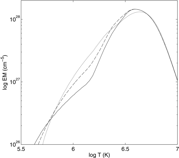
Figure 1. Emission measure as a function of temperature for a loop heated by a single nanoflare. The solid, dashed, and dotted curves show the RL12, EBTEL08, and RTV loss functions. The nanoflare is modeled by a triangular pulse of duration 100 s and peak heating 0.38 erg cm−3 s−1.
Download figure:
Standard image High-resolution imageCargill (1994) noted that below T(EMmax), EM(T) ∼ n2τrad, where τrad ∼ T1−α/n is the instantaneous radiative cooling time. Assuming that T ∼ n2 in the radiative phase (Serio et al. 1991; Jakimiec et al. 1992; Reale et al. 1993; Cargill et al. 1995), the result EM ∼ T3/2−α ∼ T2 arises from a simple fit to the RTV losses. More generally, the radiative phase has T ∼ nl, with l ∼ 1 for very long loops (Bradshaw & Cargill 2010b) and l ∼ 2.5 from short ones (Reale et al. 1993; Bradshaw & Cargill 2010b) and one finds EM ∼ T1/l + 1 − α (Cargill & Klimchuk 2004; Bradshaw et al. 2012). So steeper loss functions (more negative α) give larger values of a, as seen in Figure 1. The largest value of a to be expected from a single nanoflare is of the order of three for the case of a very long loop (L > 1010 cm) and steep loss function. Figures 2 and 3 show both the EBTEL08 and RL12 losses. Figure 4 shows EBTEL08 losses.
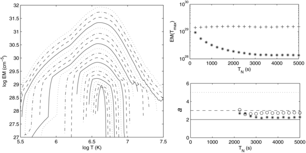
Figure 2. Left panel shows the emission measure as a function of temperature for nanoflare trains with constant energy nanoflares. The 20 curves are associated with different delay times between the nanoflares (TN between 250 and 5000 s). The lowest curve corresponds to TN = 250 s and the highest to TN = 5000 s. Each curve is shifted vertically by 0.2 on a log scale with respect to the previous one as TN increases. The four line styles break TN up into groups of 1000 s. The top right panel shows the maximum value of the emission measure; the upper curve (+) shows the EM integrated over the entire temperature range. The lower right shows the slope of the emission measure below the maximum temperature. The three horizontal lines correspond to a = 2, 3, and 5. Solutions where the EM vanishes at a temperature above 106.25 are not shown so that only the upper 12 curves on the left are represented. Stars and circles are the EBTEL08 and RL12 radiative losses.
Download figure:
Standard image High-resolution image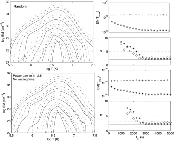
Figure 3. Results for cases with a random distribution of equally space nanoflares (top panels) and for a power law distribution with slope m = −2.5 (lower panels). The formats are the same as Figure 2.
Download figure:
Standard image High-resolution image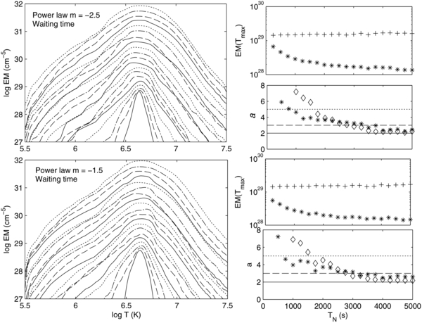
Figure 4. Results for cases with a power law distribution of nanoflares with slope m = −2.5 (top panels) and m = −1.5 (lower panels). In both cases, waiting times between the nanoflares are included so that TN on the horizontal axis is now an average over the nanoflare train. Stars (diamonds) in the lower right panel correspond to nanoflare trains with Q ∝ TN (TN2). The other panels have Q ∝ TN.
Download figure:
Standard image High-resolution image3.1. Equally Separated Nanoflares
Both physical expectations and the results of Warren et al. (2011) suggest that the separation between individual nanoflares (TN) is the key parameter in understanding EM(T). The left panel of Figure 2 shows EM(T) for a set of 20 nanoflare trains, each running for 80,000 s, with 2L = 80 Mm and Hn = 8.3 × 10⁻³ erg cm−3 s−1 (similar parameters to those of Warren et al. 2011). Within each train, the nanoflares have the same energy, and the time between each is identical. Each curve shows a different value of TN, which increases from 250 to 5000 s in increments of 250 s. These values of TN give H0 = 0.03–0.44 erg cm−3 s−1 as one moves from HF to LF regimes. The sharply peaked curves have small values of TN (HF nanoflares), and the broad distributions have large TN (LF nanoflares). For clarity, as TN increases, each curve is shifted upward by 0.2 on a log scale with respect to the previous curve. The line styles break TN into groups of four: TN = 250, 500, 750, 1000 s, etc.
The peak of the EM (EMmax) occurs at roughly 106.6 K for all cases, in agreement with the AR core studies. For TN ⩾ 3000 s, EM(T) extends to below 1 MK. For smaller TN, there is an increasing range of temperatures below which there is no emission, and for TN = 250 s, EM(T) is very sharply peaked. The following should be noted: (1) the curves are truncated below the point where EM(T) falls to the background corona value and (2) the steep downturn of these truncated curves off the "main sequence" of EM is a consequence of the assumption that T, and hence EM(T), is distributed over a narrow range about its average.
The upper right panel of Figure 2 shows EMmax as a function of TN. As TN decreases, EMmax increases by roughly a factor of five. This reflects the fact that the emission becomes more localized in temperature. The upper curve (+ sign) shows the quantity , where DEM(T) is the EM differential in temperature, as calculated by EBTEL. There is a variation of 15% over all TN. (This quantity has no strict meaning in the language of EM analysis, unless EM(T) is strongly peaked around some value (Δlog10T ± 0.3), but its near-constancy reflects the fact that roughly the same quantity of plasma is radiating in all cases.) While not shown, T(EMmax) shows little dependence on TN.
The lower right panel shows the dependence of a on TN, where EM ∼ Ta below T(EMmax). The three horizontal lines correspond to a = 2, a = 3, and a = 5. These are, respectively, one expected value for LF nanoflares, the maximum possible value for LF nanoflares, and the maximum deduced by the various data-based investigations. The stars and circles are the EBTEL08 and RL12 radiative losses, respectively. The quantity a is calculated between T(EMmax) and a sequence of 12 lower temperatures, increasing from 106 to 106.25 K, and then averaged. If EM at any relevant temperature drops below 10−3 EMmax, the associated value of a is excluded from the averaging. Although this eliminates fluctuations in a, a calculation of a using the lowest physically meaningful value of EM above 1 MK is often also adequate.
The slope of EM(T) changes as one moves away from LF nanoflares, with a of order 2 (2.7) for the EBTEL08 (RL12) losses when TN > 2000 s. For TN less than 2000 s, the values of a are undefined (and so not shown) since there is no plasma for a significant range of temperatures above 106.25 K. The sharp transition in a at TN < 2000 s is due to the loop being reheated before it can cool below 106.25 K. There is a very small intermediate range of TN where a lies above 2 and below 5 but is not evident with a 250 s resolution of TN. Thus, very precise tuning of TN is required to account for the observed range of a. This seems unlikely.
While the behavior of the plasma above T(EMmax) is not central to this paper, it merits comment. There is significant material at these temperatures for LF heating, and EM ∼ T−5 in the vicinity of 10 MK. This is in reasonable agreement with the predicted scaling of T−11/2 (Cargill & Klimchuk 2004) which arises for similar reasons to that in the radiative phase: EM(T) ∼ n2τc ∼ n3/T5/2 where τc ∼ nL2/T5/2 is the conductive cooling time (e.g., Cargill et al. 1995). At constant pressure, as assumed in Cargill & Klimchuk (2004), a p3/T11/2 scaling follows. For our examples, the pressure is not exactly constant during the conductive cooling phase, leading to a weaker scaling. The very extreme temperatures (107.5 K) for the LF runs arise because a heat flux limiter is used in EBTEL (Klimchuk et al. 2008). When only the Spitzer conduction formalism is used, these very high temperatures disappear. In fact, the physics of conductive cooling is complicated at such high temperatures (e.g., West et al. 2008), and a proper theoretical study of high temperature AR plasmas is badly needed.
The upper panels of Figure 3 show results for a random distribution of nanoflare energies with a factor 10 difference between minimum and maximum values of Hn and constant TN in each nanoflare train. Again, 20 nanoflare trains are shown with TN increasing from 250 to 5000 s. For this flat distribution, most of the energy is injected in large events. The results do not change greatly from Figure 2 for large and small values of TN but there is a broadening of EM(T) for intermediate values, giving a between 3 and 10 for both loss functions around TN = 2000 s. However, there is still quite a sharp change from a ∼ 2 to values of TN where a is undefined, roughly 500 s; again, this will require quite precise tuning of TN..
3.2. Power Law Distributions of Nanoflares
We next consider the nanoflare distribution to be a power law, N(Q) ∼ Q−m. It is well known that when the power law extends over several decades, the value m = 2 corresponds to the transition between the input power dominated by large (small) events for m < 2 (m > 2): Hudson (1991). Data from solar flares suggests that m < 2 (Crosby et al. 1993; Crosby 2011). On the other hand, firm evidence for the value of m at nanoflare energies is difficult to obtain. Different analysis methods give values of m > and <2 for observed non-flaring brightenings (Parnell 2004). There is also ambiguity about how N(Q) is modified by plasma cooling processes prior to any observation of intensity fluctuations at EUV wavelengths (Parenti et al. 2006). Further, given that nanoflares may be <1024 erg (see below and Testa et al. 2013), any plasma brightening due to a single nanoflare may be close to unobservable.
Such power law distributions also arise from theoretical and computational modeling of a driven corona (see Charbonneau et al. 2001 for a review). For example, Lu & Hamilton (1991) and Lu et al. (1993) obtained m ∼ 1.4 for a simple model of the coronal field in a self-organized state. Vlahos et al. (1995) used different "rules" governing field dissipation to show that m > 2, at least for smaller events. Numerical simulations of a nanoflare-heated corona (e.g., Rappazzo et al. 2008; Bingert & Peter 2013) also lead to power law distributions generally with m < 2. An important caveat to all these results is that one is unsure whether the correct dissipative processes are modeled and/or resolved. We subsequently consider values of m > and <2 but continue to restrict Q to be distributed over a decade, with the individual nanoflare energies being calculated to ensure the correct total power (8.3 ×10⁻³ erg cm−3 s−1) is going into the sub-loop. The lower panels of Figures 3 show results for m = 2.5 and are quite similar to the random distribution discussed above.
Next, we propose that the time between consecutive nanoflares depends on the energy of the second nanoflare, since larger nanoflares will take longer to build up their energy. Two scalings are considered: Q ∝ TN and Q ∝ TN2, with the motivation discussed fully in Section 4 where we will argue that the former is the more relevant scaling for AR core loops. The results for m = −2.5 (−1.5) are shown in the upper (lower) parts of Figure 4, where the horizontal axes in the right hand column now show an average TN, so that, for example, when 〈TN〉 = 1000 s, the delay between individual nanoflares can range from a few hundred to 3000 s. The left and upper right panels show examples with Q ∝ TN only. The lower right panel, which shows the dependence of a on TN, has stars denoting Q ∝ TN and diamonds Q ∝ TN2.
Instead of the abrupt transition in TN over a few hundred seconds between a being of the order of 2–3 and having no physical value, a now slowly increases from ∼2 for large TN to ∼5 for TN over a few thousand seconds. The transition to sharply peaked EM(T) occurs at larger TN for Q ∝ TN2. The lower panels show a similar result holds for the flatter power law (m = 1.5). It seems possible that the range of a observed could correspond to differences between the various ARs (e.g., magnetic field strengths and small-scale field topologies) leading to different detailed dissipation processes (a range of TN and hence Q) within a generic nanoflare scenario. The important point is that one is no longer tied to a very narrow range of TN to give the observed range of a.
The reason behind this result is seen in Figure 5 which shows the temperature and density evolution for two cases with a power law nanoflare distribution, Q ∝ TN, and m = 2.5, where the upper (lower) rows having equally spaced nanoflares (a "waiting time" between nanoflares). The important point is that when a waiting time is included, the plasma heated by a nanoflare prior to a much larger event cools through the entire temperature range to and below 1 MK, so contributing to EM over a broad temperature range. This does not happen when the nanoflares occur at equal intervals. The slow increase in a as 〈TN〉 decreases is because there are an increasing number of nanoflares and so fewer cases where a long delay occurs prior to a large nanoflare. Eventually, for some small TN, the delay between nanoflares is always short enough that in no cases is there cooling to 1 MK. (Note that the cooling time is relatively independent of the energy in the nanoflare; See the Appendix and Cargill et al. 1995). For Q ∝ TN2, there is a smaller range of times between nanoflares for a given 〈TN〉, so that as 〈TN〉 decreases, the probability decreases of a sub-loop cooling below 1 MK prior to reheating. This is evident in Figure 4, with larger values of a between 1000 and 2000 s.
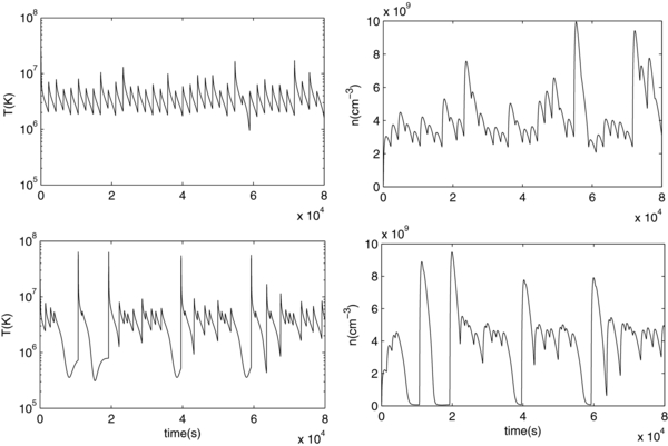
Figure 5. Temperature and density during two runs with a nanoflare power law, slope m = −2.5. In the upper panel, the nanoflares are distributed equally, while in the lower panel, a waiting time proportional to the nanoflare energy is included.
Download figure:
Standard image High-resolution image3.3. Parameter Variations
We now study the effect of changing L and Hn. The important quantity in understanding these results is the ratio of TN to the time taken for the sub-loop to cool to below 1 MK from its peak temperature (the cooling time, τcool: typically in the range 1000–3000 s). In general terms, if τcool < (>) TN, one is in the LF (HF) nanoflare regime. An expression for τcool is derived in the Appendix for the case of a radiative loss function that has a single power law dependence on temperature. It is linearly proportional to L and depends only weakly on the nanoflare energy (see also Cargill 1993; Cargill et al. 1995).
We define the quantity  to be the value of TN below which no valid value of a is obtained (i.e., when τcool > TN). Table 2 summarizes the results for Q ∝ TN. The upper three rows show
  for a constant nanoflare train (as in Figure 2) and when a waiting time between nanoflares is introduced (Figure 4) for three loop lengths. The scaling between
  and L is not precisely linear, as predicted in the Appendix, but is adequate given the approximations made in obtaining Equation (A2); see Cargill et al. (1995) for more details. (For very short loops,
  is <250 s when a waiting time is included.) The last three rows show a as a function of Hn and L for TN
  ; this is independent of the form of the nanoflare train distribution. Here, a lies in a fairly narrow range but does increase as L increases, as we discussed at the start of this section, due to the influence of gravitational stratification in long loops. Further, the net effect of increasing L and/or Hn is to raise the entire range of a over all TN.
Table 2. Summary of Parameter Variations
| 2L (Mm) | 40 | 80 | 120 |
 (s): constant train (s): constant train |
1000 | 2250 | 4500 |
〈 〉(s): waiting time 〉(s): waiting time |
... | 250 | 1000 |
| Hn (10−3 erg cm−3 s−1) | ... | ... | ... |
| 4 | a = 1.7 | 1.9 | 2.5 |
| 8 | a = 2 | 2 | 2.6 |
| 16 | a = 2.2 | 2.2 | 2.6 |
Notes. The second and third rows show the critical time between nanoflares ( ) as a function of loop lengths for a nanoflare train with equally spaced nanoflares and one with waiting time included in a power law distribution. The last three rows and columns show the asymptotic value of a for TN
  as a function of the loop heating rate and loop length for an equally spaced nanoflare train.
Download table as: ASCIITypeset image
4. DISCUSSION
The results of the previous section can be summarized as follows.
- 1.Uniform nanoflare trains lead to a of the order of 2–3 (depending on the radiative loss function used) above some value of TN. Below that value, the EM distribution is sharply peaked around the temperature of peaked emission. Random distributions lead to similar results.
- 2.Power law distributions of nanoflares lead to a broad range of a (2 < a < 5) if there is a waiting time before a nanoflare that depends on its energy. Larger values of a arise for smaller TN.
- 3.The loop length is a key parameter. Long (short) loops have a higher (lower) value of
 and larger (smaller) value of a. The results show little dependence on the magnitude of the energy released in the loop.

Points (1) and (2) suggest that uniform nanoflare trains cannot produce the observed range of EM slopes, and that quite steep power laws are required, though an exception to this occurs when a HF nanoflare train is "tapered" (Reep et al. 2013). It also appears as if the observed values of a require quite small values of TN. This has important implications, as discussed in a moment. Regarding point (3), we note that Warren et al. (2012) find larger a for larger AR areas. From their images, it is clear that there is no direct one-to-one relation between AR area and loop length, though one would suspect that larger ARs would contain longer loops.
We now discuss the implications for nanoflare heating. Defining Bt and Ba as the reconnecting (transverse) and axial (guide) field components in the corona (following Parker 1988), and v a typical photospheric velocity, then the energy supplied to the corona is roughly BtBav/4π erg cm−2 s−1, with Bt ≈ Bavt/2L. If we assume a nanoflare involves the release of all the stored magnetic energy (assumed to be contained in Bt), then  where BtN = Bt(t = TN), the time taken to build up to a nanoflare energy is TN = (2L/v)(BtN/Ba), and Q ∝
  . The nanoflare energy can then be related to Hn (Section 2.3) to give the condition
  that needs to be met to satisfy the coronal energy requirements.1 If we take typical AR numbers, Hn = 8 × 10⁻³, Ba = 150 G, 2L = 8 × 10⁹, v = 1 km s−1, then BtN/Ba ∼ 0.7, TN = 56,000 s and Q is of order 1026 erg for Ah ∼ 1014 cm2 and 1024 erg for Ah ∼ 1012 cm2, with smaller Hn having smaller values of BtN/Ba and TN. Two points should be noted for the values of Hn used in Table 2: (1) the build-up time is a factor 5–20 times longer than the TN required to reproduce the EM(T) results discussed in Section 3 and (2) any model which assumes Bt ≪ Ba (such as those using reduced MHD; Rappazzo et al. 2008; Dahlburg et al. 2012) will have difficulties in accounting for AR heating.
The discrepancy between a simple nanoflare model that implies a long TN and the observed EM(T) results that require a short TN can be partially resolved as follows. Assume that during the nanoflare, Bt relaxes to Bt0 = Bt − dBtN and replenishment of the coronal energy by footpoint motions begins at Bt = Bt0, with dBt = Bavt/2L and dBtN = BavTN/2L. The rate energy is injected is then vAh(Ba(Bt0 + dBt)/4π)which integrates to give, on rewriting in terms of dBtN, Q = 2LAhdBtN(2Bt0 + dBtN)/8π. For Bt0 = 0, we recover the earlier results. For dBtN = Bt0, Q ∝ TN, Q and TN are both smaller by roughly a factor dBtN/Bt0, while there are Bt0/dBtN more nanoflares, ensuring that the total energy requirements are met. If TN is to be reduced to the range of values required for the observed EM(T), we conclude that the nanoflare must be associated with a small decrease in Bt while Bt0 remains large. Setting TN = 1000 s, and retaining the same values of Ba, Bt0, L, and v as before, dBt = 1.9 G, Q = 3 × 1024 erg for Ah = 1014 cm2, and Q = 3 × 10²² for Ah = 1014 cm2. Q ∼ a few 1023 is inferred from AR moss studies using the Hi-C instrument (Testa et al. 2013).
How this can occur in the frameworks of magnetohydrodynamics is unclear at the moment but one suggestion comes from the idea of helicity conservation. Here, a stressed state does not relax to a potential field but that corresponding to a "constant-α force-free field" (Taylor 1974; Heyvaerts & Priest 1984). Were that state to be close to the stressed one, a small release of energy could be the outcome. Further studies are needed.
The relation between Q and TN is important for our results, and an early discussion of its consequences for a range of astrophysical X-ray sources can be found in Rosner & Vaiana (1978). We note that models of a driven corona such as initiated by Lu and Hamilton (e.g., Lu et al. 1993) and flare observations (e.g., Crosby et al. 1998) suggest that there is little if any connection between Q and TN. However, the waiting times in these cases are evaluated over a large volume (e.g., an entire AR or computational box; see also Charbonneau et al. 2001) and so yield no useful information about TN in a sub-loop such as we are concerned with. Other theoretical models suggest various scalings for "local" waiting times (e.g., Berger 1994; Craig 2001; Wheatland & Craig 2003). Berger (1994) and Sturrock & Uchida (1981) argue that rotational twisting gives Q ∼ TD while Wheatland & Craig (2003) discuss magnetic flux pile-up at a separator leading to Q ∼ TD2. However, none of these examples consider the consequences of injecting energy into a loop that already has a quite stressed field.
5. CONCLUSIONS
We have studied the expected EM distribution as a function of temperature for models of nanoflare heating of AR loop cores, with emphasis on the temporal distribution of nanoflares. The two main results are (1) the best option for obtaining agreement with observed values of the slope of the nanoflare distribution EM(T) ∼ Ta lies in the incorporation of a waiting time prior to a nanoflare that is proportional to its energy and (2) the time separating nanoflares has to be of the order of a few hundred to somewhat over 2000 s, thus ruling out the possibility that a nanoflare involves the relaxation of the coronal field to a near-potential state. We thus argue that nanoflares occur in a corona that is continually stressed, with a small energy release permitting a subsequent rapid replenishment of energy.
Our work has focused solely on slow photospheric driving. However, other authors (van Ballegooijen et al. 2011; Asgari-Targhi & van Ballegooijen 2012; Asgari-Targhi et al. 2013) have developed "turbulent" models that also involve very bursty energy release that one could term nanoflares. In this work, Alfvén waves are injected into the chromosphere and corona by photospheric footpoint motions of the order of 1 km s−1, with a correlation time of the order of a minute. Both footpoints are set in motion and the interaction of counter-propagating waves leads to a rapid turbulent cascade. Although the reduced MHD assumption is made, these models do not suffer from the "energy deficiency" problem discussed in Section 4 (see Table 2 of Asgari-Targhi & van Ballegooijen 2012).
Space does not permit a full discussion of their results but Figure 7 of Asgari-Targhi & van Ballegooijen (2012) is a reasonable sample and shows that for loop lengths of the order 100 Mm, a maximum temperature of the order of 2–3 MK is obtained, consistent with AR observations. In all cases, there is evidence for intermittent energy release, with bursts being separated by a hundred seconds or so, leading to small temperature fluctuations around a constant value (see Figure 9 of Asgari-Targhi & van Ballegooijen 2012). This suggests that such a turbulent heating model cannot account for the observed EM slopes, instead giving a very sharply peaked EM(T). However, with improved numerical resolution, finer spatial structure may appear, perhaps leading to the dissipation occurring in smaller regions.
The Hinode data described earlier in this paper thus appear to impose important constraints on how nanoflare heating may be operating, and it is in a different way from commonly supposed. Indeed, one can finally say that quantitative analysis of coronal heating is at last possible. The other result from this work, and that of Testa & Reale (2012) and Testa et al. (2011), concerns the presence of hot coronal components with temperatures in excess of T(EMmax). This has long been a prediction of nanoflare models (e.g., Cargill 1994, 1995) but is very difficult to interpret due to ionization nonequilibrium (Bradshaw & Cargill 2006), the predicted small EMs, and plasma physics issues associated with heat conduction in very hot plasmas (West et al. 2008). This would appear to be a productive area to focus on following the insights obtained at lower temperatures, as described here.
This work was performed as a contribution to a team supported by the International Space Science Institute (ISSI) and led by Helen Mason and Steve Bradshaw. I am grateful to Harry Warren, Jim Klimchuk, and Steve Bradshaw for helpful discussions and to Aad van Ballegooijen for providing additional information about his work. The referee raised an important issue that led to an improved paper.
APPENDIX: GENERALIZED COOLING TIME
Cargill et al. (1995) evaluated the time taken for a loop to cool from an initial temperature T0 and n0. The analysis assumed that the loop cooled first by conduction and then by radiation, the change between cooling processes occurring at a temperature T*. Analytic solutions due to Antiochos & Sturrock (1978) were used for the conductive phase and the scaling T ∼ n2 (Serio et al. 1991; Reale et al. 1993; Cargill et al. 1995) was used in the radiative phase. As presented in Cargill et al. (1995), the solution was "hard wired" to a radiative loss function RL = χTα = 6 × 10⁻²⁰ T−1/2. We have discussed earlier that recent work has led to greatly increased losses below a few MK, so that in any single function fit, the value of α will be more negative, with χ being adjusted accordingly to give a larger loss at 1 MK. By following the same analysis as Cargill et al. (1995), it can be shown that the total cooling time is

where τc0 and τr0 are the cooling times defined at t = 0:  , τr0 = 3kT1 − α/χn, and τr0 ≫ τc0. One can tidy up Equation (A1) in terms of the loop length and initial pressure (p0):
Setting α = −1/2 recovers the scalings in Equation (14E) of Cargill et al. (1995). If we now relate the initial loop pressure to the energy in a nanoflare using Q = 3n0kT0H0τHLAh/2, Equation (A2) can be used to show that τcool ∼ LQ−(3 + 2α)/(11 − 2α), so τcool scales exactly linearly with L, independent of the loss function slope, and depending weakly on Q.
Footnotes
- 1
The analysis here follows Parker (1988) and differs slightly from that in Lopez-Fuentes & Klimchuk (2010), which in some ways is more complete. We assume the nanoflare arises when one magnetic strand (or sub-loop) is moved with respect to another, whose magnetic field retains Bt = 0. Lopez-Fuentes & Klimchuk assume that both strands acquire a component Bt. This leads to differences of factors of two in some derived quantities but has no influence on the physical conclusions.