


ABSTRACT
We report matched resolution imaging spectroscopy of the CO 3–2 line (with the IRAM Plateau de Bure millimeter interferometer) and of the Hα line (with LUCI at the Large Binocular Telescope) in the massive z = 1.53 main-sequence galaxy EGS 13011166, as part of the "Plateau de Bure high-z, blue-sequence survey" (PHIBSS: Tacconi et al.). We combine these data with Hubble Space Telescope V–I–J–H-band maps to derive spatially resolved distributions of stellar surface density, star formation rate, molecular gas surface density, optical extinction, and gas kinematics. The spatial distribution and kinematics of the ionized and molecular gas are remarkably similar and are well modeled by a turbulent, globally Toomre unstable, rotating disk. The stellar surface density distribution is smoother than the clumpy rest-frame UV/optical light distribution and peaks in an obscured, star-forming massive bulge near the dynamical center. The molecular gas surface density and the effective optical screen extinction track each other and are well modeled by a "mixed" extinction model. The inferred slope of the spatially resolved molecular gas to star formation rate relation, N = dlogΣstar form/dlogΣmol gas, depends strongly on the adopted extinction model, and can vary from 0.8 to 1.7. For the preferred mixed dust–gas model, we find N = 1.14 ± 0.1.
Export citation and abstract BibTeX RIS
1. INTRODUCTION
In our Milky Way (MW) and nearby external galaxies, stars form in dense, molecular gas clouds (e.g., McKee & Ostriker 2007). In massive disk galaxies averaged over scales of several kiloparsecs or more, the surface densities of cold gas and star formation are empirically well correlated through a simple power-law relation, the "Kennicutt–Schmidt" (KS) relation (Schmidt 1959; Kennicutt 1998a, K98; Kennicutt & Evans 2012),

where N = 1.4 (±0.15) if Σgas = ΣHI+H2 (Kennicutt 1998a, 1998b, 2007), above a threshold of ∼10 M☉ pc−2. Here the brackets denote averages over the galaxy, beam, or region considered. A simple physical motivation for Equation (1) comes from considering the star formation rate per volume and making the plausible Ansatz for the volumetric gas to star formation rate relation
where  are the star formation rate per volume, the gas density, and the free fall timescale in that volume, and εffis the star formation efficiency per free fall timescale (εff ∼ 0.02; K98; Kennicutt & Evans 2012; Krumholz & Tan 2007; Krumholz et al. 2012). For a constant gas/star formation scale height hz, Equation (1) follows then from Equation (2), with
  .
.
From spatially resolved mapping of molecular gas (as traced in the CO 2–1 line in the IRAM HERACLES survey), along with HI (from the VLA THINGS survey) and star formation (from Galex FUV + Spitzer 24 μm continua, or Hα + 24 μm continuum) in ∼30 nearby disk galaxies, Bigiel et al. (2008, 2011), Leroy et al. (2008, 2013), and Schruba et al. (2011) have found that the star formation surface density is correlated most strongly with the molecular column density, rather than with the sum of atomic and molecular column densities. These authors find that the "molecular" KS relation simplifies to a linear relation (N = 1 ± 0.15), such that Equation (1) becomes 〈Σstar form〉 = 〈Σmol gas/τdepl〉, or SFR = Mmol gas/τdepl, with a molecular gas depletion time18 of ∼1–2 Gyr (see also Rahman et al. 2012). The residual scatter of the KS relation is ±0.3 dex (K98; Bigiel et al. 2008).
Saintonge et al. (2011a, 2011b, 2012) have measured the molecular gas content from galaxy-integrated CO 1–0 observations in a purely stellar mass selected sample drawn from SDSS (log M* > 10; all masses in this paper are in units of M☉), including both blue- and red-sequence galaxies. Saintonge et al. confirm the ∼1.5 Gyr depletion timescale for massive disks on the blue sequence of star-forming galaxies (henceforth "main sequence" (MS): Schiminovich et al. 2007; Noeske et al. 2007; Daddi et al. 2007). From these galaxy-integrated data, Saintonge et al. (2012) find a global molecular KS relation of slope N = 1.18 (±0.24). They observe structure within the scatter around this relation, with galaxies having low (high) stellar mass surface densities lying systematically above (below) the mean relation, suggesting that ΣH2 is not the only parameter controlling the global star formation in galaxies. On scales less than a few hundred parsecs, the KS relation breaks down in spatially resolved observations in the MW (Murray 2011) and in external galaxies (Onodera et al. 2010; Schruba et al. 2010; Liu et al. 2011; Calzetti et al. 2012), presumably because of evolutionary effects.
Recently it has become possible to carry out the first systematic studies of the molecular gas content and the molecular KS relation in massive z > 1 star-forming galaxies, near or slightly above the MS (henceforth called SFGs or MS SFGs; Tacconi et al. 2010; Daddi et al. 2010a, 2010b; Genzel et al. 2010). In the PHIBSS survey, Tacconi et al. (2013) find N = 1.05 ± 0.17 from galaxy-integrated measurements in 50 z = 1–1.5 MS SFGs and deduce an average depletion timescale of 0.7 ± 0.1 Gyr.
The next step is to explore whether a near-linear high-z KS relation also applies on sub-galactic scales. In the present paper, we report an analysis of the distribution of molecular gas, extinction, stars, and star formation rate in a very massive z ∼ 1.5 MS SFG within the PHIBSS sample, for which we have assembled, for the first time, all the information to carry out a spatially resolved analysis of the z > 1 KS relation.
Throughout the paper, we use the standard Wilkinson Microwave Anisotropy Probe ΛCDM cosmology (Komatsu et al. 2011) and a Chabrier (2003) initial stellar mass function.
2. OBSERVATIONS
2.1. The "Plateau de Bure High-z Blue-sequence Survey" (PHIBSS)
The PHIBSS survey (Tacconi et al. 2010, 2013) explores the cold molecular gas from 12CO 3–2 line emission in massive (log M* > 10.4) MS SFGs at z = 1–3. The targets have been selected from parent samples found in large UV/optical/IR look-back imaging surveys, mainly in the AEGIS (DEEP2/DEEP3: Davis et al. 2007; Cooper et al. 2012), GOODS-N (Daddi et al. 2010a; Magnelli et al. 2012) and Caltech QSO fields (Steidel et al. 2004; Erb et al. 2006). With stellar mass and star formation rate cuts of log M* > 10.4 and SFR ⩾ 30 M☉ yr−1, PHIBSS provides a fair census of the massive tail of the star-forming population in the stellar-mass–star-formation-rate plane along the MS line and upward, at the peak epoch of cosmic star formation. The MS population accounts for ⩾90% of the cosmic star formation rate at z ∼ 1–2.5, and as such samples "normal" massive star-forming galaxies near equilibrium growth, rather than rare major merger-induced starbursts (Noeske et al. 2007; Daddi et al. 2007; Reddy et al. 2005; Rodighiero et al. 2011; Elbaz et al. 2011; Nordon et al. 2012).
2.1.1. EGS 13011166
EGS 13011166 (z = 1.53, log M* = 11.1) is located in the massive tail of the z ∼ 1–2 MS SFGs, and about 0.2 dex above its center line (left panel of Figure 1). On the Advanced Camera for Surveys (ACS) and WFC3 V–H images of the AEGIS survey field, the galaxy is characterized by a very clumpy and amorphous rest-frame UV- and optical light distribution, with a dozen kiloparsec-scale bright clumps distributed over ∼5'' (∼40 kpc, right panel of Figure 1). Table 1 gives a summary of the salient parameters of the galaxy.
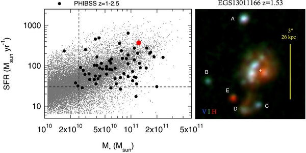
Figure 1. Left: the location of EGS 13011166 in the stellar-mass–star formation rate plane (filled red circle), compared to the overall PHIBSS CO 3–2 survey of z ∼ 1–3 SFGs (filled black circles; Tacconi et al. 2013), and the underlying MS of z ∼ 1.5–2.5 SFG population as derived in the COSMOS field with the BzK color–magnitude criterion (gray dots; McCracken et al. 2010; Mancini et al. 2011). Right: V (blue) – I (green) – H (red)—three band HST image of EGS 13011166, all on a sqrt(F) color scale. The images were smoothed to ∼0 25 FWHM. A–E denote prominent star formation clumps. The small white cross marks the position of the stellar and star formation rate surface density peaks (Figure 2).
Download figure:
Standard image High-resolution imageTable 1. Properties of EGS 13011166
| Coordinates | R.A. = 14h19m45 15 decl. = 52052'276 15 decl. = 52052'276 |
|---|---|
| Redshift | 1.53068(5) |
| R1/2 (kpc) (8.62 kpc arcsec−1) | 6.3 ± 1 (UV/optical), 6.3 ± 1 (CO) |
| b/a, i | 0.5 (+0.15, −0.1), 60 ± 150 |
| nSersic | 1 ± 0.5 |
| vrot, vc (km s−1) | 307 ± 50, 320 ± 54 at peak |
| σ0, vrot/σ0 | 52 ± 10, 6.1 ± 2 |
| F(Hα) (10−16 erg s−1 cm−2) | 4.5 ± 1 |
| Fco 3–2 (Jy km s−1) | 2.1 ± 0.2 |
| F[nii] 6585/FHα, F[sii] 6718/FHα | 0.37 ± 0.01, 0.25 ± 0.04 |
| 12 + log{O/H}PP04, log U | 8.65, −3.5 ± 0.3 |
| 12 + log{O/H}D02 | 8.77 |
| M*, Mmol gas, Mdyn (1011 M☉) | 1.2 ± 0.4, 2.6(±0.8)×α4.36, 3.0 (±0.6) × (0.81/sin(i))2 |
| SFRUV, SFRSED 0, SFRFIR | 23 ± 7, 150 ± 30, 352 ± 80 |
| SFRHα 0, SFRHα 00 (M☉ yr−1) | 114 ± 25, 560 ± 130 |
| SFRtot = SFRUV + SFRFIR | 375 ± 80 |
| 〈Σmol gas〉 (M☉ pc−2), 〈QToomre〉 | 103, 0.45 ± 0.25 |
| 〈Σstar form〉 (M☉ yr−1 kpc−2) | 1.5 |
| τdepl = Mmol gas/SFRtot (Gyr) | 0.7 (galaxy integrated) |
| ηout = dMout/dt/SFRHα 00 | 1.5 (±1) × (vout/600 km s−1) × (R1/2/6.3 kpc)−1 × (ne/50 cm−3)−1 |
Download table as: ASCIITypeset image
We selected EGS 13011166 for high-resolution follow-up imaging spectroscopy in CO 3–2 and Hα, for the following reasons.
- 1.The large star formation rate and large extent made subarcsecond resolution CO observations with the A-configuration of the PdBI feasible;
- 2.The source is at a redshift (z = 1.53) where Hα, redshifted into the H band, is relatively unaffected by strong OH night-sky emission lines;
- 3.
- 4.The clumpy UV/optical appearance of EGS 13011166 is quite typical for many other z ∼ 1.5–2.5 SFGs, and we wanted to test whether the gas kinematics is more regular, and whether these clumps are also visible in molecular emission.
2.2. IRAM PdBI CO Observations and Data Analysis
EGS 13011166 was observed for 31 hr in the Winter 2012 in the A, B, and C configurations of the 6 × 15 m IRAM Plateau de Bure Millimeter Interferometer (Guilloteau et al. 1992; Cox et al. 2011). We observed the 12CO 3–2 rotational transition (rest frequency 345.998 GHz), which is shifted into the 2 mm band. The observations take advantage of the new generation dual polarization receivers that deliver receiver temperatures of ∼50 K single side band (Cox et al. 2011). Depending on the tapering and configurations used, the synthesized beam had an FWHM between 07 × 085 (for natural weighting in the most sensitive combination A+B+C, rms per channel 0.25 mJy) and 056 × 068 (in A+B).
System temperatures ranged between 100 and 200 K. Every 20 minutes we alternated source observations with a bright quasar calibrator within 15° of the source. The absolute flux scale was calibrated on MWC349 (S3 mm = 1.2 Jy). The spectral correlator was configured to cover 1 GHz per polarization. The data were calibrated using the CLIC package of the IRAM GILDAS software system and further analyzed and mapped in the MAPPING environment of GILDAS. Final maps were cleaned with the CLARK version of CLEAN implemented in GILDAS. The absolute flux scale is better than ±20%. The spectra were analyzed with the CLASS package within GILDAS.
To convert the measured CO 3–2 fluxes to molecular gas masses (including a 36% upward correction for the presence of helium), we used an MW conversion factor (α = 4.36 M☉ (K km s−1 pc2)−1; see footnote 18) and adopted a Rayleigh–Jeans brightness temperature ratio of the 1–0 to the 3–2 line of 2 (see Tacconi et al. 2013 for details).
The astrometry of the PdBI maps is accurate to ±02, which is consistent with the good spatial alignment of the CO map and the extinction map inferred from the HST imagery and discussed in Section 3.1.
2.3. LUCI@LBT Hα Observations and Data Analysis
We obtained optical spectroscopy data of EGS 13011166 with LUCI (Ageorges et al. 2010; Seifert et al. 2010; Buschkamp et al. 2010) mounted at the Gregorian focus of the 2 × 8.4 m Large Binocular Telescope (LBT) on Mount Graham in Arizona (Hill et al. 2006). LUCI is an NIR camera and spectrograph that allows multi-object spectroscopy at spectral resolving powers of R ∼ 3900 over a 2 5 × 4' field using user-defined masks.
The data were taken over six consecutive nights in 2012 March. We obtained spectra through a 4'× 075 wide slit oriented north–south (cut in a mask), with 025 pixels along the slit. We scanned the galaxy in the east–west direction to obtain spatially resolved spectra both along and perpendicular to the slit. We used nine steps of half the slit width (i.e., 0375) to obtain Nyquist sampling over an extent of 34. The acquisition was done by centering the slit on a star 80'' away from the galaxy. In contrast to integral field spectroscopy, where the spectra at all spatial elements are obtained simultaneously, the slit scanning technique obtains spectra at different positions asynchronously and therefore possibly under different atmospheric circumstances. For that reason, we did not stare at one position before moving to the next, but cycled, typically, through five different slit positions in one night. In addition, an offset of 10'' along the slit was applied between each five-minute exposure, following an ABAB pattern. As the seeing was rather stable during the observing run, the point-source functions (PSFs) obtained in each slit are similar. After each night, we evaluated the signal-to-noise obtained and decided which positions needed more exposure. This led to inhomogeneous exposure times over the field of view, but improved the signal-to-noise obtained in the outskirts of the galaxy. We nevertheless always obtained exposures of the (central) position centered on the acquisition star to monitor its PSF and position on the detector. The number of exposures per slit position varied from 5 to 33, amounting to a total exposure time of 15 hr. The observations were reduced with the pipeline developed at MPE for LUCI (J. Kurk et al., in preparation). The pipeline includes removal of bad pixels and persistence effects, cosmic ray masking, wavelength calibration employing OH sky lines, rectification and linearization, background subtraction, and co-addition of the exposures. We flux calibrated on an A0V star. We did not attempt to correct for (differential) slit losses. The nine reduced slit positions were co-registered to obtain data and associated noise cubes of the galaxy and the star. The latter has an FWHM of 07 along and 08 across the slit direction. The spectral resolving power achieved near the Hα line at λ = 1.6610 μm is R ∼ 3900 FWHM, as measured from nearby OH lines.
The a priori absolute astrometry of the LUCI data is probably no better than ±07. However, by extracting a continuum H-band map from the H-band cube, we were able to co-align the Hα map on the HST H-band image, to an accuracy of ±035.
2.4. HST Maps of Stellar Mass Surface Density, Star Formation Rate, and Extinction
We derived resolved high-resolution HST maps of the effective V-band screen extinction, and of the extinction corrected stellar mass and star formation rate surface density distributions within EGS 13011166, following the procedures outlined by Förster Schreiber et al. (2011) and Wuyts et al. (2011a, 2012). Briefly, the available multi-wavelength HST imaging was matched to the resolution of the F160W image (018 FWHM), employing the PSFMATCH algorithm in IRAF. A Voronoi 2D binning scheme (Cappellari & Copin 2003) was applied in order to achieve a minimum signal-to-noise level of 10 per spatial bin in the F160W band. Subsequently, we fitted Bruzual & Charlot (2003) stellar population synthesis models to the photometry of each spatial bin, adopting assumptions that are standard in the literature. We allowed ages since the onset of star formation between 50 Myr and the age of the universe, and visual extinctions in the range 0 < AV < 4 with the reddening following a Calzetti et al. (2000) recipe. We assume the metallicity of the stellar population is solar across the galaxy (see Section 3.1.3) and allow exponentially declining star formation histories with e-folding times down to τ = 300 Myr. In addition, we also explored delayed tau models (SFR ∼ t * exp(−t/τ)), which at early times (t < τ) feature rising star formation rate levels, and find similar results. For comparison to the other data discussed in this paper, the HST images were smoothed with a Gaussian kernel of the desired final FWHM.
3. RESULTS
The data presented in this paper allow, for the first time, a spatially resolved comparison of the distribution and kinematics of the molecular and ionized gas (FWHM resolution ∼6 kpc), as well as the distribution of the star formation rate, extinction, and stellar surface density (FWHM resolution ∼1.6–2.5 kpc), in a luminous active MS SFG at the peak of the galaxy formation epoch. We begin with a qualitative comparison of the individual tracers, followed by a quantitative comparison of the kinematics, the extinction/molecular gas maps, and the star formation rate/molecular gas maps (see Table 1 for a summary of the basic inferred parameters).
3.1. Comparison of the Different Tracers
3.1.1. Rest-frame UV/Optical Continuum Maps
The clumpy and irregular rest-frame UV/optical light distribution of EGS 13011166 (right panel in Figure 1) is similar to many other z > 1 SFGs (Cowie et al. 1996; Giavalisco et al. 1996; van den Bergh et al. 1996; Elmegreen et al. 2005, 2007; Elmegreen & Elmegreen 2006; Förster Schreiber et al. 2009, 2011; Law et al. 2012; Wuyts et al. 2012). The main body of the galaxy is fitted by an nS = 1 ± 0.5 Sersic profile in the I/J/H light profiles, with an effective radius R1/2 = 6.3 ± 1 kpc and inclination 60° ± 15°. In addition, there are five additional prominent clumps outside that main body and distributed over ∼40 kpc (labeled A through E in the right panel of Figure 1).
There is an east–west color gradient, with the eastern half of the central galaxy much bluer than the western half, perpendicular to the major axis of the galaxy (P.A. −36° west of north). This color gradient is largely due to extinction being much higher in a ridge on the western side, as demonstrated in the extinction map derived from the spectral energy distribution (SED) fitting to the HST imaging photometry (bottom right panel in Figure 2). The western half of the main galaxy might be in front, such that there is a large column of dust toward the central regions along that line of sight. The centroids of the stellar density and star formation rate are embedded in and slightly east of this dust extinction lane (center and right panels in the top row, as well bottom right panel of Figure 2).

Figure 2. Comparison of images. Top row: integrated CO flux map in color (ABC-configurations, 07 × 08 FWHM) and (left) WFC3 HST H-band map as white contours, ∼03 FWHM; (center) inferred stellar mass distribution from SED fitting white contours, 075 FWHM; and (right) extinction-corrected star formation rate distribution inferred from SED fitting (white contours, 075 resolution). Bottom row: (left) CO-integrated flux map in white contours (AB-configuration, 056 × 068 FWHM) and HST WFC3 H-band map (red, 03 FWHM) and ACS V-band map (green, 03 FWHM), (center) CO-integrated flux map in white contours, (AB-configuration, 056 × 068 FWHM) and HST AV-map (red, 035 FWHM) and (right) ACS V-band map (blue, 035 FWHM). (Right) HST ACS V-band (green), and AV-map in white contours and stellar mass map (red), both inferred from SED modeling. All HST maps are smoothed to 035 FWHM. The pixel scale is 006.
Download figure:
Standard image High-resolution imageThe stellar surface density distribution inferred from the SED fitting is much smoother than the V–H light distributions, consistent with the clumpy distribution of dust, and similar to many other z ∼ 1–2.5 SFGs (Wuyts et al. 2012). EGS 13011166 thus fits in with the general result of Wuyts et al. (2012) that the rest-frame UV clumps are mostly sites of low-extinction star formation.
3.1.2. CO
The molecular surface density map inferred from the CO flux map correlates quite well with the inferred AV-map (bottom central panel of Figure 2), and also with the stellar density (top central panel) and extinction corrected star formation rate (top right panel) maps. However, the brightest CO peak is ∼05 southeast of the kinematic center (see below) and the stellar and star formation maxima inferred from the extinction corrected UV/optical data. It is unclear whether all or part of this shift is due to a real asymmetry of the molecular gas relative to the extinction distribution, whether it is due to incorrect astrometric alignment, or whether the intrinsic UV/optical emission toward the CO maximum is totally blocked by very large extinction. As we will discuss below, the total dust columns connected to the CO peak correspond to AV ∼ 50; unless this dust is distributed in a clumpy arrangement, any underlying UV/optical emission could in principle be completely blocked. Again, the brightest V-/I-band clumps appear to be mostly east (and one west) of this clumpy ridge of molecular column density.
The strong impact of clumpy extinction and dense clouds on the sub-galactic UV/optical light distribution is not surprising given the large gas and dust columns. Similar effects are also seen in z ∼ 0 starbursts (e.g., Sams et al. 1994; Satyapal et al. 1997).
3.1.3. Optical Emission Line Ratios
Figure 3 summarizes the properties of the strong optical emission lines in EGS 13011166, as extracted from the LUCI data set. The integrated Hα map (upper right) correlates well with the I/V-band stellar light distributions, but peaks near the prominent CO maximum, southeast of the H-band, stellar surface density maxima, and the kinematic center. In contrast, the [N ii]6585 brightness distribution is more compact and peaks very close to the stellar peak (middle right), such that the [N ii]/Hα ratio drops somewhat from 0.45 ± 0.05 near the center to 0.3 ± 0.1 to 1'' off-center, along the major axis of the disk. The galaxy-integrated [N ii]/Hα flux ratio of 0.37 ± 0.01 corresponds to a near solar oxygen abundance, 12 + log{O/H} = 8.65 on the Pettini & Pagel (2004) scale, and 8.77 on the Denicoló et al. (2002) scale.
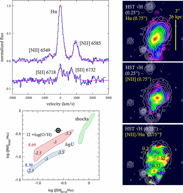
Figure 3. LUCI spectroscopy. Top left: integrated spectrum of EGS 13011166, after removing pixel-by-pixel velocity shifts due to the large-scale rotation. It shows Hα, [N ii] and [S ii] emission lines (blue). The line profile cannot be fit by a single Gaussian. The pink curve is the best fit, double Gaussian profile for all five lines: a "narrow" component of ΔvFWHM = 293(±11) km s−1, and flux ratios [N ii]6585/Hα = 0.37 ± 0.01, [S ii]6718/Hα = 0.25 ± 0.04 and [S ii]6718/[S ii]6732 ∼ 1.3(+0.8, −0.1), and a "broad" component with ΔvFWHM = 680 (±80) km s−1 and flux ratio (Fbroad/Fnarrow)(Hα) = 0.48(±0.13). The broad component is also present in the [N ii] and [S ii] lines. Bottom left: location of ESG13011166 in the [N ii]/Hα and [S ii]/Hα-plane (adapted from Newman et al. 2012b), along with photo-ionization and shock models. The spatially integrated value for EGS 13011166 (large black circle) is well fit with solar metallicity photoionization models with ionization parameter log U ∼ −3.2. Right: overlays the HST H-band map (white contours) on the integrated Hα flux map (top), integrated [N ii]6585 flux map (middle), and [N ii]6585/Hα flux ratio map (bottom).
Download figure:
Standard image High-resolution imageThe combined galaxy-integrated values for [N ii]/Hα and [S ii]/Hα can be well accounted for by photo-ionization of slightly super-solar metallicity gas with a modest ionization parameter of log U ∼ −3.2 ± 0.2 (bottom left panel; Newman et al. 2012b). This value is broadly consistent with the "homogeneous" ionization parameter log U < log(QLyc/(4π R1/22nec)) ∼ −3.5 −log n100 for the flux of Lyman continuum photons of QLyc ∼ 8 × 1043 s−1 from the extinction corrected Hα luminosity, LLyc = 16 LHα and R1/2 = 6.3 kpc, and for an electron density in units of 100 cm−3.
The [N ii]/Hα gradient could then be caused by a shallow abundance gradient, with 12 + log{O/H} ∼ 8.55 in the outer disk and 8.73 in the nucleus (−0.02 dex kpc−1). Given the relatively low resolution of the LUCI data, this value is likely an upper limit and the intrinsic gradient could be steeper. Alternatively, the maximum of [N ii]/Hα at the stellar surface density peak could be due to an active galactic nucleus (AGN) there. While the nuclear [N ii]/Hα ratio can be well explained by photoionization of solar metallicity gas (see above), we cannot exclude that this is strongly affected by beam smearing and that at high resolution the nuclear [N ii]/Hα value may exceed the stellar "photoionization limit" of ∼0.55. There is, however, no X-ray point source associated with EGS 13011166 in the Chandra X-ray catalog of AEGIS (http://astro.ic.ac.uk/content/aegis-x, PI: K. Nandra).
3.1.4. Optical Emission Line Profiles
The upper left panel of Figure 3 shows the galaxy-integrated Hα, [N ii], and [S ii] spectra. The line profile between Hα and the two [N ii] lines does not dip to the zero level, and there are non-Gaussian wings blue- and redward of the two [N ii] lines. The observed spectral profiles either require a non-Gaussian shape or a second, underlying broad emission component (see discussions in Shapiro et al. 2009; Genzel et al. 2011; Newman et al. 2012a). A global two-Gaussian fit to all five emission lines indicates that the broad emission is present in Hα and the [N ii] lines, and perhaps also in the [S ii] lines.
The broad emission could have several causes. It could be due to a galactic ionized gas outflow, as seen commonly in z > 1 MS SFGs (Shapiro et al. 2009; Genzel et al. 2011; Newman et al. 2012a). The broad emission could also be due to high-velocity gas driven by a central AGN. However, the broad emission in EGS 13011166 is present in the forbidden lines as well, thus disfavoring a dense and compact AGN broad line region. Finally, given the relatively poor angular resolution of our Hα data, at least some of the broad wings may due to unresolved, and beam smeared orbital motion near the nucleus, which was not removed by our pixel-by-pixel velocity deshifting method.
In the galactic wind explanation, the width of the broad emission component, ΔvFWHM ∼ 700 km s−1, suggests an average outflow velocity of vout ∼ 600 km s−1 (Genzel et al. 2011), which is comparable to spatially resolved ionized outflows most likely driven by star formation activity ("star formation feedback") seen in many other z ∼ 1–2.5 SFGs (Newman et al. 2012a). AGN-driven winds result in yet broader emission (ΔvFWHM ∼ 1400 km s−1); such winds are detected toward the nuclei of a number of log M* > 11 SFGs (N. M. Förster Schreiber et al. 2013, in preparation). The spatial resolution of the seeing limited LUCI data is not sufficient to distinguish between these two possibilities but the line width is more suggestive of "star formation" feedback.
From the measured line width and broad to narrow flux ratio Fbroad/Fnarrow = 0.48 ± 0.13, a mass outflow rate can be estimated ( ; Genzel et al. 2011). We assume a source radius R comparable to the half-light radius of the galactic disk, and an electron density of ne ∼ 50 cm−3 (Newman et al. 2012a), motivated by the fact the broad [S ii]6718/[S ii]6732 ratio is close to the low-density limit. We infer a mass outflow rate of
  , and a mass loading factor
  = 1.5 ± 1. While obviously quite uncertain, the inferred mass loading parameter is in good agreement with the results of Newman et al. (2012a), who find that z ∼ 1.5–2.5 SFGs exhibit powerful winds with η ∼ 2 above a star formation rate surface density threshold of ∼1.5 M☉ yr−1 kpc−2. The star formation rate surface density of EGS 13011166 is 〈Σstar form〉 = 0.5 × SFR/(πR1/22) ∼ 1.5 M☉ yr−1 kpc−2.
3.2. Gas Kinematics and Modeling
The main body of the galaxy exhibits a regular velocity field in CO (Figure 4) and Hα (Figure 6), with a progression from blueshifted emission (−215 km s−1) in the southeast to redshifted emission (+210 km s−1, both relative to z = 1.5307), along the main body of the galaxy. At our nominal registration, the kinematic centroid and the peak of beam-smeared velocity dispersion are ∼04 ESE of the extinction-corrected stellar and star formation rate peaks. This offset is marginally significant, given the combined relative astrometric uncertainties. The iso-velocity contours in the middle left map of Figure 4 exhibit the characteristic "spider" shape of a rotating disk. The overall velocity and velocity dispersion fields in CO (and Hα; Figure 6) are well fitted by a rotating disk with an exponential half-light radius comparable to that of the UV/optical light distribution (R1/2(CO) = 6.3 ± 1 kpc). The inclination corrected, maximum rotation velocity is 307 ± 50 km s−1.
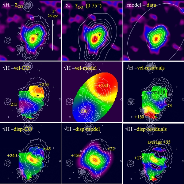
Figure 4. Molecular gas derived kinematics and disk models in EGS 13011166 (all from ABC-configuration data at 07 × 08 FWHM resolution). Top row: CO-integrated flux map in color with white contour maps (from left to right) and the 03 FWHM HST WFC3, stellar mass (as inferred from SED fitting, 075 FWHM) and mass distribution of the best exponential fit model. The middle row shows the CO velocity map (left), the model velocity map (center), and the data minus model residual map, with superpose white contours of the 03 FWHM HST WFC3 map. The bottom row shows the same overlays for the dispersion maps. The black cross denotes the position of the H-band peak that is ∼04(±01) ESE of the stellar mass and star formation rate peaks. Numbers in the individual panels give minimum and maximum values of the color maps, as well as rms and average values of velocity residuals and velocity dispersion residuals.
Download figure:
Standard image High-resolution imageAfter removal of the rotation and instrumental broadening, the average residual dispersion in the outer parts of the galaxy (where the contribution from the residual beam-smeared rotation is smallest) is σ0 = 52 ± 10 km s−1. The resulting ratio vrot/σ0 is 6.1 ± 2. This is illustrated in the central and right columns of Figure 4, where we show an exponential model disk, and the residuals between data and model. Considering the residual velocity map in the middle right panel of Figure 4, the average residual is only 18 km s−1. It needs to be kept in mind, however, that the model has seven free parameters (centroid coordinates, systemic velocity, total dynamical mass, inclination, position angle of the line of nodes, and radial scale length of exponential distribution) that we varied to obtain the results in Figure 4. Our good fit result, therefore, is not a unique solution.
Including a correction for the pressure term (Burkert et al. 2010), we infer a total dynamical mass of 3 ± 0.6 × 10¹¹ M☉ within ∼25 (21 kpc). For comparison, the total stellar mass from galaxy-integrated SED fitting is 1.2 ± 0.4 × 10¹¹ M☉, and the total gas mass, as inferred from the integrated CO flux is 2.6 ± 0.8 × (αCO/4.36) × 1011 M☉ (Tacconi et al. 2013). The ratio of baryonic to dynamical mass thus is 1.26 ± 0.6, fully consistent with a baryon-dominated system. Given the large systematic uncertainties in all mass tracers, there could also be a substantial dark matter contribution.
3.2.1. Toomre Q-parameter
With a model of the intrinsic rotation curve and an estimate of the intrinsic velocity dispersion (assumed for simplicity to be spatially constant and isotropic), we combine the kinematic parameters and the molecular surface density distribution and compute the Toomre parameter (Toomre 1964) of the EGS 1301166 disk,QToomre = (κσ0/πGΣmol gas). Here κ is the epicyclic frequency, κ2 = R × d((v/R)2)/dR + 4 × (v/R)2, v is the rotation velocity at radius R, σ0 is the average local velocity dispersion, and Σmol gas is the molecular gas surface density. Figure 5 shows the inferred Q-distribution along the major axis of the galaxy, in a 075 software slit, superposed on the molecular surface density distribution. With the assumptions made above, the Toomre Q parameter is below unity throughout the disk, although the exact absolute value is uncertain by at least ±0.3 dex, given the combined systematic uncertainties entering the computation of Q. The disk is thus globally unstable to gravitational fragmentation, at least averaged over our ∼6 kpc resolution, and consistent with findings in several other z ∼ 1–2 systems (Genzel et al. 2006, 2011).
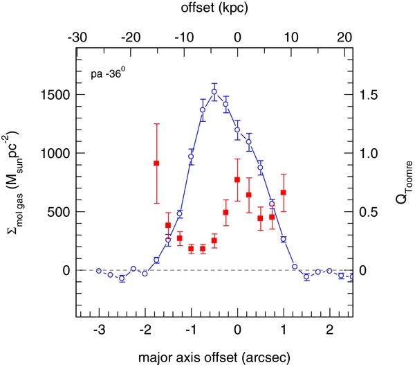
Figure 5. Molecular surface density (open blue circles) and Toomre Q-parameter (filled red squares, QToomre = (κσ0/πGΣmol gas)) in a 075 software slit along the major axis of the galaxy. Here κ is the epicyclic frequency, κ2 = R × d((v/R)2)/dR + 4 × (v/R), v is the rotation velocity at radius R, σ0 is the average local velocity dispersion (after removal of rotation and correction for instrumental resolution) and Σmol gas is the molecular gas surface density.
Download figure:
Standard image High-resolution imageThe expression used above for the Toomre parameter strictly applies only for the gas component. If the combined stellar and gas components are analyzed (Jog & Solomon 1984) and it is assumed, for simplicity, that the stellar and gas velocity dispersions are the same (because most of the stars were recently formed from the gas), the effective Q-parameter of the two-component system is smaller than Qgas by a factor χ ∼ (1 + f*/fgas), where f* is the stellar mass fraction. For z ∼ 1–2 SFGs gas and stellar fractions are comparable (χ ∼ 2; Tacconi et al. 2013) and the two-component system is even more gravitationally unstable.
3.2.2. Central Velocity Dispersion and Evidence for Star-forming Bulge
We observe significant kinematic anomalies in the data-minus-model residual maps of Figure 4. The largest anomalies are in the center of the galaxy in the dispersion residual map, and in the southern extension of the galaxy in both velocity and velocity dispersion residual maps (in both CO and Hα data; see Section 3.2.3). The central maximum in the residual velocity dispersion is significantly larger than expected from the beam-smeared rotation in an exponential disk galaxy with inclination 60°. Reducing the inclination decreases the beam-smeared velocity dispersion residual somewhat (because of the assumption of isotropic velocity dispersion in a thick disk) but does not eliminate the effect, unless an unrealistically low inclination is adopted.
A more likely explanation is a mass profile that is more concentrated mass distribution than the exponential disk profile assumed in the modeling of Figure 4. Such a mass concentration would be consistent with the presence of a substantial bulge component, which is also suggested qualitatively by the appearance of the dereddened stellar surface density map (bottom right panel in Figure 2). An R1/2 = 6.3 kpc exponential disk of total mass 3 × 10¹¹ M☉ (gas and stars) would have 2 × 10¹⁰ M☉, or 7% of its mass, within the central R ⩽ 1.5 kpc (018). The inferred stellar mass fraction within that radius deduced from the bottom right panel of Figure 2 is twice as large, or 14%. Within 04 (3.4 kpc) the exponential model would have 23% of the total mass, while the inferred stellar mass is 36%, which places EGS 13011166 among the "mature bulgy" systems in the M(⩽04)/Mtot versus [N ii]/Hα diagram of Genzel et al. (2008). Assuming that the mix of dust and gas is radially constant, this corresponds to a total baryonic mass of ∼4 × 10¹⁰ M☉ within R = 1.5 kpc. For an isothermal distribution, this mass would result in a velocity dispersion of 240 km s−1 at that radius, in agreement with the observed dispersion in the bottom left panel of Figure 4. We conclude that EGS 13011166 has a substantial nuclear bulge. Since the dereddened star formation rate peaks there as well, the bulge is actively star forming.
3.2.3. Evidence for Minor Merger and Clumps
There is a significant extension of the main body of the galaxy to the south, at a radius of ∼19 kpc, visible in the UV/optical, Hα, and CO maps, and with two prominent embedded clumps (labeled "C" and "D" in Figure 1). This velocity of this component is offset by +130 km s−1 with respect to the extrapolated disk velocity in this direction. It is thus quite likely that the southern component is due to an ongoing interaction or minor merger. If so, the companion has a 1:10 mass star formation rate ratio with respect to the main galaxy, as derived from the spatially resolved SED modeling. The ratio of molecular gas mass to star formation rate of this southern companion is similar to that of the main galaxy, corresponding to a depletion timescale of 0.3–1 Gyr, consistent with a normal star-forming galaxy.
There are three other prominent UV/optical clumps north, east, and southeast of the galaxy, at similar radii (Figure 1). CO is only marginally detected in the eastern clump ("B") at a velocity of −410 km s−1 relative to systemic, while CO emission spikes toward "A" and "E" are not statistically significant. It is thus not clear whether these clumps are part of the EGS 13011166 system.
3.2.4. Comparison of CO and Hα Kinematics
The line profiles, velocity channel maps, major axis velocity, and velocity dispersion profiles of the CO and Hα data are compared in Figure 6. They exhibit a remarkable agreement. This is notwithstanding the facts that the Hα-integrated map and the channel maps exhibit a tendency for the near-systemic Hα emission to be located east of the CO emission at these velocities, and for the southeastern CO maximum to be less prominent and further northwest in the Hα data. These findings are plausibly consistent, however, with the overall east–west color and extinction gradients discussed in Section 3.1.
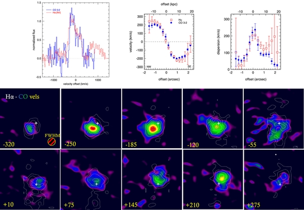
Figure 6. Comparison of CO and Hα data at the same resolution of FWHM 075. The top left panel is a comparison of the integrated, normalized CO (blue) and Hα (red) spectral profiles, with an instrumental resolution of FWHM 22 km s−1 (CO) and 100 km s−1 (Hα). The bumps at +940 and −670 km s−1 in the Hα spectrum are due to [N ii]. Top central and right panels: velocity dispersion and velocity (and ±1σ error) in a software slit of 1'' width, from Gaussian fitting along the major kinematic axis (position angle 36° west of north) in CO (blue) and Hα (red). Central and bottom rows: velocity channel maps (width ∼65 km s−1) in Hα (contours) and CO (color), sampled onto a 006 pixel−1 grid.
Download figure:
Standard image High-resolution imageThe agreement in molecular and ionized gas kinematics supports the interpretation that, at least in this massive SFG, both tracers can be equally well used for establishing the rotation curve and the galaxy kinematics. Where measurable with significance, the very good agreement of the intrinsic CO and Hα velocity dispersions in the outer parts of the galaxy along the major axis, where beam smearing effects should be minimum, supports the general conclusion mainly from Hα work that the interstellar gas layer in high-z SFGs is highly turbulent (σ0 ∼ 50–60 km s−1), and high-z disks thus are necessarily geometrically thick (hz/R ∼ σ0/vrot ∼ 0.15–0.3; Genzel et al. 2006, 2011; Förster Schreiber et al. 2009). The results presented here for a resolved case suggest that this conclusion holds for the entire star-forming interstellar matter (ISM) and not just its ionized component (see also Tacconi et al. 2013 for several other cases in PHIBSS).
3.3. The Spatially Resolved Molecular Gas–Star Formation Rate Relation
As explained in Section 1, our primary motivation for collecting such detailed CO, Hα, and HST observations in this galaxy was to study quantitatively the z > 1 molecular gas to star formation rate relation with spatially resolved data. The galaxy-integrated gas depletion timescale of EGS 13011166, τdepl = Mmol gas/SFR = 0.69 Gyr (Table 1), is identical with the average depletion timescale of z ∼ 1–1.5 MS SFGs (Tacconi et al. 2013).
To explore the spatially resolved KS relation, we grid the CO and HST data on a 025 × 025 pixel scale, oversampling the original LUCI Hα data by 50%. In Figure 7, we compare the inferred molecular gas surface densities (from Gaussian fitting to the CO data) to the effective screen extinction values inferred from the HST spatially resolved SED modeling, and smoothed to the same 075 FHWM resolution. The left panel of Figure 7 shows the overlay of these maps, with good qualitative agreement between the inferred optical extinction and the total molecular column, as noted before in Section 3.1.
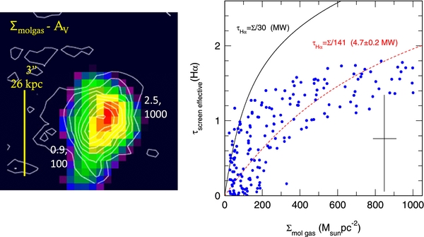
Figure 7. Comparison of effective screen extinction, as inferred from SED analysis of the four-band HST images, and the CO molecular gas mass surface density Σmol gas. Left panel: comparisons of the two-dimensional distributions (CO in white contours, A(V) in color) at the same FWHM resolution of ∼075, and sampled on a 025 grid. Right panel: pixel-by-pixel correlation between molecular column density (horizontal scale) and effective screen optical depth at Hα (τ(Hα) = 0.73 × A(V); Calzetti et al. 2000), with a typical uncertainty marked as a black cross. The black and dotted red curves are models for a homogenous mixture of gas, dust, and stars, where τeffective screen(Hα) = ln ((Σmol gas/30b)/{1 − exp (− (Σmol gas/30b))}), where b is the ratio of total molecular gas column to Hα optical depth in units of the diffuse Galactic ISM value (Σ/τ(Hα))MW ISM = 30 M☉ pc−2, or (N(H)/A(V))MW ISM = 2 × 1021 cm−2 mag−1 (Bohlin et al. 1978; see also Wuyts et al. 2011a; Nordon et al. 2013). The best-fitting curve has b = 4.7 ± 0.3, in good agreement with the findings of Nordon et al. (2013) for z ∼ 1–3 main-sequence galaxies observed in the UV, Herschel PACS, and CO.
Download figure:
Standard image High-resolution imageThe blue circles in the right panel of Figure 7 denote how these values compare quantitatively pixel by pixel. We note that the correlation of the data points is significantly better than what would be expected from the AV error bars obtained from pixel-by- pixel broadband continuum SED fitting (large cross). This is partly due to the correlation of sub-Nyquist-sampled data. More importantly, the extinction uncertainties include the impact of systematics stemming from varying star formation histories in the fitting procedure, etc., and thus—in a relative sense—are probably too conservative.
The observed correlation is nonlinear. It can be quite well modeled in terms of the conversion of a fully mixed distribution of gas and dust into the framework of an effective screen, where one would expect (e.g., Wuyts et al. 2011b)
where τeff and τtot are the effective screen and total dust optical depths along a given sightline. The total optical depth is related to the molecular column density through
where ΣMW = 30 M☉ pc−2 is the hydrogen column density of gas that is equivalent to a dust optical depth of unity in the R band in the diffuse ISM of the MW (at solar metallicity, N(H)/AV ∼ 2 × 1021 cm−2 mag−1; Bohlin et al. 1978). The dimensionless factor g then denotes how much this relation deviates empirically from the MW relation. The best-fit value of Equation (3) for the data in Figure 7 yields a value of g ∼ 4.8 ± 0.5. That is, the data in EGS 13011166, in terms of the mixed model in Equation (3), require a total dust to gas column ratio ∼5 times less than in the diffuse ISM of the MW. The fact that the data in Figure 7 seem to flatten even more than Equation (3) can accommodate, might suggest that g increases with Σmol gas.
Nordon et al. (2013) have recently investigated the relation between the ratio of far-infrared (FIR) to UV-flux densities and the UV SED slopes βUV in high-z SFGs. They also investigated the correspondence of these values to the total molecular columns as inferred from CO observations. Nordon et al. find from this totally independent approach that massive high-z SFGs are well described by a mixed dust/gas model with a ratio of effective UV-extinction to total UV column about five times smaller than expected from diffuse Milky Way ISM, which can be seen from the location of solar-metallicity main-sequence (MS) SFGs in the AIRX–βUV-plane (lower panel of their Figure 10, yielding ΔA/AIRX ∼ 5). This result is in good agreement with our findings.
The finding of a lower effective extinction to total gas column density ratio than in the solar neighborhood might at first seem contradictory to a solar or super-solar abundance ratio derived from the optical line ratios in Section 3.1.3. However, Nordon et al. (2013) have shown that this ratio is mainly dependent on the spatial distribution of gas and extinction, and not on the intrinsic gas to dust ratio.
3.3.1. KS Slope for a "Mixed" Extinction Correction
The success of this comparison encourages us to correct the observed Hα distribution, converted to a star formation rate, pixel by pixel with the AV map derived from the broadband SED fitting (using τHα eff = 0.73 × AV eff; Calzetti et al. 2000). Likewise, one can also use the molecular surface density distribution and then use Equations (3) and (4), with similar results. The resulting pixel-by-pixel relation between molecular gas and star formation rate surface densities is shown as green open squares (with 1σ uncertainties) in the left panel of Figure 8. Black filled circles give weighted averages (and their dispersions) of the same data, binning the green points in groups of 10–30. In following up on the likely overestimate of the AV errors in the SED fitting, we have assumed here that the (relative) AV errors are half those estimated from the SED fitting. A fit of the 110–170 data points in this plot (weighted by the uncertainties of the individual data points), depending on choices of significance cutoffs, etc., yields a slope of N = 1.14. The 2σ–3σ sensitivity of the CO measurements corresponds to gas columns of 100–200 M☉ pc−2, which we applied as cutoffs for the data considered. The statistical fit uncertainty is ±0.05 and the systematic uncertainty is about ±0.1, ..., ±0.15. With this modeling, the slope of the z ∼ 1.5 molecular KS relation is slightly above unity, in good agreement with the galaxy-integrated analysis presented in Tacconi et al. (2013) for 50 z = 1–1.5 SFGs, and with the radial aperture analysis of Freundlich et al. (2013) in four z = 1–1.5 SFGs.

Figure 8. Spatially resolved molecular KS relation in EGS 13011166. Left panel: green circles (and ±1σ uncertainties) denote CO-inferred molecular gas surface densities (horizontal) and the mixed-extinction/effective single screen corrected Hα-star formation rates (with a "single Calzetti" screen; Calzetti et al. 2000) for each 025 × 025 pixel in the map. Black filled circles and crosses denote the weighted binned medians of the individual pixel values and their dispersions. The dotted black line is the best-fit weighted linear regression to the green data, which yields a slope N = 1.14 ± 0.1. Right panel: binned weighted medians of the KS relations for other extinction correction methods: filled black circles denote the mixed case for an effective single Calzetti screen (N = 1.14 ± 0.1; the same as in the left panel); crossed red squares denote the global extinction correction method (N = 0.8 ± 0.05); the filled cyan squares mark a "double Calzetti" screen correction with an extra factor 2.27 for the nebular over the stellar extinction (N = 1.7 ± 0.25); and open blue circles show the correlation for the direct broadband SED modeling (without using the Hα data) of the star formation rate surface density (N = 1.15 ± 0.15).
Download figure:
Standard image High-resolution image
3.3.2. KS Slope for Different Extinction Correction Methods
The inferred KS slope depends strongly on the method of the extinction correction applied to the spatially resolved data. This is demonstrated in the right panel of Figure 8, where the binned weighted averages are shown for different extinction correction methods.
- 1.The "single" Calzetti effective screen extinction correction of the last section (identical with a "mixed" extinction correction from the total gas column), for each pixel in the observed Hα luminosity map, SFRHα 0 (M☉ yr−1) = exp(0.73 × AVeff) × L(Hα)obs/2.1e42 (erg s−1) (K98);
- 2.A single value ("global") extinction correction (11.4) of the observed Hα luminosity map, converted to star formation rate with SFRHα global (M☉ yr−1) = 11.4 × L(Hα)obs/2.1e42 (erg s−1) (K98). This method corrects the integrated star formation rate inferred from the observed Hα luminosity (33 M☉ yr−1) to the "true" total star formation rate, inferred from the sum of the observed UV-luminosity (23 M☉ yr−1), and the Herschel-PACS FIR luminosity (352 M☉ yr−11: PEP survey of Lutz et al. 2011, SFR(UV+IR) = 1.09 × 10⁻¹⁰ × (L(IR) + 3.3 × L(2800)); Wuyts et al. 2011a);
- 3.A "double" Calzetti effective screen extinction correction for each pixel in the observed Hα luminosity map, SFRHα 00 (M☉ yr−1) = exp(2.27 × 0.73 × AVeff) × L(Hα)obs/2.1e42 (erg s−1) (K98). This method is motivated by the finding in local starburst galaxies that the nebular gas has 2.27 times greater extinction than the stars (Calzetti et al. 2000);
- 4.Finally, a single "broadband" Calzetti screen extinction correction, as in Method 1, but for the star formation rate inferred from the broadband UV/optical SED modeling (Section 2.4).
In the right panel of Figure 8, the binned results for Method 1, "mixed" correction, are again (as in the left panel) shown as filled black circles (N ∼ 1.14). Method 4, the "broadband" correction, yields a similar slope of N ∼ 1.15 (open blue circles). For Method 2, the "global" correction, the slope of the resulting relation is flatter (N ∼ 0.8, crossed red squares). Method 3, the "double Calzetti" correction of the Hα data, yields the steepest slope (N ∼ 1.7, cyan).
Naturally, these different extinction correction methods also result in quite different integrated star formation rates. While the "single effective screen/mixed" correction perhaps is the most plausible method, given Figure 7, it delivers an integrated star formation rate of ∼114 M☉ yr−1, a factor three below the "ground-zero" star formation rate. In contrast, the "double Calzetti" correction yields ∼560 M☉ yr−1, or a factor 1.5 above the "ground-zero" value. The spatially resolved SED-fitting method yields an even-integrated star formation rate of 950 M☉ yr−1, a factor 2.5 too large. By design, the "global" correction matches the true value of 375 M☉ yr−1.
Clearly spatially resolved data as presented in this paper require a better empirical description of the spatially variable extinction component, which comes from a mixture of dust distributed diffusely throughout the galaxy, as well as dust located in the individual star formation regions. The former will correspond to the "single Calzetti/mixed" correction estimated from the broadband SED fitting. The latter may perhaps better be described as a constant average extinction (for each star formation region), rather than an extra extinction scaling with the diffuse screen correction, as in the "double Calzetti" recipe (S. Wuyts et al. in preparation; Nordon et al. 2013). In some cases, spatially resolved maps of the Hα/Hβ Balmer decrement may give a direct, spatially resolved measure of the extinction of the nebular gas.
Alternatively, one could observe a spatially resolved tracer of the obscured star formation. A "true" star formation estimator then is the sum of this and the observed Hα star formation rate, similar to the methods applied in the local universe (Kennicutt & Evans 2012; Kennicutt et al. 2009; Calzetti et al. 2007, 2010). An obvious tool is submillimeter continuum imaging with ALMA, which corresponds to the rest-frame FIR dust emission peak in high-z SFGs.
The inferred slope of the gas–star-formation relation also depends on the CO-molecular gas conversion factor. For simplicity, we have adopted a constant, MW conversion factor (αCO = 4.36 M☉ (K km s−1 pc2)−1 and a constant 1–0/3–2 brightness temperature ratio of 2. For near-solar metallicity SFGs there is observational and theoretical evidence that the conversion factor and the 1–0/3–2 ratio drop with increasing gas and star formation rate surface density (Tacconi et al. 2008; Genzel et al. 2010; Bolatto et al. 2013). Including these trends would have the tendency to increase the slope of the KS relation for all extinction correction methods discussed above.
4. SUMMARY
We have reported a comprehensive data set on the massive star-forming galaxy EGS 13011166 near the main star formation sequence at the peak of galaxy formation (z ∼ 1.5), combining resolution matched imaging spectroscopy and kinematics of molecular (CO 3–2) and ionized (Hα) gas components, and high-resolution four-band rest-frame UV to optical HST imagery.
- 1.In the short wavelength bands, the light distribution is characterized by a highly asymmetric and clumpy appearance spread over almost 40 kpc, similar to many other near-MS z > 1 SFGs. UV/optical colors exhibit strong spatial variations and are the result of extinction variations that correlate well with the molecular gas column density distribution inferred from the CO 3–2 map.
- 2.In contrast, extinction-corrected stellar mass and star formation rate distributions and the remarkably similar CO/Hα velocity distributions are smoother. The main body of the galaxy appears to be a large (R1/2 ∼ 6.3 kpc), inclined rotating disk, plus a massive (log M ∼ 10.6), star-forming central bulge.
- 3.The disk has a Toomre Q-parameter below unity and thus is globally unstable to fragmentation on the scales we have been probing.
- 4.The CO/Hα velocity distribution suggests that the southern extension of this disk may be a smaller (1:10) galaxy currently interacting or merging with the massive main system (log M = 11.5). A few of the other bright extra-disk clumps may also be part of the same galaxy group.
- 5.The nonlinear pixel-by-pixel correlation between the molecular gas column density and the effective extinction, inferred from SED modeling of the high-resolution HST data, is quite well modeled by a "mixed" dust/gas-stars model in which the ratio of total gas to dust column is about five times smaller than in the diffuse ISM of the MW.
- 6.The inferred slope of the spatially resolved KS relation is broadly consistent with those found in the local Universe (N ∼ 1–1.5), but the detailed value, and thus also the resulting extinction corrected star formation rate, strongly depends on the adopted extinction model and whether the CO conversion factor depends on gas surface density. To overcome this fundamental limitation in future work, it will be necessary to map a direct probe of the nebular extinction (via the Balmer decrement) or to obtain a tracer of the obscured star formation. An obvious tool is submillimeter continuum imaging with ALMA.
The observations presented here would not have been possible without the diligence and sensitive new generation receivers from the IRAM staff—for this they have our highest admiration and thanks. We also thank the astronomers on duty and telescope operators for delivering consistently high quality data to our team. We also thank the LUCI team and the staff of the Large Binocular Telescope Observatory for their support of these observations. A.D.B. acknowledge partial support from a CAREER grant NSF-AST0955836, and from a Research Corporation for Science Advancement Cottrell Scholar award. This work is based on observations taken by the CANDELS Multi-Cycle Treasury Program with the NASA/ESA HST, which is operated by the Association of Universities of Research in Astronomy, Inc., under NASA contract NAS5-26555.
Footnotes
- *
Based on observations with the Plateau de Bure millimetre interferometer, operated by the Institute for Radio Astronomy in the Millimetre Range (IRAM), which is funded by a partnership of INSU/CNRS (France), MPG (Germany), and IGN (Spain). Based also on data acquired with the Large Binocular Telescope (LBT). The LBT is an international collaboration among institutions in Germany, Italy, and the United States. LBT Corporation partners are LBT Beteiligungsgesellschaft, Germany, representing the Max-Planck Society, the Astrophysical Institute Potsdam, and Heidelberg University; Istituto Nazionale di Astrofisica, Italy; The University of Arizona on behalf of the Arizona University system; The Ohio State University, and The Research Corporation, on behalf of the University of Notre Dame, University of Minnesota, and University of Virginia.
- 18
In all these studies and throughout this paper, it is assumed that the conversion factor from CO 1–0 luminosity to molecular gas mass is the same as in the Milky Way (XCO = 2 × 1021 cm−2 (K km s−1)−1, or αCO = 4.36 M☉ (K km s−1 pc2)−1 (e.g., Genzel et al. 2010; Bolatto et al. 2013). This value and the resulting molecular depletion timescale include an upward 1.36 correction of the molecular hydrogen masses for the presence of helium.