


ABSTRACT
The origin of the high-energy component in spectral energy distributions (SEDs) of blazars is still something of a mystery. While BL Lac objects can be successfully modeled within the one-zone synchrotron self-Compton (SSC) scenario, the SED of low-peaked flat spectrum radio quasars is more difficult to reproduce. Their high-energy component needs the abundance of strong external photon sources, giving rise to stronger cooling via the inverse Compton (IC) channel, and thus to a powerful component in the SED. Recently, we have been able to show that such a powerful inverse Compton component can also be achieved within the SSC framework. This, however, is only possible if the electrons cool by SSC, which results in a nonlinear process, since the cooling depends on an energy integral over the electrons. In this paper, we aim to compare the nonlinear SSC framework with the external Compton (EC) output by calculating analytically the EC component with the underlying electron distribution being either linearly or nonlinearly cooled. Due to the additional linear cooling of the electrons with the external photons, higher number densities of electrons are required to achieve nonlinear cooling, resulting in more powerful IC components. If the electrons initially cool nonlinearly, the resulting SED can exhibit a dominant SSC over the EC component. However, this dominance depends strongly on the input parameters. We conclude that, with the correct time-dependent treatment, the SSC component should be taken into account in modeling blazar flares.
Export citation and abstract BibTeX RIS
1. INTRODUCTION
Combined as blazars, flat spectrum radio quasars (FSRQs) and BL Lacertae objects are the most violent subgroup of active galactic nuclei from Earth's point of view in the accepted unification scheme (Urry & Padovani 1995). The broadband spectral energy distribution (SED) of blazars is dominated by two broad non-thermal components. The low-energetic one, peaking usually between the infrared and the X-ray parts, is attributed to synchrotron radiation of highly relativistic electrons, while the process behind the high-energy component, peaking in the γ-rays, is a matter of ongoing discussion.
Although a hadronic origin is a possibility (e.g., Mannheim 1993) for the high-energetic component, most authors favor a leptonic origin of the γ-radiation (for recent reviews see Böttcher 2007, 2012). If highly relativistic electrons (and also positrons) interact with an ambient photon field, the photons can be inverse Compton (IC) scattered to very high energies. Such photon fields can be the synchrotron photons of the same population of electrons (the so-called synchrotron self-Compton (SSC) effect; Jones et al. 1974), or photon sources external to the jet (the so-called external Compton (EC) models), such as photons directly from the accretion disk surrounding the black hole in the center of the active galaxy (Dermer & Schlickeiser 1993), from the broad line regions (Sikora et al. 1994), or the dusty torus (Blazejowski et al. 2000; Arbeiter et al. 2002).
In particular the SEDs of FSRQs are dominated by the IC component, i.e., most of the luminosity of this type of blazar is emitted in the γ-rays (e.g., Hayashida et al. 2012 for 3C 279, or Vercellone et al. 2011 for 3C 454.3). Since one can measure several thermal emission components in FSRQs, the EC process seems to be a natural choice to model the SED. Being able to detect unbeamed thermal emission, the strongly boosted non-thermal radiation of the jet notwithstanding proves the abundance of strong external photon fields. This in turn provides lots of seed photons for the electrons, which cool rather strongly by this process, giving rise to a powerful IC component.
On the other hand, BL Lac objects emit most of their power in the synchrotron component having at most comparable IC fluxes. In particular, high-frequency peaked BL Lac objects exhibit a much reduced γ-ray flux compared to the synchrotron flux. This points toward a main cooling by the synchrotron channel, and the SSC process is successfully used to model BL Lac objects (e.g., Acciari et al. 2011 for 1ES 2344+514, or Abramowski et al. 2012 for 1RXS J101015.9−311909).
However, such a strict division of the two blazar types has recently been called into question. Chen et al. (2012) performed a numerical analysis of the multiwavelength variability of the FSRQ PKS 1510−089. Using a time-dependent code they were unable to find a clear preference of the EC over the SSC process, and stated that the SSC process might even be preferable, since it matches the X-ray part of the SED far better than the EC process.
The advantage of the time-dependent numerical treatment over the usual steady-state approach is that such codes naturally implement the time-dependent nature of the SSC process, which is normally omitted in many theoretical investigations (e.g., Moderski et al. 2005; Nakar et al. 2009) and modeling attempts (e.g., Ghisellini et al. 2009; Aleksic et al. 2012). Consider an electron population that emits synchrotron radiation and then scatters this self-made radiation up to γ-rays. The electrons therefore lose energy, which means that the emitted synchrotron emission will also be less energetic, as will be the SSC emission. This implies that the cooling rate will also become weaker over time, i.e., the cooling rate is time dependent. Schlickeiser (2009) gave an analytical expression for the time-dependent SSC cooling rate, which is proportional to an energy integral over the electron distribution function itself.
Schlickeiser et al. (2010, hereafter referred to as SBM) combined the new SSC cooling term with the well-known synchrotron cooling term to give a more realistic treatment. As mentioned above, the SSC cooling becomes weaker over time, which means that after some time it will be weaker than the standard linear cooling terms, such as synchrotron cooling, since they do not depend on time. They also calculated the synchrotron SED with the remarkable result that the synchrotron component exhibits a broken power-law behavior. Interestingly, this feature is independent of the electron injection function. While SBM used a δ-like injection, Zacharias & Schlickeiser (2010) performed the same analytical calculation using a power-law injection. Apart from the high-energy end of the synchrotron component the broken power-law behavior is the same in both cases. This is due to the fact that any extended form of the electron distribution is rapidly quenched into a δ-like structure, as long as no reacceleration is taken into account. Therefore, the δ-approach is in someway a late-time limit for any extended injection.
Following up on the results described above, Zacharias & Schlickeiser (2012, hereafter referred to as ZS) calculated analytically for the δ-approach the emerging SSC SED. They obtained the interesting result that the time-dependent SSC cooling leads, in fact, to a dominant IC component without the need for extreme parameter settings. Additionally, they found that the SSC component exhibits a broken power-law, which may also be independent of the injection form.1
As we have already discussed above, the debate about whether SSC, EC, or both play an important role especially in FSRQs is not yet settled. Since we showed in ZS that a dominant SSC component is easily achievable, it is straightforward to include the EC scenario in our approach. Therefore, we will extend the loss rate of SBM with the additional contribution of the EC losses. This will be done in Section 2. In Section 3 we will calculate the resulting intensity and fluence spectrum of the EC component, where the fluence is the time integrated, i.e., averaged, intensity. The lengthy details of these calculations can be found in Appendices B and C. Transforming the results into the form of an SED will be done in Section 4, where we will also summarize the results of ZS for the sake of completeness. At the end of this section we will give some example SEDs with all contributions of synchrotron, SSC, and EC, and will discuss the results. In Section 5 we will summarize the results and present our conclusions.
2. THE EXTENDED LOSS RATE
Since we intend to calculate the spectrum due to EC emission, we have to include this type of energy transfer between electrons and photons in the energy loss rate of the relativistic electrons. According to Dermer & Schlickeiser (1993), the pitch-angle-averaged loss rate of electrons in an external photon field which is isotropically distributed in the lab frame is
with the speed of light c = 3 × 1010 cm s−1, the Thomson cross section σT = 6.65 × 10⁻²⁵ cm2, the energy of an electron at rest mec2 = 8.14 × 10⁻⁷ erg, the electron Lorentz factor γ, and the Lorentz factor of the radiating plasma blob Γb.
We assume that the energy density of the external photons is isotropic in the galactic (primed) frame and is given by
where L'ad is the luminosity of the accretion disk surrounding the central supermassive black hole, τsc is the scattering depth of the ambient medium scattering the accretion disk photons, and R'sc is the radius up to where the accretion disk photons are scattered by the ambient medium.
Adding the external cooling term to the synchrotron and SSC cooling terms, we obtain the complete electron loss rate:
with D0 = 4cσTuB/(3mec2) = 1.29 × 10⁻⁹b2 s−1, the magnetic energy density uB = B2/8π, and the magnetic field B = b G. Schlickeiser (2009) gives the constant A0 = 3σTc1P0R 20/(mec2) = 1.15 × 10⁻¹⁸R15b2 cm3s−1, which was obtained during the derivation of the time-dependent SSC cooling term. The parameters are given as P0 = 2 × 1024 erg−1s−1, 0 = 1.856 × 10⁻²⁰b erg, and c1 = 0.684. We scaled the radius of the spherical emission blob as R = 1015R15 cm.
The nonlinearity of the SSC cooling manifests itself in the integral over the volume-averaged electron distribution n(γ, t). The factor
shows the relative strength of external to synchrotron cooling. For lec ≫ 1 the linear cooling is dominated by the external photons, while for lec ≪ 1 the synchrotron process mainly operates. Apart from R'sc, which is scaled as R'sc = 3.08 × 10¹⁸Rpc' cm, we scale the quantities in Equation (4) as Q = 10xQx in their respective cgs units, and Γb = 10Γb, 1.
We can now formulate the differential equation describing the competition between the injection of ultrarelativistic particles with the source function S(γ, t) and the energy losses as described by Equation (3) inside the spherical emission region (Kardashev 1962):
In order to keep the problem simple, we assume a monoenergetic instantaneous injection S(γ, t) = q0δ(γ − γ0)δ(t). Inserting Equation (3) into Equation (5) we obtain
which apart from the factor (1 + lec) equals the differential equation that was solved by SBM. We can therefore use their solution. The only difference is that we have to insert the factor (1 + lec) wherever they have a D0. The solution is given in cases of the injection parameter α, which is proportional to the ratio of the nonlinear to linear cooling at the time of injection. We will discuss its implications in Section 2.1.
For dominating linear cooling (α ≪ 1), we get the electron distribution

If initially the nonlinear cooling dominates (α ≫ 1), we obtain
which is valid for times

For late times the linear cooling takes over and the distribution function is described by a modified linear solution:
2.1. The Injection Parameter α
We have written the solutions of the differential Equation (6) dependent on the parameter α, which we now intend to discuss in greater detail.
We call it the injection parameter, and it is defined as the square root of the ratio of the nonlinear cooling term to the linear cooling term at the time of injection, i.e.,
where N denotes the number of radiating particles, and we applied the same scaling law for the parameters as above.
For α ≪ 1 we see that the linear cooling dominates, resulting in the solution (7). If α ≫ 1, the nonlinear cooling at least initially dominates, giving the solutions (8) and (10) for early and late times, respectively. The time tc marks the transition from nonlinear to linear cooling.
Comparing the α given above to the injection parameter obtained by SBM (where EC losses were neglected), we find that
where αSBM = A0q0γ20/D0.
This implies that the contribution of the external photons lowers the possibility for nonlinear cooling. Solving Equation (11) for the electron density we obtain
This also demonstrates the aforementioned fact that with EC losses included it is harder to cool the electrons nonlinearly. Equation (13) shows that for the same value of α, i.e., the relative strength between linear and nonlinear cooling, one needs a higher electron density in the blob compared to the case where the external losses are neglected.
3. EXTERNAL COMPTON FLUENCE
The intensity due to IC collisions of electrons with external photons is given by

with the emissivity (see Appendix A)
where is the normalized target photon energy in units of the electron rest mass mec2, s is the normalized scattered photon energy, u() is the target photon density, and
being the Klein–Nishina cross section (Blumenthal & Gould 1970) with


Thus, we obtain for Equation (15)
Here

denotes the minimum Lorentz factor for the electrons, below which the electrons would gain energy from the photons.
The fluence is the time-integrated intensity spectrum, giving an average of the variability in all bands, and also incorporating that observation times can be much longer than the typical flare duration:
The intention of this paper is to calculate analytically the complete SED of blazars. We will therefore use the simplest approach possible for the external photon density in the comoving frame:
where ec is the normalized energy of the target photons in the comoving frame. Using the electron densities (7), (8), and (10) we can calculate the intensity, and subsequently the fluence.
3.1. Small Injection Parameter, α ≪ 1
Using Equation (7) in Equation (14) we find for the case of α ≪ 1:
after performing the simple integrations of the δ-functions and substituting τ = D0(1 + lec)γ0t. Here we define I0 = RcσTq0Γ2bu'ec/(4π2ecγ20),

Inserting Equation (25) into Equation (23) we obtain after some calculations (see Appendix B) the final expression for the EC fluence in the case of dominant linear cooling:
where F0 = I0/(D0(1 + lec)γ0) and cut = 4ecγ20/(1 + 4ecγ0).
In the Thomson limit Γ0 = 4ecγ0 ≪ 1 the spectrum cuts off at s ≈ Γ0γ0 ≪ γ0. The Thomson limit also implies that ec ≪ (4γ0)−1. Hence, there is no break in the spectrum, and the denominator in Equation (30) equals unity.
In the Klein–Nishina limit Γ0 ≫ 1 we find ec ≫ (4γ0)−1, and the cutoff at s ≈ γ0. Thus, the spectrum breaks at s = −1ec.
3.2. Large Injection Parameter, α ≫ 1
3.2.1. Early-time Limit, t ⩽ tc
For t ⩽ tc we use Equation (8) in Equation (14), as well as the same substitution for t as above, and obtain after solving the simple integrations
with τc = (α3 − 1)/3α2,
Using Equation (23) with Equation (31) the fluence for the early time limit can be calculated. The full details can be found in Appendix C. The solution depends on the external photon energy ec, giving three different cases.
For  we have
while for  we get
The last part is for  and becomes
Here we used γB = γ0/α, and  .
.
3.2.2. Late-time Limit, t ⩾ tc
As before, we can find the intensity for t ⩾ tc, if we insert Equation (10) into Equation (14). As in the previous cases we exchange t, and obtain
with
Inserting Equation (38) into Equation (23) one can obtain the fluence in the late-time limit. For details we again refer the reader to Appendix C. The results depend also on the external photon energy, giving two cases this time. For  we find
while for  we obtain a single power law in the form
3.2.3. Total Fluence in the Case α ≫ 1
Combining the results of the previous sections we obtain the total fluence for the IC component due to interactions with the ambient radiation field in the case where the electrons are at first cooled nonlinearly. We have three different cases depending on the value of the normalized external photon energy ec.
For  we find
Secondly, if  the fluence becomes
Finally, we obtain for 
These are all broken power laws, where at least one break ( ) depends strongly on the value of α, and therefore on the nonlinear cooling.
We note that the first case corresponds to the extreme Klein–Nishina limit (Γ0 ≫ 1), the second one to the mild Klein–Nishina limit (Γ0 > 1), and the last one to the Thomson limit (Γ0 ≲ 1).
4. THE COMPLETE SED
Using the results of the last section and of ZS,2 we are now in a position to present the complete SED in a combined picture of SSC and EC radiation. The IC component will therefore be the sum of the SSC and EC contributions. If these contributions are comparable on some scales, the resulting spectrum will deviate from a pure power law.
In order to present the results in a manner that can be easily compared to data, we will give the SEDs depending on the frequency ν' = (mc2/h)δ, which is already transformed to the frame of rest of the host galaxy with the Doppler factor  , where μobs is the cosine of the angle between the jet and the line of sight, and
  is the normalized speed of the plasma blob. The SED is then given by the fluence multiplied by the frequency f' = πcRν'F'(ν') in units of erg s−1 with the transformed fluence F' = δ4F.
We should note that we have to adapt the results of ZS to the case discussed here. That is, we have to include the addition of the EC cooling to the linear term. This can be done by replacing any "D0" of ZS with "D0(1 + lec)." Interestingly, the synchrotron component will not be affected by this replacement, while the SSC component gains a factor (1 + lec).
Below we will first present the theoretical SEDs and afterward give a brief discussion of the results.
4.1. Synchrotron SED
From Equation (ZS-69) we obtain the synchrotron SED for the case α ≪ 1, which is
with νsyn = 4.1 × 10¹⁴δbγ24 Hz.
The maximum value of the synchrotron SED,
is attained at
Using Equation (ZS-82) we can write the synchrotron SED for α ≫ 1 as
It peaks at
with the maximum value
4.2. Synchrotron Self-Compton SED
For α ≪ 1, ZS found two different versions of the SSC SED depending on the Klein–Nishina parameter K = 0.136bγ34. In the Thomson limit (K ≪ 1) we use Equation (ZS-72) and get
while for the Klein–Nishina limit (K ≫ 1) with Equation (ZS-73) we have
with the constants νT = 1.6 × 10²³δbγ44 Hz, the break frequency νB = 2.3 × 1024δb−1/3 Hz (Schlickeiser & Röken 2008), and  .
.
The maximum frequencies

and

imply the maximum values

and

respectively.
For the SSC SEDs in the case α ≫ 1 we have to discuss three different cases depending on the Klein–Nishina parameter K, and we begin with the Thomson limit (K ≪ 1) using Equation (ZS-85):
The maximum value

is attained at

For the mild Klein–Nishina limit (1 ≪ K ≪ α3) Equation (ZS-88) yields
This triple power law peaks at

and reaches a maximum value of
The last case is the extreme Klein–Nishina limit (1 ≪ α3 ≪ K). We obtain the SED from Equation (ZS-91), resulting in
The SED peaks with a maximum value
at a peak frequency
4.3. External Compton SED
In the case of α ≪ 1 the SED can be calculated from Equation (30), becoming
where νbr = 1.23 × 10²⁰δ−1ec Hz and νcut = 1.23 × 10²⁰δcut Hz. In the Thomson limit (ec ≪ (4γ0)−1) the maximum frequency

leads to a peak value of

In the Klein–Nishina limit (ec ≫ (4γ0)−1) the maximum value
is attained at
Now, we convert the results of Equations (44)–(46) into SEDs, which are the cases for α ≫ 1, yielding for the extreme Klein–Nishina limit 
with  and
and  . It peaks at

with a maximum value of

In the mild Klein–Nishina limit  , with
  , we obtain
The maximum value

is attained at
Finally, we have the Thomson limit  , where the SED becomes
It peaks at
(note that we use a different approximation for  , that is for
  , compared to Equation (78)) reaching a maximum value of

4.4. Discussion
In Figure 1 we present several model SEDs for different sets of parameters. Since the number of free parameters is fairly large, a strict parameter study is beyond the scope of this paper, although we will discuss some aspects below. Therefore, we use some global parameters, which are unchanged through all figures, namely, δ = 10, and Γb, 1 = L'46 = τ−2 = R'pc = R15 = 1. The normalized external photon energy is also fixed at ec = 10−4. This leaves us with three free parameters: the injection parameter α, the relative strength of the EC cooling lec, and the initial electron Lorentz factor γ0. These parameters are given at the top of the plots for each case.
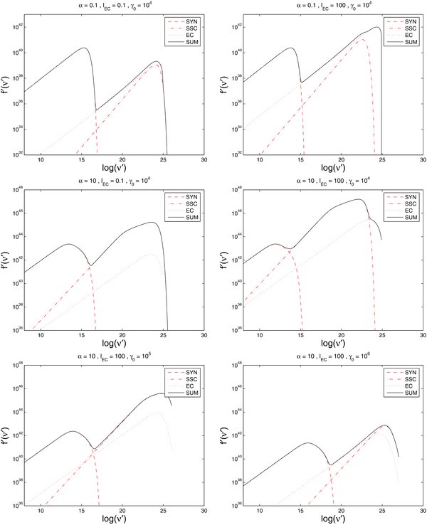
Figure 1. Model SEDs for several cases of α, lec, and γ0. Specific parameters are given at the top of each plot, while the global parameters are given in the text. Top row: α ≪ 1 in the Thomson limit for both cases of lec. Middle row: α ≫ 1 in the Thomson limit for both cases of lec. Bottom row: α ≫ 1 and lec ≫ 1 in the mild and extreme Klein–Nishina regime, respectively.
Download figure:
Standard image High-resolution image
Since we use lec as a free parameter and fix almost all parameters it contains, we get the magnetic field strength b as a dependent variable. Increasing lec results in a decreasing magnetic field. This choice also demonstrates that the figures given as examples here only cover a very narrow range of possible realizations.
We note that for the top panels of Figure 1 we use Equation (68) for the EC component, while we use Equation (79) in the middle plots and Equations (76) and (73) for the lower plots, respectively. This is due to our choice of parameters.
The first obvious result is that for α ≪ 1 the IC component is significantly influenced, if not dominated, by the EC component. For α ≫ 1 the main contribution comes from the SSC component, at least in the Thomson and mild Klein–Nishina limits. This is expected, since α controls the main cooling mechanism, which should also influence the SED.
Similarly, this is also correct if one considers the linear coolings only, where the relative strength is controlled by lec. For example, in the top plots of Figure 1, where we use Equation (68), one can see that for lec ≪ 1 the synchrotron component dominates the EC component, while for lec ≫ 1 it is the other way round. Since  , one could expect that the ratio of the peak values Rec, s = f'ec, max/f's, max∝lec. This is certainly true for the Thomson limit of Equation (68), as is shown in Equation (D2) of Appendix D. However, due to our choice of parameters the top panels of Figure 1 use the Klein–Nishina limit of Equation (68), where Equation (D3) demonstrates that the ratio is more involved and depends also on γ0 and ec. Using the parameters of the plots in the top row of Figure 1, we find that the ratios become Rec, s ≈ 0.07 and Rec, s ≈ 66, respectively, consistent with the plots.
In Appendix D we also show the ratios between the maximum values of the SSC and EC components. As one can see, every Rssc, ec∝(1 + lec)/lec, with the consequence that the ratio is independent of lec for lec ≫ 1. Although the dependence on other parameters is rather involved and changes from case to case, we can say that a lower value of the external photon energy ec favors the EC component, while a higher value of the injection parameter α favors the SSC component, as one would expect.
On the other hand, if lec ≪ 1, we find Rssc, ec∝l−1ec. This implies that the EC component is much reduced compared to the SSC component. This is also expected, since in this case the EC cooling is the weakest operating mechanism, if the other parameters are chosen accordingly. It is, of course, still possible that SSC could be lower than EC, since the ratios in Appendix D can always become smaller than unity.
As one can see in the lower panels of Figure 1, we achieve similar results in the mild and extreme Klein–Nishina regimes. In particular, in the latter case, we have an example where the inclusion of the EC cooling has significant effects on the emerging spectrum, giving a different power law and peak value compared to the case where either EC or SSC is neglected.
As stated above, in Figure 1 we just show some model plots with only a very limited range of application, since we fixed most of the free parameters. Some of them, however, might have a significant impact on the resulting SED, such as the radius R of the plasma blob, which we set to R15 = 1. This value corresponds to a light crossing timescale of tlc = R/(δc) ≈ 0.9h (with δ = 10), which is usually equal to the variability timescale tvar of the source. Naturally, a broad range of variability timescales is observed in blazars, ranging from minutes (as in the cases of PKS 2155−304, Aharonian et al. 2007 and PKS 1222+216, Tavecchio et al. 2011) to months (e.g., Abdo et al. 2010), indicating a large range of possible radii for the emission blobs.
Increasing the radius of our plasma blob would result in a decreasing value of the injection parameter, since α∝R−1 according to Equation (11). This implies that the SSC component would become less important, leading to a dominant EC flux in the high-energy regime.
On the other hand, long variability timescales can also be the result of inefficient cooling or other factors with long timescales, such as a rotating jet (e.g., Agudo et al. 2012). Our simple model assumes an instantaneous and effective cooling of the electrons far from steady state, favoring short variability timescales, at least if one is interested in the effects of nonlinear SSC cooling. Schlickeiser (2009) as well as Zacharias & Schlickeiser (2010) showed that the nonlinear process begins orders of magnitudes earlier to cool the electrons than the standard linear synchrotron cooling, implying shorter variability timescales. However, a true analysis of the variability should be performed with the help of light curves, which we aim to present in another paper.
We should also note that our discussion adopts a point-like emission zone, which means that we neglect additional effects from photon retardation variability processes from the finite size of the emission zone. For an extended analysis of these effects we refer to the discussion in Eichmann et al. (2010, 2012).
Another parameter, which might easily have different values, is the Doppler factor δ. In the literature it usually covers a range 10–30, but extreme values of 50 and higher have been used to model blazar spectra (e.g., Begelman et al. 2008), although the latter are mostly regarded as unrealistic.
For our plots we used δ = 10. Increasing that value would not change the overall appearance of the SED, since in our simple model the dependences on δ are the same in all cases; however the peak luminosities would increase significantly. In the plots in Figure 1 we achieve γ-ray luminosities roughly between 1039 erg s−1 and 1046 erg s−1. The former value is rather low for blazars. However, the values of the peak luminosity depend strongly on the parameters, which might differ from the ones used to create the plots.
As an example: with δ = 50, α = 50, and lec = 100 one would arrive at an SSC luminosity of roughly 1050 erg s−1. This is close to the highest recorded luminosity of blazars, achieved by 3C 454.3 with a peak luminosity of 2.1 × 1050 erg s−1 (Abdo et al. 2011b). In principle, the above-stated values for α and lec could be achieved by setting N50 ≈ 120 and b = 0.14. The high number of electrons in the source may not be that unrealistic, since a large outburst requires something extreme going on, such as a large mass load into the jet. According to Equation (61) the peak frequency of the SSC component would be at roughly 3 × 10²³ Hz, which is reasonable (Abdo et al. 2011b). Using Equation (51) we obtain a synchrotron peak frequency roughly at 8 × 10¹¹ Hz, which is in the far-infrared regime. Still, a Doppler factor of 50 is quite high, severely questioning the validity of the results of our simple model. Only a detailed spectral analysis, potentially also including a discussion of variability aspects (see above), can decide about the validity. However, such an analysis is beyond the scope of this paper.
Another important aspect is the energy transported and dissipated by the content of the jet. The initial comoving energy density of the electrons is given by ue = q0γ0mec2. Using Equation (13), we obtain
The power transported by these electrons is given by  , yielding with
A widely used measure to quantify whether the jet is dominated by particles or the magnetic field is the equipartition parameter
which can be rewritten with the help of Equation (4), giving

Table 1 lists the values of these constraints for the plots given in Figure 1. Depending on the parameters used we obtain a wide range of possible realizations.
Table 1. Energetic Estimates of the Plots in Figure 1
| Plot | ue | Pe | ue/uB |
|---|---|---|---|
| (erg cm−3) | (erg s−1) | ||
| TL | 9.1 × 10⁻⁴ | 9.2 × 1039 | 3.0 × 10⁻² |
| TR | 9.1 × 10⁻² | 8.5 × 1041 | 2.4 × 10³ |
| ML | 9.1 | 8.9 × 1043 | 2.7 × 10² |
| MR | 9.1 × 10² | 8.5 × 1045 | 2.5 × 10⁷ |
| LL | 91 | 8.5 × 1044 | 2.5 × 10⁶ |
| LR | 9.1 | 8.5 × 1043 | 2.5 × 10⁵ |
Notes. TL: top left; TR: top right; ML: middle left; MR: middle right; LL: lower left; LR: lower right.
Download table as: ASCIITypeset image
A first result is that we are far from equipartition with all our setups, and only the case with the lowest energies involved shows a dominant magnetic field. This is reasonable, since the number of electrons in this case is also at a minimum in our models. This is also the only case where the synchrotron peak dominates the IC peak. However, we should note that this might be an artifact of our parameter settings, i.e., the inverse dependence of b on lec, while we left all other parameters in lec unchanged. Keeping b at some value and changing some other parameters in lec might give a different picture.
The energy density ue and the transferred power Pe of the electron naturally increase with the number of particles in the blob. Comparing our values of Pe with, e.g., those of Ghisellini et al. (2009), we find that our plots cover a range that is usually below the obtained values for FSRQs, which is again due to our choice of parameters. The case with α = 10, lec = 100, and γ4 = 1 is, however, exactly in the range obtained by these authors. Higher values, as we used for the discussion about 3C 454.3 above, are also possible. So, from the energetics point of view our model is definitely supported.
5. SUMMARY AND CONCLUSIONS
In this paper we aimed to extend the earlier work of Zacharias & Schlickeiser (2012, ZS) regarding the importance of time-dependent SSC cooling scenarios for modeling the SEDs of blazars.
In ZS we were able to give an analytical SED for a pure synchrotron/SSC picture. However, especially in the context of FSRQs, a preference is given in the literature to EC scenarios, where the high-energy component is modeled using external photon sources that are IC scattered by the jet electrons. We considered this effect here by introducing the EC cooling term into the differential equation describing the time- and energy-dependent behavior of the electron distribution function. We used a rather simple model, where we assumed the external photons to be isotropically distributed in the frame of the blob. This is justified by our intention to show in an analytical demonstration the possibilities and differences of our approach compared to the usual steady-state approach. More realistic scenarios can mostly be treated only numerically, since they contain more sophisticated assumptions and effects.
We then calculated the resulting EC intensity, the fluence, and eventually the SED. Adapting the results of ZS regarding the synchrotron and the SSC SED, we have now obtained a complete analytical prediction of the appearance of blazar SEDs, if the electrons are cooled by the nonlinear, time-dependent SSC channel in combination with the linear synchrotron and EC channels.
The main addition to the conclusions of ZS is that which type of cooling dominates critically depends on the parameters of the source. For only weak EC cooling the results of ZS are recovered, while in the other case the shape of the high-energy component can change significantly. In Appendix D we calculate the ratios of the maximum values of each component with the other components, since they mark the dominance of one component over the others. These ratios especially show the importance of the choice of the specific values of the parameters and demonstrate that a broad range of realizations is possible.
We also note that the nonlinear cooling has significant effects on the shape of the spectrum of all components leading to additional and also unique breaks, which strongly depend on α. This highlights once more the severe effects of the time-dependent treatment.
To conclude, we can say that our investigation so far has clearly shown the importance of the inclusion of the time-dependent nature of the SSC cooling term, especially in blazar flaring states, which are far from steady state. The resulting spectra differ significantly from the usual approach, where these effects are not taken into account. Secondly, due to the broad range of free parameters in the EC model, the SSC component should not be dismissed beforehand while modeling blazars. As we were able to show here, the SSC component might be as important as the EC component, if the correct time-dependent treatment is applied, which is especially necessary in flaring states.
In order to quantify the differences between the time-dependent and steady-state approaches somewhat further we intend to calculate the resulting light curves and discuss the effects of optical thickness in a future work. The former might show in a clearer form that the SSC cooling actually acts a lot more quickly than the usual cooling scenarios, while the latter might be important to constrain the free parameters, such as the Doppler factor.
We thank the anonymous referee for constructive and detailed comments, which helped significantly in improving the manuscript. We acknowledge support from the German Ministry for Education and Research (BMBF) through Verbundforschung Astroteilchenphysik grant 05A11PC1 and the Deutsche Forschungsgemeinschaft through grant Schl 201/23-1.
APPENDIX A: THE EXTERNAL COMPTON EMISSIVITY
According to Dermer & Schlickeiser (1993) the general emissivity due to EC scatterings is given by
where Ω and Ωe mark the direction of the incoming photon and the electron, respectively, and cos Ψ = μμe + (1 − μ2)1/2(1 − μ2e)1/2cos (Φ − Φe) is the angle between the incident photon and the electron.
Assuming complete isotropy we can write u(, Ω) = u()/4π, n(γ, Ωe) = n(γ)/4π, and σ(s, , γ, Ω, Ωe) = σ(s, , γ)/4π. Plugging this into Equation (A1) the angle integrations can be easily performed, yielding

which agrees with Equation (15).
APPENDIX B: INTENSITY AND FLUENCE FOR α ≪ 1
Using Equation (7) in Equation (14) we find for the case of α ≪ 1:

which leads directly to Equation (25) with the substitution τ = D0(1 + lec)γ0t and the definition I0 = RcσTq0Γ2bu'ec/(4π2ecγ20).
Integrating Equation (25) with respect to time yields

where we set F0 = I0/(D0(1 + lec)γ0).
Inverting q(τ) gives

This can be substituted into Equation (B2), yielding

With the above substitution the function G simplifies to

The final substitution x := (secq)−1 gives

This integral cannot be solved in closed form. However, we can achieve approximative results giving reasonable solutions for most of the parameter space.
For s < −1ec one can see that both integration limits are much larger than unity, and so is x. Thus, we can approximate the fraction
The bracket in Equation (B6) is to leading order in this approximation G(x) ≈ 1. Now, this can be easily integrated, yielding

For s > −1ec and  both integration limits are smaller than unity and the fraction in the integral of Equation (B6) becomes
The leading order of G(x) is here G(x) ≈ 2/(secx2). The integral, thus, results in

For intermediate frequencies  we can split the integral into two regimes and use the above approximations:

Combining the above results we obtain the final expression for the EC fluence in the case of dominant linear cooling:
where cut = 4ecγ20/(1 + 4ecγ0) is the solution of the equation s/(4ecγ0(γ0 − s)) = 1, yielding Equation (30).
APPENDIX C: INTENSITY AND FLUENCE FOR α ≫ 1
C.1. Early-time Limit, t ⩽ tc
For t ⩽ tc we use Equation (8) in Equation (14) and obtain

Using the same definitions of τ and I0 one can easily arrive at Equation (31). Then, the fluence integral can be written as

Examining the Heaviside functions we find that τc is the upper limit as long as  , while for
  the upper limit becomes [(γ0/γmin)3 − 1]/3α2. As long as they are not really needed we will refer to both of them as the respective variable with the subscript up.
The break energy is given by
where γB = γ0/α.
Substituting μ = (1 + 3α2τ)1/3 we obtain
where  and
and  .
.
Inverting q(μ) yields
Inserting this into Equation (C4) with  and
and  , we find

Using again the substitution x = (secq)−1 we eventually obtain

with the lower limits  and
and  .
.
Since this integral cannot be solved in closed form either we will now consider similar approximations as in the linear case. Additionally, we will now consider each case of the lower limit in turn.
Beginning with  we use the lower limit
  . In case of
  we find for
  that both limits are lower than unity and we approximate the fraction in Equation (C7) with
and G(x) becomes to leading order G(x) ≈ 2/(secx2). Hence,

For  we see that the upper limit is larger than unity, while the lower limit is still smaller than unity. We will therefore split the integral. For the part below unity we use the above-mentioned approximation, while for the part larger than unity we approximate the integrand with x−7/2. Thus,

Combining the last two equations we obtain
For  we can make use of Equations (C9) and (C10), while x ≪ 1 and x ≈ 1, respectively, yielding

and
If both limits are larger than unity we approximate the integrand with x−7/2 and obtain

Combining the Equations (C12)–(C14) we can write the final result as

Now, we turn our attention to the case where  , which means that the lower limit in the integral of Equation (C7) becomes xdown = 4γ0(γ0 − αs)/2sα2.
The first thing we notice is that the upper limit is always larger than unity. This is also true for the lower limit, except for  . In the latter case, we obtain with the same approximations as above

In the case where both limits are larger than unity, we find

Finally, we can give the fluence in the early-time limit covering all energies. However, we have to distinguish three cases for the external photon energy.
For  we have

while for  we get

The last part is for  and becomes

C.2. Late-Time Limit, t > tc
As before, we can find the intensity for t ⩾ tc, if we insert Equation (10) into Equation (14):

Equation (38) is recovered if one uses the definitions of τ and I0, again. The fluence then follows as

Substituting y = ((1 + 2α3)/3α2) + τ we obtain

Inverting q(y) gives  , which leads to

Finally, we use again x = (ecsq)−1 and thus the fluence becomes

As before, we will consider approximative results. For  both limits are smaller than unity, and we approximate the integrand with (23secx2)−1 giving

For  both limits are larger than unity and the integrand can be written as x−5/2, yielding

In the intermediate part  we can use both limits to obtain

Collecting terms, we find the fluence in the late-time limit for 
For  we obtain a single power law in the form
APPENDIX D: THE RATIOS OF THE MAXIMUM VALUES
The ratios of the maximum or peak values are defined as

D.1. External to Synchrotron
In the case α ≪ 1 we use Equations (48) and (70) for the Thomson limit of the EC component and obtain

In the Klein–Nishina limit of the EC component we use Equation (71) and obtain

For α ≫ 1 we have to distinguish between the three cases for νbr. For the extreme Klein–Nishina limit we use Equations (52) and (75), giving
For the mild Klein–Nishina limit we use Equation (77), yielding

while we use Equation (81) for the Thomson limit, resulting in

D.2. SSC to Synchrotron
In this case we have to distinguish not only between the possible values of α, but also between the different cases of the Klein–Nishina parameter K.
For α ≪ 1 we use for the synchrotron peak value Equation (48), again, while for the SSC peak value for K ≪ 1 we use Equation (57). The ratio then becomes

For K ≫ 1 we use Equation (58), giving

Using Equation (52) for the synchrotron peak value in the case α ≫ 1, we find with Equation (60) the ratio in the case3 K ≪ 1:

The ratio for the case 1 ≪ K ≪ α3 can be found using Equation (64), yielding

Finally, we obtain the ratio for 1 ≪ α3 ≪ K with the help of Equation (66):

Compared to ZS all ratios gain a factor (1 + lec), raising the ratio, i.e., the Compton dominance, potentially by a large amount.
D.3. SSC to External
Although this ratio is not between the two different components of the blazar SED, it still might be useful to give the ratios between the possible realizations of the high-energy component since, depending on the parameters, it might be possible to discriminate between either the SSC or the EC scenario.
D.3.1. Small Injection Parameter, α ≪ 1
Firstly, we use the Thomson limit for the EC SED, where the peak value is given by Equation (70). Equation (57) gives the case K ≪ 1 for the SSC component, yielding the ratio

For K ≫ 1 we obtain with Equation (58)
Secondly, we use Equation (71) for the peak value of the EC SED in the Klein–Nishina limit. For K ≪ 1 we obtain with Equation (57)

For K ≫ 1 we use Equation (58), yielding

D.3.2. Large Injection Parameter, α ≫ 1
In this case we obtain nine different ratios, which will be given below.
Beginning with the case K ≪ 1 we will use Equation (60) for the SSC peak values. For  we use Equation (75), which becomes

In the case  we take Equation (77), yielding

Thirdly, we have the case  , where we use Equation (81) to obtain

Continuing with the case 1 ≪ K ≪ α3 we take Equation (64) for the SSC peak values. With Equation (75) we get for 

For  we use Equation (77), again, giving

In the case  Equation (81) gives the correct ratio:

Finally, we use Equation (66) for the case 1 ≪ α3 ≪ K. With Equation (75) we yield for 
In the case  we take Equation (77), obtaining

Finally, we have the case  , where we find with Equation (81)
We see in all cases that for lec ≫ 1 the ratio is independent of this value, while for lec ≪ 1 the ratio becomes Rssc, ec∝l−1ec. The latter implies a growing dominance of the SSC component over the EC component, which is expected. The former shows that which component might dominate the IC hump critically depends on the other parameters.
Footnotes
- 1
We note that the type of breaks in the SED that we can naturally account for with our model is usually described by rather complicated electron distributions, requiring sometimes multiple spectral breaks in the electron source energy distribution with practically no theoretical justification (e.g., Abdo et al. 2011a for Mrk 501).
- 2
Some of the results of ZS have printing errors, which we correct here.
- 3
Note the printing error in ZS. The correct value (apart from (1 + lec)) is given here.