


ABSTRACT
The optical [N i] doublet near 5200 Å is anomalously strong in a variety of emission-line objects. We compute a detailed photoionization model and use it to show that pumping by far-ultraviolet (FUV) stellar radiation previously posited as a general explanation applies to the Orion Nebula (M42) and its companion M43; but, it is unlikely to explain planetary nebulae and supernova remnants. Our models establish that the observed nearly constant equivalent width of [N i] with respect to the dust-scattered stellar continuum depends primarily on three factors: the FUV to visual-band flux ratio of the stellar population, the optical properties of the dust, and the line broadening where the pumping occurs. In contrast, the intensity ratio [N i]/Hβ depends primarily on the FUV to extreme-ultraviolet ratio, which varies strongly with the spectral type of the exciting star. This is consistent with the observed difference of a factor of five between M42 and M43, which are excited by an O7 and B0.5 star, respectively. We derive a non-thermal broadening of order 5 km s−1 for the [N i] pumping zone and show that the broadening mechanism must be different from the large-scale turbulent motions that have been suggested to explain the line widths in this H ii region. A mechanism is required that operates at scales of a few astronomical units, which may be driven by thermal instabilities of neutral gas in the range 1000–3000 K. In an Appendix A, we describe how collisional and radiative processes are treated in the detailed model N i atom now included in the Cloudy plasma code.
Export citation and abstract BibTeX RIS
1. INTRODUCTION
The optical emission-line spectrum of a photoionized cloud has prominent recombination lines (H i, He i, and He ii) and collisionally excited lines (forbidden lines such as [O iii], [O ii], [N ii], and [S ii]). The forbidden lines are produced by ions that exist within the H+ region, where the gas kinetic temperature is high enough (∼104 K) for the lines to be collisionally excited (Osterbrock & Ferland 2006, hereafter AGN3). Ions with potentials smaller than H0 exist mainly in the photodissociation region (PDR), a cold (T ⩽ 103 K) region beyond the H+– H0 ionization front which are shielded from ionizing radiation. The PDR does not produce strong optical emission due to its low temperature.
The [N i] doublet at 5199 Å is an interesting exception to this rule. Atomic nitrogen has an ionization potential only slightly larger than that of hydrogen, 14.5 eV for N0, as opposed to 13.6 eV for H0 (Gallagher & Moore 1993). These, together with the relatively slow charge exchange reactions between H and N (Kingdon & Ferland 1996), mean that little N0 is present in warm gas, so [N i] has a small collisional contribution and the lines are generally weak. This expectation appears to be confirmed in high-resolution observations of nearby H ii regions such as Orion (Baldwin et al. 2000, hereafter B2000), where the doublet has an observed intensity of only 3 × 10⁻³ that of Hβ. But we show in this paper that the ratio becomes higher within the central parts of the Orion Nebula, and much larger in the nearby M43 nebula.
This study is motivated by the exceptionally strong intensity of the [N i] doublet in several unusual classes of nebulae. Filaments in cool-core clusters of galaxies and filaments in the Crab Nebula can have the [N i] doublet nearly as strong as Hβ (Ferland et al. 2009; Davidson & Fesen 1985). The great [N i] strength is the single most exceptional spectroscopic feature in the optical region for these nebulae, and could indicate that atomic gas has been heated to temperatures warm enough to collisionally excite the line. This could be done by a large flux of very hard photons or energetic particles, but is an area of active investigation. Large-scale velocity variations within these objects could also enhance the absorption of continuum photons, making continuum fluorescence more important. The fact that several very different physical processes may be active makes it difficult to understand what the strong [N i] doublet tells us about these unusual environments. It is, therefore, important to quantitatively explain these lines in the arguably simplest case, an H ii region.
Continuum fluorescent excitation has been proposed to be an important contributor to the intensity of the [N i] doublet (Bautista 1999). This process is unusual because the ground term of N0 is not connected to the upper levels of the observed [N i] doublet by any LS-allowed transitions. It is the breakdown of LS coupling in N i which makes the process fast. The FUV lines which pump the upper levels of the [N i] doublet lie in the wavelength range 951–1161 Å. The resulting intensity of optical [N i] lines will depend on the atomic transition probabilities (a difficult atomic physics problem due to the breakdown of LS coupling), the spectral energy distribution (SED) of the incident stellar radiation field around the λλ951–1161 driving lines, and gas motions in the region where continuum fluorescence occurs since the driving lines become self-shielded. Appendix A.2 describes the fluorescence mechanism in detail.
The purpose of this paper is to use the Orion star-forming region to check whether photoionization simulations can self-consistently account for the observed [N i] intensity. Orion is a relatively quiescent environment that can serve as a test bed for conventional nebular theory. Our simulations largely confirm the prediction by Bautista (1999) that the [N i] lines are predominantly formed by continuum fluorescent excitation. We show that their intensity relative to Hβ is mainly set by the non-thermal component of line broadening in shallow regions of the PDR. The line broadening needed to account for the observed line intensities is consistent with that seen in Orion.
The 5198, 5200 Å pair of lines are denoted as λ5199 + in this paper. These lines often appear as a single feature at low resolution or when the intrinsic line widths are large. Appendix A.3 describes how the two lines within λ5199 + can be used to measure density if the [N i] lines are collisionally excited.
2. OBSERVATIONS
In the Bautista (1999) study of [N i] emission there was only a limited attempt to compare the results with observed line intensity ratios. This was done in a qualitative way for numerous planetary nebulae, supernova remnants, and Herbig–Haro objects, and it should be noted that the axes in his Figure 4 are all 100 times too large. The Orion Nebula (M 42, NGC 1976) presents an excellent opportunity for testing theories of the formation of [N i] emission as the lines are known to be present under various conditions.
Fortunately, there is a recently published spectrophotometric study (O'Dell & Harris 2010, henceforth OH10) covering all of the brightest part of the Orion Nebula (the Huygens Region), the fainter outer region (the Extended Orion Nebula), and the nearby H ii region M 43 (NGC 1982). The inclusion of M 43 is particularly important since that object lies along the borderline between an object being a photoionized H ii region and its being a simple reflection nebula. This status is caused by the dominant star NU Ori (spectral type B0.5, O'Dell et al. 2011) being much cooler than the dominant ionizing star of M 42 (θ1 Ori C, spectral type O7 V, O'Dell et al. 2011). OH10 obtained moderate spectral resolution long-slit samples at various distances from θ1 Ori C and NU Ori. Reddening corrections were determined for each spectrum. In addition to emission-line ratios relative to Hβ, absolute surface brightnesses in Hβ were determined. An important measurement made in OH10 was that of the underlying continuum, the strength of this continuum being expressed as the equivalent width (EW(Hβ) = I(Hβ)/I(Cont), where I(Hβ) is the surface brightness in the Hβ emission line and I(Cont) is the surface brightness of the observed continuum per Ångstrom). The units for EW(Hβ) are Ångstroms (Å). The expected EW(Hβ) for the Huygens Region due to atomic processes is about 1700 Å (O'Dell 2001). It has long been known (Baldwin et al. 1991) that the observed equivalent width (EW(Hβ, Obs)) is much smaller than this. This indicates a strong scattered light component arises from Trapezium starlight backscattered by dust lying in the dense photon-dominated region (PDR) that lies just beyond the ionized layer that separates θ1 Ori C and the background Orion Molecular Cloud. OH10 demonstrate that EW(Hβ, Obs) decreases with increasing distance from θ1 Ori C and that EW(Hβ, Obs) values for M 43 are comparable to the more distant samples within M 42. OH10 determined that the M 42 spectra beyond about 10' are increasingly affected by scattered light originating from the Huygens region. We have included only those samples from their "inner" region group with distances of less than 8' and all of their M 43 samples in this analysis.
The reddening-corrected results from OH10 are shown in Figure 1. Panel (A) presents the reddening-corrected emission-line ratio I([N i])/I(Hβ) as a function of distance from the dominant star (θ1 Ori C for the M 42 results and NU Ori for the M 43 results), where I([N i]) is the total emission from the forbidden N+ lines near 5200 Å. Panel (B) presents the ratio I([N i])/I([O i]) (where I([O i]) is the sum of the neutral oxygen lines at 6300 Å and 6363 Å) as a function of distance. Panel (C) presents EW(Hβ, Obs) as a function of distance. Panel (D) presents in logarithmic scale the I([N i])/I(Hβ) ratio as a function of EW(Hβ, Corr), where EW(Hβ, Corr) is the EW(Hβ, Obs) value corrected for the expected atomic continuum of 1700 Å.

Figure 1. These four panels present the spectrophotometric results for the sample regions of M 42 and M 43 as described in the text. Filled circles represent M 42 samples and filled squares represent M 43 samples. The distances are from the center of the Trapezium for the filled circles representing M42 and from NU Ori for the filled squares representing M43.
Download figure:
Standard image High-resolution imageIn Figure 1(A) we note that although there is a wide scatter, there is a general increase in I([N i])/I(Hβ) with increasing distance from θ1 Ori C. The M 43 line ratios are much larger and show an even more rapid increase with distance from NU Ori. In panel (B), we note a small general increase in the I([N i])/I([O i]) ratio with increasing distance from θ1 Ori C, while the three samples for M 43 show ratios much larger than those for M 42. There are fewer samples for I([O i]) in M 43 because of its much lower surface brightness. The most distant ratios in M 42 show a large scatter because of the difficulty in separating faint nebular emission from the strong foreground night-sky [O i] emission. Panel (C) shows that EW(Hβ, Obs) decreases markedly in M 42 (the scattered light continuum becomes stronger with increasing distance from θ1 Ori C). The scattered light continuum is always stronger in the M 43 samples, but there is no obvious correlation with distance from NU Ori. We should note here that the blister model for M 42 is well established, so that we can expect a monotonic change in conditions when looking at lines of sight of greater distance. However, the physical model for M 43 is not established. Is M 43 the simple Strömgren sphere with overlying foreground material in the east as suggested by its circular appearance or is it too a blister model object?
In Figure 1(D), we see that the M 42 and M 43 samples form a well-defined sequence when considering the I([N i])/I(Hβ) versus EW(Hβ, Corr). A linear relation would indicate that the ratio I([N i])/I(Cont, Corr) (which we will call EW([N i], Corr)) is constant. I(Cont, Corr) is the observed continuum corrected for the atomic component. Considering the two nebulae separately, we calculate EW([N i], Corr) to be 1.98 ± 0.65 for M 42 and 2.15 ± 0.99 for M 43. The presence of an approximate linear correlation suggests that [N i] emission is driven by non-ionizing continuum radiation. The value of EW([N i], Corr) can become a quantitative test for any suggested driving mechanism for the [N i] emission and is pursued in the remainder of this paper.
3. PREDICTED EMISSION FROM A RAY THROUGH INNER REGIONS OF THE ORION NEBULA
This highest signal-to-noise observations are for bright inner regions of the Orion Nebula. To quantify the various physical contributors to the formation of [N i] lines we recomputed the (Baldwin et al. 1991) model of a ray through the H ii region. Appendix A describes recent improvements in the treatment of N i emission in the spectral simulation code Cloudy which we use to compute the spectrum. The model is a layer in hydrostatic equilibrium: the outward stellar radiation pressure, largely due to grains, is balanced by gas, turbulent, and magnetic pressures within the nebula. The parameters are those given in BFM with the following exceptions.
- 1.
- 2.
- 3.We work in terms of stellar luminosities and the physical size of the blister. As a result the model is not plane parallel, it has a ratio of outer to inner radius of about two. We simulate observing this structure by using the option to integrate intensities along a pencil beam through the geometry.
- 4.The gas is assumed to be in hydrostatic equilibrium, as in BFM. We include magnetic, but not turbulent, pressure in the gas equation of state.
- 5.A "tangled" magnetic field is assumed, as described in Appendix C of Henney et al. (2005b), with an effective magnetic adiabatic index of γmag = 1.0. The magnetic field in the ionized gas is chosen so as to give a ratio of gas pressure to magnetic pressure (plasma β) of 10, which is a typical value found for H ii regions (Heiles et al. 1981; Harvey-Smith et al. 2011; Rodríguez et al. 2011). Together with the assumption of γmag = 1.0, this implies a constant Alfvén speed of vA ≃ 3.5 km s−1, which is roughly consistent with both numerical simulations (Arthur et al. 2011) and observational limits (Crutcher et al. 2010). The magnetic pressure and gas pressure are therefore roughly equal in the PDR (T ∼ 1000 K, β ∼ 1), whereas magnetic pressure dominates in the colder molecular gas (T ∼ 100 K, β ≪ 1).
Table 1. Massive Stars in M42 and M43
| Star | M/M☉ | SP Type | log L/L☉ | T/K | log g | References |
|---|---|---|---|---|---|---|
| M42 inner | ||||||
| θ1 Ori A | 14 | B0.5 V | 4.45 | 30,000 | 4.0 | 1 |
| θ1 Ori B | 7 | B3 V | 3.25 | 18,000 | 4.1 | 2 |
| θ1 Ori C | 32 | O7 V | 5.31 | 39,000 | 4.1 | 1, 3 |
| θ1 Ori C2 | 12 | B1 IV | 4.20 | 25,000 | 3.9 | 3, 4 |
| θ1 Ori D | 18 | B0.5 V | 4.47 | 32,000 | 4.2 | 1 |
| M42 outer | ||||||
| θ2 Ori A | 30 | O9 V | 4.93 | 35,000 | 4.0 | 1 |
| θ2 Ori B | 7 | B0.5 V | 4.11 | 29,000 | 4.1 | 1 |
| θ2 Ori C | 6 | B4 V | 3.00 | 17,000 | 4.1 | 5, 6 |
| LP Ori | 10 | B1.5 V | 3.75 | 23,000 | 4.1 | 5, 6 |
| P1744 | 5 | B5 V | 2.70 | 16,000 | 4.1 | 5, 6 |
| M43 | ||||||
| NU Ori | 18 | B0.5 V | 4.42 | 31,000 | 4.2 | 7 |
Notes. Stellar parameters of all stars more massive than 5 M☉ within the confines of M42 and M43, divided into three groups. The "M42 inner" group are the Trapezium stars, which excite the bright Huygens region of the Orion Nebula. The "M42 outer" group are situated 2'–10' south of the Trapezium and contribute to the excitation of the Extended Orion Nebula. References. (1) Simón-Díaz et al. 2006; (2) Weigelt et al. 1999; (3) Schertl et al. 2003; (4) Lehmann et al. 2010; (5) Malkov 1992; (6) Fitzpatrick & Massa 2005; (7) Simón-Díaz et al. 2011.
Download table as: ASCIITypeset image
Table 1 lists the stars we include. Figure 2 compares two SEDs. The lower curve is θ1 Ori C by itself while the higher curve includes all stars. The largest differences are in the intensity of the FUV relative to the Lyman continuum. In the case where [N i] is photoexcited and Hβ produced by recombination, the line intensity ratio is proportional to the ratio of the FUV relative to the Lyman continuum. The [N i] pumping rate will depend on the intensity of the stellar radiation field at the wavelengths of the FUV N i lines. Photospheric absorption lines are present across the FUV, making an accurate stellar model essential.

Figure 2. SED of θ1 Ori C is the lower curve while the heavier higher curve gives the SED of the Trapezium stars, using the stellar parameters summarized in Table 1 and the predictions of Lanz & Hubeny (2003) and Lanz & Hubeny (2007). The figure is centered on 0.1 μm, which is 1000 Å.
Download figure:
Standard image High-resolution imageThe true atmosphere of θ1 Ori C remains highly uncertain. The object is a close binary with an extended atmosphere and a detected and periodically variable magnetic field. In addition to periodic variations with a period of 15.4 days there are known non-periodic radial velocity and spectral variations. These characteristics are summarized in Stahl et al. (2008). The established complexity of the atmosphere means that predictions of the SED of simple atmosphere models have a corresponding uncertainty of undefined magnitude.
3.1. Properties of the Cloud
The upper panel of Figure 3 shows the temperature structure of the cloud along our ray. The H+ region has a temperature of around 104 K while the gas kinetic temperature falls to around 300 K in the H0 region or PDR. The deeper H2 region is also colder. The H+ region is thicker than was found in Baldwin et al. (1991) due to magnetic support.
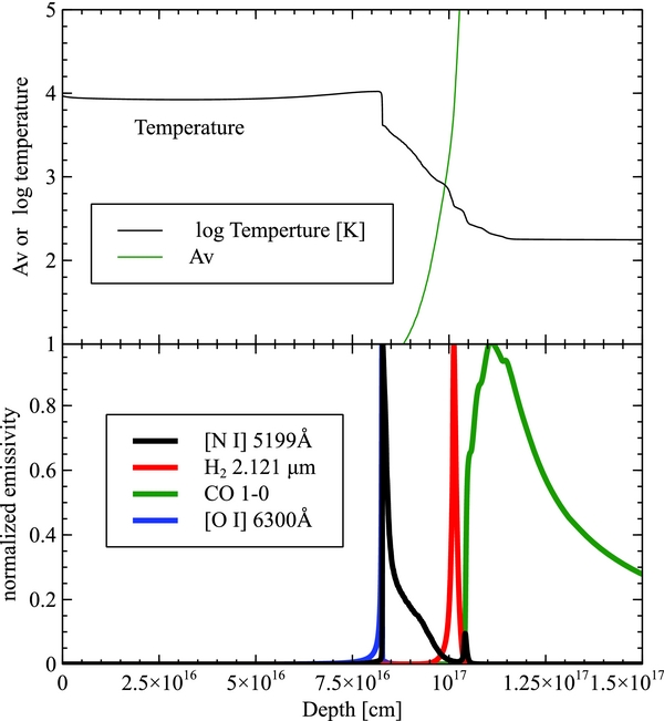
Figure 3. Temperature, extinction, and emissivity of several important emission lines are shown as a function of depth into the H+ layer. The upper panel shows the log of the gas kinetic temperature and the visual extinction AV, with the values of both indicated on the left axis. The lower panel shows the normalized emissivity for several important lines. This is the volume emissivity (erg cm−3 s−1) divided by the peak emissivity for each line to place them on the same scale.
Download figure:
Standard image High-resolution imageThe lower panel of Figure 3 shows the volume emissivity of the λ5199+ lines along this ray. For reference the lower panel also shows the emissivity of some well-observed H2, CO, and [O i] lines. We see that both [O i] and [N i] lines form near the H+–H0 ionization front, while the H2 and CO lines form near the H0–H2 dissociation front.
The H2 line is mainly formed by continuum fluorescent excitation for a PDR near an H ii region (Tielens & Hollenbach 1985). This formation processes is very similar to that forming the [N i] lines. The H2 and [N i] lines form at either edge of the PDR due to a combination of abundance and FUV line optical depth effects.
Figure 4 shows the volume emissivity of the [N i] line as a function of gas kinetic temperature. This is a convenient way to visualize the rapid changes in emissivity that occur near the H+–H0 ionization front, where both emissivity and temperature change rapidly. This does not indicate the total contribution of various processes to the observed line since the surface brightness is the integral of the emissivity over the emitting volume. The size of each volume element changes dramatically as the conditions change.

Figure 4. Volume emissivity of [N i] λ5199+ vs. gas kinetic temperature. This is a different view of the data in Figure 3. The total emissivity and the contributions from collisions, continuum pumping, and the chemical dissociation processes described in Appendix A are shown.
Download figure:
Standard image High-resolution imageThe peak emissivity occurs at a gas kinetic temperature of ∼4000 K, with contributions from continuum pumping and collisions. The emissivity increases as the temperature decreases due to the increasing N0 abundance in cooler regions. Continuum pumping increases with increasing N0 abundance. The emissivity decreases at lower temperatures due to increasing optical depths in the FUV lines. The rise in emissivity at temperatures ∼300 K is due to formation by molecular dissociation, using the estimates outlined in Appendix A.4.
3.2. The Effects of Non-thermal Broadening
Given these assumptions the only free parameter is the turbulent contribution to the line width. Figure 5 shows the predicted [N i] 5199+/Hβ intensity ratio as function of the turbulence. We have determined the broadening of the [N i] lines from spectra made with the HIRES spectrograph as part of a program studying mass loss from proplyds in the Huygens Region (Henney & O'Dell 1999). In the proplyd-free portions of these long-slit spectra, the average observed FWHM was 13.65 ± 1.91 km s−1. The instrumental FWHM of the comparison lines was 8.28 ± 0.40 km s−1. If the [N i] emission arises from the region with T = 1000–3000 K, then the thermal component of the broadening would be 2–3 km s−1. After quadratic subtraction of the instrumental and thermal widths from the observed FWHM, there is a residual non-thermal broadening component of 10.6 ± 1.9 km s−1. The four proplyds in the sample (150–353, 170–337, 177–341, 182–413) have an average distance from θ1 Ori C of 0.56 ± 0 29. After examination of panel (A) of Figure 1, we see that the expected ratio I([N i])/I(Hβ) would be 0.0034 ± 0.0007. These values are indicated in Figure 5 for comparison with the predictions of our model. The line width is given as an upper limit, since the observed emission profile will in general include contributions from macroscopic and microscopic broadening processes (see discussion in Appendix C) whereas only the latter will contribute to the pumping efficiency.

Figure 5. Surface brightness of the [N i] line relative to Hβ as a function of the FWHM of the non-thermal line broadening component in the [N i] formation region. The observed ratio is indicated along with error bars that represent the scatter in the ratio. The observed FWHM is indicated and is really an upper limit to the microturbulent broadening, as discussed in Appendix B.
Download figure:
Standard image High-resolution imageIn Appendix A, we show that in the fluorescent scenario the strength of the [N i] emission lines with respect to Hβ is close to linearly proportional to the degree of line broadening in the region in which the lines are pumped. In order to reproduce the observed brightness, our model requires an FWHM for the broadening (assuming a Gaussian line profile) of ≃ 10 km s−1. If this broadening were to be thermal, then a temperature of >10, 000 K in the pumping region would be required, which is much larger than the ≈2000 K predicted by our Cloudy model. Instead, it is likely that the majority of the broadening is non-thermal in nature. Significant non-thermal line widths have been reported in the spectra of Orion Nebula emission lines (O'Dell 2001; O'Dell et al. 2003; García-Díaz et al. 2008). The nature of the processes producing this broadening is not known, but it must be important as its magnitude indicates that as much energy is contained there as is contained in the components explained by basic photoionization physics.
4. DISCUSSION
4.1. Spatial Variation of Intensity Ratios
In Section 3, we established a model of an essentially substellar point in the Orion Nebula that adequately explains the observed I([N i])/I(Hβ) line ratios. However, we see in Figure 1(A) that this ratio varies across the Huygens Region and its near vicinity, rising monotonically with increasing distance from θ1 Ori C. A similar increase is seen for the line ratios in M43 with increasing distance from NU Ori. On the other hand, Figure 6 shows that the corrected equivalent width of the [N i] lines is essentially constant at 2 ± 1 Å and shows no detectable variation either within M42, nor between M42 and M43. Since the PDR is optically thick to the irradiating stellar continuum, its visual scattered light is a measure of the FUV continuum that pumps the upper states of 5199+. The quantitative relation is determined by the scattering properties of the grains. These are elaborated in Appendix B.

Figure 6. Equivalent width of the [N i] 5199+ vs. equivalent width of Hβ.
Download figure:
Standard image High-resolution imageAppendix B shows that the line intensity ratios and equivalent widths can be expressed in terms of the ratios of "scattering" efficiencies (albedos) and the ratios of the stellar continuum luminosities in different wavelength bands. The pumping contribution to 5199+ depends on the intensity of the SED around 1000 Å while the intensity of Hβ, which forms by recombination, is proportional to the continuum intensity at hydrogen-ionizing energies. These are denoted by FUV and EUV in Table 2. In the simplest case we expect the 5199+/Hβ intensity ratio to scale with FUV/EUV, while the 5199+ equivalent width should scale with FUV/visual.
Table 2. Spectral Energy Distributions over Selected Wavelength Intervals
| Group | SED Ratio | |||
|---|---|---|---|---|
| FUV/Visual | EUV/Visual | FUV/EUV | EW(Hβ, Int) (Å) | |
| M42 inner | 20.34 | 7.36 | 2.76 | 380 |
| M42 outer | 18.18 | 4.39 | 4.14 | 213 |
| M43 | 19.02 | 1.40 | 13.62 | 81 |
| Ring Nebula | 76.33 | 192.24 | 0.40 | |
| Crab Nebula | 1.10 | 1.12 | 0.99 | |
Notes. Columns 2–4 show the ratio of 〈λLλ〉 between different wavelength bands: EUV = 507–912 Å; FUV = 950–1200 Å; visual = 4800–4900 Å. Column 5 shows the "intrinsic" equivalent width LHβ/Lλ of the stellar population, where the continuum luminosity Lλ is evaluated adjacent to the Hβ line and line luminosity LHβ is calculated as described in the text. Results are shown for the three stellar groupings of Table 1, using atmosphere models from Lanz & Hubeny (2003, 2007). The Ring and Crab Nebulae are considered in Section 4.5.
Download table as: ASCIITypeset image
4.2. The Importance of the FUV/EUV Ratio
Table 2 lists the ratios of the average value of the SED λLλ, calculated for the visual, FUV, and ionizing EUV bands, and for three different OB stellar populations characteristic of the inner Orion Nebula (Trapezium region), the outer Orion Nebula, and M43 (we will consider the Crab and Ring Nebulae, objects very different from Orion and with strong [N i] emission, in Section 4.5 below). It can be seen from the table that the FUV/visual luminosity ratio is approximately constant between the three stellar populations in Orion (variation <10%), which arises because the spectral shape in all cases approximately follows the Rayleigh–Jeans behavior of Lλ ∼ λ−2. On the other hand, the relative strength of the EUV band with respect to the FUV and optical bands shows significant variation, being roughly five times greater for the Trapezium stars than for the exciting star of M43. We suggest that it is the presence or otherwise of variations in the broadband illuminating spectrum that is the principal determinant of the observed spatial variations in intensity ratios.
4.3. The Importance of the Constant Equivalent Width
The observed constant value of EW([N i], Corr), coupled with the lack of variation in  implies (Equation (B5)) that the ratio of [N i] albedo to dust-scattering albedo is also constant within and between the nebulae:
  . The Cloudy model of Section 3 implies that
  for a non-thermal broadening of 5 km s−1 if the illumination and viewing angles are both close to face-on (see Figure 11(b)). The dust-scattering effective albedo is therefore constrained to be 0.5 ± 0.3, which is consistent with the expectations for back-scattering from the background molecular cloud (see Appendix B.2.3 and Figure 12) so long as the single-scattering albedo is relatively high.
4.4. Variation in the I([N i])/I(Hβ) Ratio
The ratio I([N i])/I(Hβ) (Figure 1(A)) increases by roughly a factor of three between the inner and outer regions of M42 and by a factor of 4–8 between M42 and M43. The different values of  for the stellar populations (Table 2) can fully explain the difference between M42 and M43 but can only account for half of the variation within M42 and cannot explain any of the variation within M43 (where the single dominant star means that the illuminating spectrum should be constant). This implies that a small systematic increase with radius within each nebula of the ratio of albedos
  may also play a role. The analysis of Appendix B.2.1 shows that ϖHβ ≃ 0.1 when the illumination and viewing angles are face-on, which, combined with the above value of
  and using Equation (B3), implies I([N i])/I(Hβ) ≃ 0.03 for illumination by the Trapezium spectrum, as is observed for the innermost regions of M42. Inspection of Figure 11 shows that, as long as the plane-parallel approximation is valid, variations in the viewing angle cannot account for the inferred increase in
  with radius since the two albedos depend on angle in a similar way, except for close to edge-on orientations where
  is predicted to decrease. However, as discussed in Appendix B.4, a finite curvature of the scattering layer has the effect of limiting the limb brightening for edge-on viewing angles, and this effect is much greater for Hβ, where the scattering layer is much thicker than for [N i]. This effect may explain the increase in
  if the average viewing angle became increasingly edge-on in the outskirts of the nebula (see Appendix B.3 for further discussion). An alternative explanation could be an increase with radius of the turbulent broadening within the fluorescent [N i] layer, but there is no independent evidence for such an increase.
4.5. The I([N i])/I(Hβ) Ratio in Other Classes of Nebulae
The original motivation for this work was to calibrate models of the formation of [N i] lines in the relatively quiescent Orion environment, as a step toward understanding what these lines indicate in the more exotic environments where they are unusually strong. Although continuum fluorescent excitation does account for the [N i] lines in Orion, the process cannot produce the stronger [N i] emission seen in planetary nebulae or the Crab supernova remnant.
The last two rows of Table 2 show the continuum intensity ratios produced by the SEDs of the Ring Nebula (a T = 1.2 × 10⁵ K Rauch stellar atmosphere; O'Dell et al. 2007) and the Crab Nebula (Davidson & Fesen 1985). The [N i]/Hβ intensity ratio scales with the FUV/EUV continuum ratio. Table 2 shows that this ratio is 7 and three times smaller for the Ring and Crab Nebulae than in Orion. Accordingly, the continuum fluorescent excitation contribution to the [N i]/Hβ intensity ratio produced by fluorescence will be of order I([N i])/I(Hβ) ∼ 10−3. The observed line ratio is several orders of magnitude larger, showing that other processes must be at work. Thermal excitation by warm gas, perhaps produced by penetrating energetic photons or ionizing particles, seems to be needed. High-resolution observations of the lines given in Figure 9 could test whether thermal processes do account for the observed spectrum.
5. CONCLUSIONS
There are multiple conclusions that can be drawn from the work reported upon in this paper. Some are positive, in the sense that we find quantitative explanations for detailed observations of the Orion Nebula, while some are negative, in the sense that we demonstrate that the FUV pumping mechanism cannot be the dominant process in objects like the planetary nebula the Ring Nebula and supernova remnants like the Crab Nebula. The specific conclusions are summarized below.
- 1.The [N i] doublet is produced not by collisional excitation out of the lower-lying ground state of neutral nitrogen. Rather, it is the result of FUV continuum radiation being absorbed and populating a higher electronic state which then populates the upper states of the [N i] doublet by cascade.
- 2.The process operates in the thin transition boundary of the PDR that is close to the overlying ionization front.
- 3.This process means that one cannot use the relative strength of the two members of the [N i] doublet as density indicators.
- 4.In order for this mechanism to produce the intensity of the [N i] emission seen in the Huygens Region of the Orion Nebula there must be a non-thermal component to the broadening of the FUV absorption line that drives the process, with FWHM of approximately 5 km s−1 (see Figure 5). We argue in Appendix C that the origin of this broadening cannot be the same as the transonic turbulence that is believed to be responsible for broadening the optical emission lines in the H ii region because the latter operates at too large a scale to affect the radiative transfer in the thin pumping layer. Instead, we suggest that small-scale thermal instabilities may be responsible.
- 5.The constant value of the equivalent width of the [N i] doublet with respect to the underlying scattered light continuum can be interpreted as the PDR being optically thick to scattered starlight and a combination of reasonable assumptions about the scattering properties of the solid particles in the PDR and the orientation of the PDR.
- 6.The efficacy of this pumping process is critically dependent upon the ratio of FUV/EUV radiation from the illuminating sources. We show that the stars associated with the Orion Nebula and the independent low-ionization H ii region M43 explain the different amounts of [N i] excess emission in these very different objects.
- 7.The FUV/EUV ratio for a bright planetary nebula (the Ring Nebula) and the well observed Crab Nebula supernova remnant indicate that the FUV pumping mechanism that explains the Orion Nebula and M 43 is not the source of the excess [N i] emission in those objects.
We thank the referee for a careful review of the manuscript. G.J.F. acknowledges support by NSF (0908877; 1108928; and 1109061), NASA (07-ATFP07-0124, 10-ATP10-0053, and 10-ADAP10-0073), JPL (RSA No 1430426), and STScI (HST-AR-12125.01, GO-12560, and HST-GO-12309). W.J.H. acknowledges financial support from DGAPA-UNAM through grant PAPIIT IN102012. C.R.O. was supported in part by STScI grant GO-11232. P.v.H. acknowledges support from the Belgian Science Policy Office through the ESA Prodex program. This research used data from the Atomic Line List (http://www.pa.uky.edu/~peter/atomic).
APPENDIX A: THE N i EMISSION MODEL
Here we describe recent improvements in the treatment of N i emission in the spectral simulation code Cloudy. Our model includes many emission processes because it is intended to be general, and applicable to other environments.
A.1. The Atomic Model
In order to optimize the speed of the model, we have chosen to model the N i atom using a five-level atom for the metastable levels. The fluorescence processes discussed in this paper (as well as the recombination pumping) are added as rates populating the various excited metastable levels. The level energies were obtained from Moore (1975) and the lowest five levels are listed in Table 3 and shown in Figure 7. An additional 10 FUV lines can absorb photons in the 951–1161 Å range. These lines drive the fluorescence process and will be discussed in more detail below.
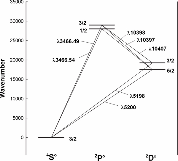
Figure 7. Lowest five levels of the N i model. The 5198, 5200 Å pair of lines are denoted by λ5199+ in the text. A fourth line of the IR multiplet, 2P1/2–2D3/2 at 10408 Å, is not shown for clarify.
Download figure:
Standard image High-resolution imageTable 3. [N i] Energy Levels
| Configuration | Term | J | Energy (cm−1) |
|---|---|---|---|
| 2s22p3 | 4So | 3/2 | 0.000 |
| 2s22p3 | 2Do | 5/2 | 19 224.464 |
| 3/2 | 19 233.177 | ||
| 2s22p3 | 2Po | 1/2 | 28 838.920 |
| 3/2 | 28 839.306 |
Download table as: ASCIITypeset image
Transition probabilities have been computed by Butler & Zeippen (1984), Godefroid & Fischer (1984), Hibbert et al. (1991), Tachiev & Froese Fischer (2002), and Froese Fischer & Tachiev (2004).
Table 4 compares the Butler & Zeippen (1984) and Godefroid & Fischer (1984) rates for the forbidden transitions, referred to as the "1984" rates, with the more recent calculation of Froese Fischer & Tachiev (2004), referred to as the "2004" rates. The latter rates are used. Hibbert et al. (1991) do not give transition probabilities for the forbidden transitions.
Table 4. [N i] Transition Probabilities
| Air Wavelength | Transition | 1984 | 2004 |
|---|---|---|---|
| 5200.3 | 2Do5/2 → 4So3/2 | 5.77(−6) | 7.57(−6) |
| 5197.9 | 2Do3/2 → 4So3/2 | 2.26(−5) | 2.03(−5) |
| 3466.543 | 2Po1/2 → 4So3/2 | 2.52(−3) | 2.61(−3) |
| 3466.497 | 2Po3/2 → 4So3/2 | 6.21(−3) | 6.50(−3) |
| 10398.2 | 2Po1/2 → 2Do5/2 | 3.03(−2) | 3.45(−2) |
| 10397.7 | 2Po3/2 → 2Do5/2 | 5.39(−2) | 6.14(−2) |
| 10407.6 | 2Po1/2 → 2Do3/2 | 4.63(−2) | 5.27(−2) |
| 10407.2 | 2Po3/2 → 2Do3/2 | 2.44(−2) | 2.75(−2) |
Download table as: ASCIITypeset image
The electron collision rates for [N i] have been the subject of a number of studies. Berrington et al. (1975) computed electron collision cross sections which Dopita et al. (1976) converted into collision strengths. These were later summarized by Berrington & Burke (1981). Dopita et al. (1976) found some discrepancies with existing observations and speculated that the disagreement was due to uncertainties in the collision strengths. Tayal (2000) presented close-coupling calculation of the effective collision strengths while Tayal (2006) redid the calculation with significantly different results.
Table 5 gives the history of these electron collision strengths. The 4So − 2Do collision strength affects the intensity of the collisionally excited contribution to the [N i] λ5199+ lines, while the 2Do3/2 − 2D1/2o collision strength affects the density diagnostic. The Berrington & Burke (1981) and Tayal (2006) results are in reasonable agreement suggesting that the theoretical calculations have converged onto a stable value.
Table 5. History of [N i] Collision Strengths at 104 K
| Reference | 4So − 2Do | 2Do3/2 − 2D1/2o |
|---|---|---|
| Berrington & Burke 1981 | 0.48 | 0.27 |
| Tayal 2000 | 0.044 | 3.24 |
| Tayal 2006 | 0.561 | 0.257 |
Download table as: ASCIITypeset image
We know of no rates for collisions with hydrogen atoms. This should be included since we expect that [N i] may form in shallow regions of the PDR, where n(H0) ≫ ne. Cloudy does include a general correction for H0 collisions based on the ne rate. The effective electron density, with this correction, is ne + 1.7 × 10⁻⁴n(H0) based on the discussion by Drawin (1969).
Cloudy includes many other line formation processes in addition to thermal collisional impact excitation (Ferland & Rees 1988). Continuum pumping of the FUV lines around 1000 Å will be very important. We treat this as described in Ferland (1992) and Shaw et al. (2005). Fluorescent excitation is mainly produced by stellar FUV photons. Pumping will be efficient until the N i lines become optically thick At this point they will have absorbed stellar photons over the Doppler width of the line. Below we explore how the pumping efficiency depends on the turbulent contributor to the line width. Other opacity sources will affect the strength of the pumped contributor to N i by removing FUV photons before they are absorbed by N i. The two most important opacity sources are extinction of the stellar radiation field by grains within the H ii region and PDR, and shielding by the forest of overlapping H2 lines in deeper parts of the PDR. These processes are all included self-consistently in our calculations.
A.2. The Fluorescence Mechanism
In strict LS coupling, transitions that change the total spin of the atom (called intercombination transitions) are forbidden and FUV pumping out of the quartet ground term could not eventually populate the doublet excited terms that produce the observed lines. However, deviations from strict LS coupling make it possible that a significant fraction of excitations by FUV photons will eventually populate the excited doublets. There are two possible routes: either direct excitation by an intercombination line from the ground state or indirect excitation by a resonance line followed by de-excitation through an intercombination line. In the case of N i both routes contribute. A complete list of the driving lines can be found in Table 6. For each of the driving lines we calculate a two-level atom giving us the excitation rate for each of these transitions. We also calculated branching ratios for the cascade down from each of the upper levels. In these calculations, we exclude the transition straight back to the ground state as this does not destroy the photon. Instead it can be absorbed over and over again until finally a different cascade from the upper level occurs (this neglects background opacities which will be discussed further down). Intercombination lines from the doublet system back to the quartet system are included in the cascade, but not tracked any further after that. This implies that routes quartet → doublet → quartet → doublet are not included in the pumping rates. We expect the error introduced by this approximation to be negligible. The branching ratios were calculated using transition probabilities from Froese Fischer & Tachiev (2004). By combining all different routes in the cascade we could calculate a probability that an excitation of a given driving line would result in populating any of the metastable levels. The results of these calculations are shown in Table 7. The list of intercombination lines populating the doublet metastable levels after an excitation in the Ind1 driving line is given in Table 8.
Table 6. The Lines Driving the N i Fluorescence
| Label | Upper Level | Ek (cm−1) | Aki (s−1) | a | b |
|---|---|---|---|---|---|
| Ind1 | 2s22p2 (3P) 3d4P5/2 | 104 825.110 | 1.62(8) | −11.3423 | 0.8379 |
| Dir1 | 2s22p2 (3P) 3d2F5/2 | 104 810.360 | 1.95(7) | −12.3982 | 0.7458 |
| Dir2 | 2s22p2 (3P) 3d2D5/2 | 105 143.710 | 8.29(5) | −9.4523 | 0.3865 |
| Dir3 | 2s22p2 (3P) 3d2P3/2 | 104 615.470 | 4.29(5) | −12.5580 | 0.7330 |
| Dir4 | 2s22p2 (3P) 4s2P3/2 | 104 221.630 | 3.75(5) | −10.8813 | 0.6853 |
| Dir5 | 2s22p2 (3P) 3d2P1/2 | 104 654.030 | 2.63(5) | −13.6532 | 0.7712 |
| Dir6 | 2s22p2 (3P) 3d2D3/2 | 105 119.880 | 1.71(5) | −9.9035 | 0.3919 |
| Dir7 | 2s22p2 (3P) 4s2P1/2 | 104 144.820 | 1.69(5) | −11.4470 | 0.6734 |
| Dir8 | 2s22p2 (3P) 3s2P3/2 | 86 220.510 | 4.94(4) | −5.4776 | 0.1789 |
| Dir9 | 2s22p2 (3P) 3s2P1/2 | 86 137.350 | 2.72(4) | −6.3304 | 0.1966 |
Notes. For each of the lines, the lower level is the ground state of N i. The level energies are taken from Moore (1975) and the transition probabilities from Froese Fischer & Tachiev (2004). The effective collision strength is given by the fitting formula ϒ = exp (a + bmin [ln T, 10.82]) where the original data were obtained from Tayal (2006).
Download table as: ASCIITypeset image
Table 7. Probability Ppump of Populating a Metastable Level after an Excitation in Each of the Driving Lines
| Level | Ind1 | Dir1 | Dir2 | Dir3 | Dir4 | Dir5 | Dir6 | Dir7 | Dir8 | Dir9 |
|---|---|---|---|---|---|---|---|---|---|---|
| 2Do5/2 | 0.0417 | 0.0468 | 0.3408 | 0.2328 | 0.7937 | 0.1338 | 0.0623 | 0.0238 | 0.6615 | 0.0000 |
| 2Do3/2 | 0.3441 | 0.8621 | 0.0233 | 0.0895 | 0.1068 | 0.1644 | 0.2908 | 0.8397 | 0.0694 | 0.7369 |
| 2Po1/2 | 0.0113 | 0.0239 | 0.0090 | 0.1617 | 0.0167 | 0.4404 | 0.4881 | 0.0876 | 0.0450 | 0.1777 |
| 2Po3/2 | 0.0112 | 0.0265 | 0.6253 | 0.5108 | 0.0824 | 0.2588 | 0.1569 | 0.0484 | 0.2240 | 0.0854 |
Download table as: ASCIITypeset image
Table 8. The List of Intercombination Lines that Can Occur after an Excitation in the Ind1 Driving Line
| Lower Level | Ei (cm−1) | Aki (s−1) |
|---|---|---|
| 2s22p3 2D3/2 | 19 233.177 | 1.24(7) |
| 2s22p2 (3P) 3p2D3/2 | 96 787.680 | 2.92(6) |
| 2s22p3 2D5/2 | 19 224.464 | 1.30(6) |
| 2s22p2 (3P) 3p2D5/2 | 96 864.050 | 2.16(5) |
| 2s22p3 2P3/2 | 28 839.306 | 1.06(5) |
| 2s22p2 (3P) 3p2P3/2 | 97 805.840 | 9.87(3) |
Notes. For each line the upper level is 2s22p2 (3P) 3d4P5/2. The level energies are taken from Moore (1975) and the transition probabilities from Froese Fischer & Tachiev (2004).
Download table as: ASCIITypeset image
In the previous discussion, we mentioned that transitions in any of the driving lines straight back to the ground level were not counted because these photons would simply be re-absorbed until a different cascade occurs. This assumption is not entirely correct as there is a finite probability Pdest that the photon is destroyed before it can be absorbed again (e.g., due to background opacities such as the grain opacity or bound-free opacity of elements with sufficiently low-ionization potentials). Additionally, there is a probability Pesc that the photon escapes from the cloud before it can be absorbed again. In order to account for these processes, we modify the excitation rate j2 in s−1 obtained from the two-level atom as follows:
where β is a constant that gives the fraction of excitations in a driving line that is followed directly by a de-excitation back to the ground level. For Ind1 β = 0.7955 and for Dir1 β = 0.1384. For all other driving lines β < 0.01 and is assumed to be zero. Given this formula we can the write the total pump rate for each of the metastable levels as
where the summation runs over all the driving lines and the constants P ipump are given in Table 7 for each of the metastable levels and driving lines.
For completeness we should also mention that pumping of the metastable states through recombination from N+ is also included in our modeling. We use the formulae given in Pequignot et al. (1991). These only give the rates to the full 2D and 2P metastable terms. In our modeling we split up these rates for each level according to statistical weight. This pumping mechanism will of course only be effective inside the ionized region as nitrogen has a slightly higher ionization potential than hydrogen.
From the data in Table 6 it is clear that all driving lines have wavelengths longward of the Lyman limit. This implies that the fluorescence mechanism is effective beyond the ionization front in the PDR. Since the temperature in the PDR is generally too low to collisionally excite the metastable doublet states, fluorescence can even become the dominant excitation mechanism for the forbidden N i lines in the PDR. It should also be noted that even very weak direct excitation lines can have a significant contribution to the fluorescence mechanism. If the PDR has sufficient column density, then all driving photons will eventually be absorbed. A low transition probability in the driving line only means that the effect is spread over a larger area.
The fluorescence mechanism will produce permitted N i emission lines that are observable in deep spectra. The cascade routes that populate the metastable levels will produce lines in the doublet system with wavelengths ranging between 8567 Å and 5.382 μm, as well as UV lines that cannot be observed from the ground. The shortest wavelength lines will tend to be the strongest since they come from the lowest levels where there are only a few alternative routes the cascade can take. In the ionized region these lines can also be produced by recombination from N+ → N0, but in the PDR these lines can only be produced by the fluorescence mechanism described here. So if these lines are observed in the PDR, it is conclusive proof for continuum pumping of the [N i] lines. In Table 9 we list all optical cascade lines with wavelengths shorter than 1 μm and in Table 10 we list the branching probabilities for each of the driving lines. Excitations by the Dir8 and Dir9 driving lines only produce UV cascade lines and are therefore not included in Table 10. Each driving line has its own characteristic spectrum. The relative strength of the contribution for each driving line depends on the incident spectrum, the optical depth in each of the driving lines, and the escape and destruction probability for the Ind1 and Dir1 driving lines. So no generic prediction for the spectrum can be made. However, a straight average indicates that the λλ9387, 9029, 9060, and 8629 lines will be the strongest, with the λ9387 line having about 1.8% of the flux of the λ5199+ doublet. It should be noted that the cascade lines shown in Table 9 are not predicted by Cloudy.
Table 9. The List of Permitted Lines in the Doublet System That Can be Excited by the Fluorescence Mechanism Described Here
| λair | Transition | Aki (s−1) |
|---|---|---|
| 8567.735 | 2s22p2 (3P) 3p2P°3/2 → 2s22p2 (3P) 3s2P1/2 | 4.87(6) |
| 8594.000 | 2s22p2 (3P) 3p2P°1/2 → 2s22p2 (3P) 3s2P1/2 | 2.10(7) |
| 8629.235 | 2s22p2 (3P) 3p2P°3/2 → 2s22p2 (3P) 3s2P3/2 | 2.68(7) |
| 8655.878 | 2s22p2 (3P) 3p2P°1/2 → 2s22p2 (3P) 3s2P3/2 | 1.08(7) |
| 9028.922 | 2s22p2 (3P) 3d2P1/2 → 2s22p2 (3P) 3p2S°1/2 | 3.20(7) |
| 9060.475 | 2s22p2 (3P) 3d2P3/2 → 2s22p2 (3P) 3p2S°1/2 | 3.21(7) |
| 9386.805 | 2s22p2 (3P) 3p2D°3/2 → 2s22p2 (3P) 3s2P1/2 | 2.14(7) |
| 9392.793 | 2s22p2 (3P) 3p2D°5/2 → 2s22p2 (3P) 3s2P3/2 | 2.52(7) |
| 9395.848 | 2s22p2 (3P) 4s2P3/2 → 2s22p2 (3P) 3p2S°1/2 | 1.81(4) |
| 9460.676 | 2s22p2 (3P) 3p2D°3/2 → 2s22p2 (3P) 3s2P3/2 | 3.74(6) |
| 9464.169 | 2s22p2 (3P) 4s2P1/2 → 2s22p2 (3P) 3p2S°1/2 | 3.50(5) |
Notes. Only lines with wavelengths between 8567 Å and 1 μm are listed. The transition probabilities were taken from Froese Fischer & Tachiev (2004).
Download table as: ASCIITypeset image
Table 10. Branching Probabilities of the Cascade Lines for Each of the Driving Lines
| λair | Ind1 | Dir1 | Dir2 | Dir3 | Dir4 | Dir5 | Dir6 | Dir7 |
|---|---|---|---|---|---|---|---|---|
| 8567.735 | 0.0000 | 0.0001 | 0.0158 | 0.0016 | 0.0085 | 0.0015 | 0.0035 | 0.0025 |
| 8594.000 | 0.0000 | 0.0000 | 0.0000 | 0.0031 | 0.0082 | 0.0129 | 0.0549 | 0.0229 |
| 8629.235 | 0.0002 | 0.0008 | 0.0868 | 0.0086 | 0.0469 | 0.0082 | 0.0190 | 0.0135 |
| 8655.878 | 0.0000 | 0.0000 | 0.0000 | 0.0016 | 0.0041 | 0.0065 | 0.0275 | 0.0115 |
| 9028.922 | 0.0000 | 0.0000 | 0.0000 | 0.0000 | 0.0000 | 0.2840 | 0.0000 | 0.0000 |
| 9060.475 | 0.0000 | 0.0000 | 0.0000 | 0.2546 | 0.0000 | 0.0000 | 0.0000 | 0.0000 |
| 9386.805 | 0.0597 | 0.1270 | 0.0004 | 0.0045 | 0.0040 | 0.0196 | 0.0343 | 0.0532 |
| 9392.793 | 0.0052 | 0.0058 | 0.0487 | 0.0256 | 0.0534 | 0.0000 | 0.0059 | 0.0000 |
| 9395.848 | 0.0000 | 0.0000 | 0.0000 | 0.0000 | 0.0002 | 0.0000 | 0.0000 | 0.0000 |
| 9460.676 | 0.0104 | 0.0222 | 0.0001 | 0.0008 | 0.0007 | 0.0034 | 0.0060 | 0.0093 |
| 9464.169 | 0.0000 | 0.0000 | 0.0000 | 0.0000 | 0.0000 | 0.0000 | 0.0000 | 0.0027 |
Note. Excitations by the Dir8 and Dir9 driving lines do not produce any optical cascade lines.
Download table as: ASCIITypeset image
At this point we should discuss the accuracy of the transition probabilities of the intercombination lines. Accurate values for such lines are hard to obtain since they are quite sensitive to the details of the calculation. However, for direct excitation lines, accurate values for the transition probability are not crucial. Using the argument from the previous paragraph it becomes clear that an error in the transition probability would only imply that the absorption of the driving photons would happen over a smaller or larger area, but the total amount of pumping would remain the same when integrated over the entire PDR. This of course assumes that the PDR is optically thick. If that is not the case, then an error in the transition probability would alter the escape probability of the driving line. In such circumstances accurate transition probabilities are needed. For indirect excitation lines, accurate transition probabilities are always needed (even when the PDR is optically thick) since the intercombination line has to compete with stronger, fully allowed transitions in the cascade down from the upper level of the driving line. However, this problem is mitigated by the fact that there is only one indirect driving line versus nine direct driving lines. So, an error in this component would only have a limited effect on the total pumping. In Table 11, we compare the transition probabilities of the lines involved in the cascade down from the indirect excitation using data from Hibbert et al. (1991, length form) and Froese Fischer & Tachiev (2004). It is apparent that discrepancies up to 1 dex and more can occur, indicating the difficulty in calculating these data.
Table 11. Comparison of the Transition Probability for Various Intercombination Lines Used in Our Model
| Lower Level | 1991 | 2004 |
|---|---|---|
| 2s22p3 2D3/2 | 9.08(5) | 1.24(7) |
| 2s22p2 (3P) 3p2D3/2 | 3.43(5) | 2.92(6) |
| 2s22p3 2D5/2 | 1.02(6) | 1.30(6) |
| 2s22p2 (3P) 3p2D5/2 | 6.48(4) | 2.16(5) |
| 2s22p3 2P3/2 | 1.04(6) | 1.06(5) |
| 2s22p2 (3P) 3p2P3/2 | 5.67(4) | 9.87(3) |
Notes. For each line the upper level is 2s22p2 (3P) 3d4P5/2. The transition probabilities (units s−1) are taken from Hibbert et al. (1991, labeled "1991") and Froese Fischer & Tachiev (2004, labeled "2004"). The latter were used in our model.
Download table as: ASCIITypeset image
A.3. Density–Temperature Diagnostics in the Collisional Excitation Case
If the lines were collisionally excited then the electron density could be determined from the ratios of the intensities of two lines of the same ion, emitted by different levels with nearly the same excitation energy (AGN3). Temperature is indicated by emission from levels with different excitation energies. Together, the gas pressure could be directly measured. This can test whether the lines are thermally excited, and is useful for reference by future studies which will look into the formation of [N i] lines in planetary nebulae, the Crab Nebula, and cool-core cluster filaments.
We show several emission line diagnostics for the collisionally dominated case, using our updated atomic data and model atom. Line pairs such as the ratio of lines of [N i]

indicate the electron density in gaseous nebulae, as shown by Seaton & Osterbrock (1957) and Saraph & Seaton (1970) for [O ii]. Note that the energy order of the J levels within the 2D term depends on both the charge and electronic configuration. The line ratio is defined so that it decreases as density increases.
Every collisional excitation is followed by the emission of a photon in the low-density limit. Since the relative excitation rates of the 2D5/2 and 2D3/2 levels are proportional to their collision strengths, the ratio is
This is valid when kT ≫ δ , where δ is the difference in energies of the upper levels. This holds for all temperatures where the optical lines emit due to the small energy difference of the upper levels. In the high-density limit collisional processes dominate and set up a Boltzmann level population distribution. The relative populations of the 2D5/2 and 2D3/2 levels are in the ratio of their statistical weights, and the relative intensities of the two lines are in the ratio
The line ratio varies between these intensity limits as the density varies. The critical density, the density where the collisional and radiative de-excitation rates are equal, is ncrit ∼ 103 cm−3 at ∼104 K.
Figure 8 compares the [N i] Rn with the more commonly used [O ii], [S ii], and [Cl iii] density indicators using data from B2000. The [O ii] collision strengths computed by Kisielius et al. (2009) were used. The behavior of these curves is qualitatively similar, going to the ratio of statistical weights at low densities and a ratio that depends on the radiative transition probabilities at high densities.
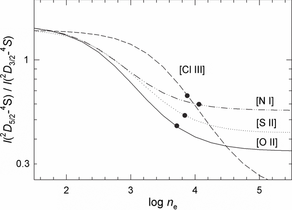
Figure 8. [N i] and three of the commonly used density indicators present in optical spectra. The points are from B2000.
Download figure:
Standard image High-resolution imageThe gas kinetic temperature can be determined from ratios of intensities from two levels with considerably different excitation energies. For [N i] we have the ratio
These density–temperature indicators can be combined to form a unified diagnostic diagram, as has long been done for [O iii] (AGN3 Figure 5.12). Figure 9 shows calculated curves of the values of the two [N i] intensity ratios for various values of T and ne.

Figure 9. Derived density and temperature, in units of log ne (cm−3) and 104 K respectively, as deduced from line intensity ratios from the model [N i] atom.
Download figure:
Standard image High-resolution imageWe used the line intensities measured in bright central regions (B2000; Esteban et al. 2004, hereafter E2004) to estimate ne and T. B2000 presented high-resolution spectrophotometric observations of the Orion Nebula in the 3500–7060 Å range. Their slit position was 37'' west of θ1 Ori C. This is close to the position modeled by Baldwin et al. (1991). E2004 covered the 3100–10400 Å range. Their slit was oriented east–west and centered at 15 arcsec south and 10 arcsec west of θ1 Ori C.
Rn was 0.60 ± 0.02 for the average of the blue and red spectra in B2000 and 0.59 for E2004. This is plotted in both Figures 8 and 9. The results are surprising—the electron density indicated by the [N i] lines, which should form in partially ionized gas giving lower electron densities, is 0.2–0.4 dex larger than densities indicated by lines which form in highly ionized regions.
It is not now possible to measure the temperature using the λ3467+ line. We know of no detection of this line in the Orion environment. However Esteban et al. (1999) reported the upper limit of I(3467+)/I(Hβ) < 10−3 from the data presented by Osterbrock et al. (1992). This corresponds to λ3467+/λ5199+ < 0.22.
These values of the line ratios are shown in Figure 9. The temperature limit indicated by the line is consistent with formation in a photoionized environment. The high density would be surprising if true. Actually this can be taken as independent evidence that the lines do not form by collisional excitation.
A.4. Dissociation of Nitrogen-bearing Molecules
Störzer & Hollenbach (2000) show that significant optical [O i] emission can result from dissociation of oxygen-bearing molecules. Could an analogous process contribute to the [N i] emission we observe in Orion?
Störzer & Hollenbach (2000) consider OH photodissociation and subsequent [O i] 6300+ emission in detail. The intensity of the line that is produced depends on the photodissociation rate, the branching ratio for populating the excited level producing a particular line, and the extinction between the point where the emission is produced and the surface of the cloud.
We include molecular photodissociation by the processes included in a modified version of the UMIST (Le Teuff et al. 2000) database (Röllig et al. 2007). Our original treatment, described in Abel et al. (2005), considered each reaction on an ad hoc basis. In our upcoming release we will generalize our treatment of the chemistry to more systemically consider reactions, their inverses, and maintain an accounting of the consistency (Williams et al., in preparation). This is a step toward treating the chemistry as a coupled system that is driven by external databases.
Using the results from the chemistry network we can identify all photodissociation processes. The N-bearing molecules NH, CN, N2, NO, and NS produce N0 following photodissociation. We save this photodissociation rate per unit volume at each point in the cloud and assume that each dissociation produces N0 in the 2Do level. Using that we can estimate the contribution of this pumping process to the production of the λ5199+ lines. The observed emission is predicted by attenuating the local emission by the absorption optical depth from the creation point to either side of the cloud. Grains are the dominant opacity source at optical wavelengths for conditions similar to the Orion Nebula. This produces an upper limit to the emission because of the assumption that 100% of photodissociations produce N0 in the excited state producing [N i] 5199+. This upper limit is added to the flux of the λ5199+ lines.
Figure 4 shows that there are regions of the cloud where photodissociation could make [N i] emission. However, this is deep enough within the cloud that the process makes no significant contribution to the observed flux. The process may be important in other environments, however.
This physics is included in the current release of Cloudy (C10.00).
APPENDIX B: EFFECTIVE ALBEDOS FOR GENERALIZED SCATTERING PROCESSES
In this Appendix, we develop a simple framework for evaluating the intensity of radiatively driven continuum and line processes in a photoionized nebula, which will elucidate the dependence of line ratios and equivalent widths on the shape of the exciting stellar spectrum and on geometric factors. All three emission mechanisms, dust continuum, [N i], and Hβ lines, can be thought of as diffuse reflection or scattering processes in the broadest sense, with each being driven by a different wavelength band of the stellar continuum6.
- 1.Dust continuum is coherent scattering in the optical sense of visual band photons (∼5000 Å).
- 2.Fluorescent [N i] is highly incoherent scattering of FUV pumping photons (∼1000 Å) into visual photons.
- 3.To the degree that static photoionization equilibrium holds, then Hβ emission is scattering (albeit in a statistical and indirect way) of ionizing EUV photons (<912 Å) into visual photons.
In each case, one can define an effective albedo ϖ, which is an efficiency factor that relates the intensity of scattered or emitted photons to the intensity of incident photons (see Figure 10 and Appendix B.1 below). Therefore, any variation in the observed intensity ratios must be due to either (1) variations in the SED of the stellar radiation field, or (2) variation in the effective albedos, or (3) a breakdown of the simplifying assumption of a single infinite plane-parallel scattering layer. In the remainder of this appendix we discuss in detail the contributions of (2) and (3), while the role of (1) is explored in Section 4.1 above.
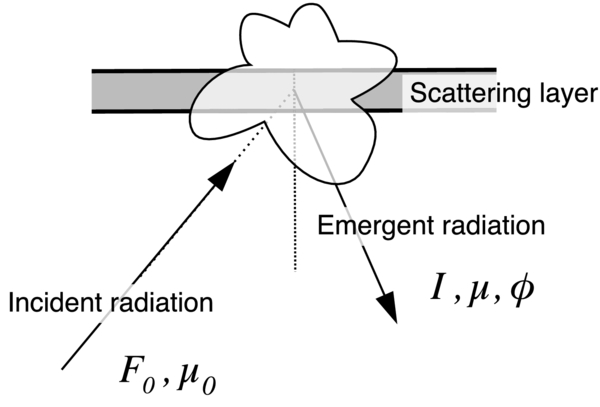
Figure 10. Black-box approach to generalized scattering processes. Mono-directional radiation with a flux parallel to its beam F0 (photons s−1 cm−2) is incident on a plane-parallel scattering layer from a direction μ0 = cos θ0, where θ0 is the angle from the normal to the layer. The azimuth of the incident radiation may be taken as ϕ0 = 0 without loss of generality. The intensity of emergent scattered radiation in a direction μ, ϕ is I (photons s−1 cm−2 sr−1), where the scattered radiation may be in a very different wavelength band from the incident radiation. The effective albedo of the scattering process will depend on the directions of both the incident and emergent radiation and is defined as ϖ(μ0; μ, ϕ) = 4πI/F0.
Download figure:
Standard image High-resolution imageB.1. Formal Calculation of Intensity Ratios and Equivalent Widths
Under this black-box "scattering" or "reprocessing" description, the efficiency of the scattering can be described by an effective albedo ϖeff (see Figure 10), so that the photon intensity I for each line or continuum process is proportional to the local continuum flux F0 in the spectral band that excites the scattering process:
where
In this expression, R is the distance from the star to the scattering layer, and 〈λLλ〉band and (Δλ)band are respectively the mean SED and wavelength width of the continuum band that excite the process. In general, the albedo will be a function of the illumination angle and viewing angle (Figure 10). The particular values of the albedo for the production of the Hβ recombination line, the [N i] fluorescent lines, and dust-scattered continuum in the nebula are calculated in Appendix B.2 below.
The line ratios and equivalent widths measured in Section 2 will then be given by
A particularly simple limiting case is provided by the situation in the extreme outskirts of the Extended Orion Nebula. For these regions studies have shown that, except for the lowest ionization lines, essentially all the radiation, including the emission lines, is scattered by dust rather than being emitted locally (O'Dell & Goss 2009; O'Dell & Harris 2010). For positions far outside the bright core of the nebula, it is reasonable to make the additional assumption that the angular distribution of the incident radiation (as seen by the scatterers) is on average similar for the continuum (which comes from the star cluster) and for the emission lines (which come from the nebular gas). That being the case, all geometrical factors will cancel out and the effective albedo for an emission line will be the same as that for the adjacent continuum, so that the equivalent width of the line will be simply EW(Int) = Lline/Lλ, where Lline is the total intrinsic line luminosity of the nebula and Lλ is the total intrinsic continuum luminosity of the star cluster.7 One would therefore expect that the observed corrected equivalent widths should tend to a constant value of EW(Int) in the extreme outskirts of the nebula. Just such a behavior is seen in the observed Hβ equivalent width (O'Dell & Harris 2010, Figure 8), which around the outer rims of the nebulae tends to a value of ∼150 Å for M42 and ∼100 Å for M43. Comparison with the intrinsic Hβ equivalent widths in Table 2 shows good agreement in the case of the M43, although for M42 the predicted value of 213 Å is rather higher than is observed.
In Table 2 we show SED ratios between different wavebands for OB stellar populations characteristic of the inner Orion Nebula (Trapezium region), the outer Orion Nebula, and M43. These can be compared with different observed emission ratios shown in Figures 1 and 6: FUV/visual corresponds to EW([N i], Corr), EUV/visual corresponds to EW(Hβ, Corr), and FUV/EUV corresponds to I([N i])/I(Hβ).8
B.2. Estimation of Effective Albedos for Particular Processes
B.2.1. Hβ Recombination Line
Assuming a thin, plane-parallel, ionization-bounded layer of dust-free hydrogen that is illuminated by ionizing photons with a flux  (photons s−1 cm−2) incident from a direction μ0, then the condition of global static photoionization equilibrium is given by
in which αB is the "Case B" recombination coefficient and np, ne are the proton and electron densities. At the same time, the emergent intensity I (photons s−1 cm−2 sr−1) of the recombination line Hβ is given by
where αHβ is an effective recombination coefficient that only includes those recombinations that give rise to the emission of an Hβ photon. Combining these, the effective albedo (see Figure 10) is found to be
where 〈αHβ/αB〉 ≃ 0.12 for typical H ii region conditions (Osterbrock & Ferland 2006).
The correction to this result for the presence of helium will be small, but the presence of dust in the ionized gas may have a much larger effect. Both the incident ionizing radiation and the emergent emission line will be affected by dust absorption. The fraction  of ionizing photons that are absorbed by dust is an increasing fraction of the ionization parameter (Aannestad 1989; Arthur et al. 2004), but for the conditions found in Orion reaches a maximum value of about 30% so long as the illumination is close to face-on. The effect is greater for edge-on illumination, but such cases, with μ0 ≪ 1, have already a small albedo and so will contribute little to the observed emission so long as a variety of illumination angles is present (see discussion in Appendix B.3). The absorption of emergent Hβ photons is more important since this is largest for precisely those cases μ ≪ 1 which would give the highest albedo in the dust-free case (Equation (B8)). If the dust absorption optical depth of the scattering layer at the wavelength of Hβ is τ, then in the approximation that the ionized density is constant Equation (B8) becomes
The maximum relative boost in the albedo due to limb brightening as μ → 0, which is infinite in the dust-free case, is now limited to 1/(1 − e−τ), which is a factor of 3–5 for the values of τ ≃ 0.1–0.3 expected in Orion. Note that scattering by dust of the Hβ photons is ignored in this approximation.
B.2.2. Fluorescent [N i]
The FUV fluorescent pumping of the optical [N i] lines is only efficient at wavelengths where the opacity of the pumping line exceeds the background continuum opacity, which at FUV wavelengths is dominated by dust. This gives a limit δλ = λδv/c to the wavelength interval that contributes to the pumping, where δv is of order the Doppler width of the line.9 If there are a number Nline pumping lines, each of effective width δv, then the fraction of the total FUV continuum that contributes to the pumping is  , where
  is the average wavelength of the pumping lines and
  is the wavelength width of the FUV band.10 If a fraction
  of all pumps results in the emission of a line in the optical [N i] λλ5198, 5200 doublet, then the effective albedo for "scattering" of FUV continuum into these lines is
where  and
and  are the continuum absorption optical depths between the star and the pumping layer, measured perpendicular to the layer, and at the wavelengths of the pumping FUV lines and the emerging optical lines, respectively.
The opacity of the FUV pumping lines τpump is proportional to the abundance of N0, and so is very low inside the ionized gas, rising suddenly at the ionization front. Therefore, for strong pumping lines, the fluorescent excitation (which peaks at τpump ≃ μ0), is concentrated in a thin layer just behind the ionization front so that  and
and  are insensitive to variations in the illumination cosine μ0. For the weakest pumping lines, on the other hand, the pumping layer extends deeper into the neutral PDR and so
  and
and  are generally larger and become roughly proportional to μ0.
Figure 11(b) shows results for  for the case of perpendicular illumination μ0 = 1 and assuming Nline = 10, δv = 10 km s−1,
  ,
,  , and
, and  . It can be seen that the same optical depth of dust has a considerably larger effect on the [N i] albedo than on the Hβ albedo, particularly for oblique viewing angles (small μ). This is because the dust absorption layer completely overlies the fluorescent scattering layer in the [N i] case, whereas in the case of Hβ the dust is mixed in with the line-emitting gas. As a result, whereas the Hβ albedo ϖHβ simply saturates at small μ, the [N i] albedo
  has a maximum at
  and then drops to zero as μ → 0.
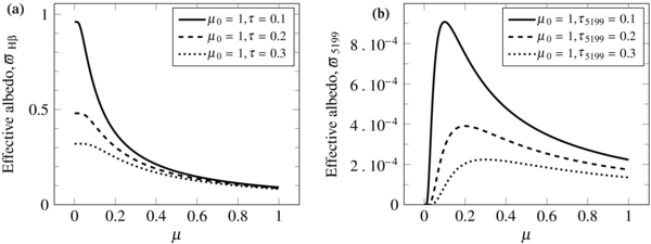
Figure 11. (a) Effective albedo (ϖHβ, Equation (B9)) for "scattering" by a plane ionized layer of normally incident ionizing EUV photons into optical Hβ photons as a function of the viewing direction μ. Results are shown for three different values of τ the perpendicular dust absorption optical depth through the layer at the wavelength of Hβ. The dust acts primarily to limit the limb brightening at small values of μ. Note that ϖHβ is defined in terms of numbers of photons; in terms of energy the values would be a factor  times smaller. (b) Same as (a), but for fluorescent "scattering" of incident FUV photons into optical [N i] photons (
 , Equation (B10)).
Download figure:
Standard image High-resolution imageB.2.3. Scattered Starlight
The dust scattering of starlight in the nebula can be divided into two parts: (1) back-scattering by dust in the PDR and molecular cloud located behind the nebula, which has a high optical depth, and (2) small-angle scattering by dust located in the diffuse clouds in front of the nebula (the neutral veil, Abel et al. 2004, 2006), which has a smaller optical depth (τ = 0.1–1; O'Dell & Yusef-Zadeh 2000). In both cases, the results will be sensitive to the optical properties of the dust grains, which at the simplest level can be characterized by the single-scattering albedo ϖ0, which is the probability that a photon interacting with a grain is scattered rather than absorbed, and the asymmetry parameter g, which is the mean cosine of the scattering angle (g = 0 for isotropic scattering). Dust in Orion is found to have a high value of the total/selective extinction ratio RV ≃ 5, possibly due to grain coagulation (Cardelli & Clayton 1988). Theoretical calculations of the optical properties of a grain population with this value of RV (Figure 4 of Draine 2003) imply that at optical wavelengths (∼5000 Å) the albedo is relatively high (ϖ0 ≃ 0.8) and the scattering is moderately forward-throwing (g ≃ 0.6), whereas at FUV wavelengths (∼1000 Å) the albedo is lower (ϖ0 ≃ 0.4) and the scattering is extremely forward-throwing (g ≃ 0.8). Observations in Orion of scattered FUV continuum (Shalima et al. 2006) and scattered optical emission lines (Section 3.1 of Henney 1998) are consistent with these values, although in both cases it is only a combination of ϖ0 and g that is constrained. Earlier studies (Schiffer & Mathis 1974; Mathis et al. 1981; Patriarchi & Perinotto 1985) have found different values, and even evidence that the dust properties vary with position, but the results are very sensitive to the assumed geometry of the scattering. In the following we present results for both high-albedo and low-albedo grains, which can be taken as representative of the range of possible optical grain properties at visual and FUV wavelengths.
The problem of back-scattering by the molecular cloud has a well-known solution in the case of isotropic scattering (Chandrasekhar 1960), giving an effective albedo of
where H(μ) is the Chandrasekhar H-function. An approximate analytic form for the H-function (Henney 1998), accurate to <5% for ϖ0 ⩽ 0.9, is

For the more relevant case of asymmetric scattering (g ≠ 0), the problem is more difficult to solve, and is no longer axially symmetric unless μ0 = 1. However, for illumination angles that are not far from face-on, a good approximation is found by simply multiplying the isotropic results by a factor of (1 − g)3/2 (Henney 1998). The results of this approximation are shown in Figure 12(a), where it is seen that typical values of  –0.3 are obtained at visual wavelengths, but much smaller values (
 ) are seen at FUV wavelengths. In both cases, the scattering is approximately Lambertian (brightness independent of viewing angle) when the illumination is close to face on. Note however, that this approximation ignores the fact that as μ0 is decreased, then the forward-throwing part of the phase function begins to be sampled at small μ for favorable viewing azimuths ϕ, which would tend to increase the limb brightening for μ0 < 1.
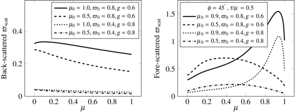
Figure 12. (a) Effective albedos for back-scattering from a very optically thick dusty layer as a function of the viewing angle μ. The upper two lines (solid and dashed) are for optical properties typical of Orion dust at visual wavelengths, while the lower two lines (dotted and dot-dashed) are for those of the same dust at FUV wavelengths, in both cases for two different illumination angles μ0. Note that the approximation used in deriving these curves becomes less accurate as μ0 decreases, as the results start to develop an additional dependency on the viewing azimuth ϕ. (b) Effective albedos for diffuse transmission through a translucent foreground layer with optical depth 0.5 along the line of sight. Line types as in (a).
Download figure:
Standard image High-resolution imageFor the case of forward scattering, one can use the results for diffuse transmission through a homogeneous plane-parallel layer of optical thickness τ (Chandrasekhar 1960), where the effective albedo can be expressed in terms of Chandrasekhar's X and Y functions:
where Φ is the scattering phase function and X and Y depend implicitly on Φ and ϖ0. In the limit of small τ, it is sufficient to include only single scattering, which yields the approximation X(1)(μ, τ) = 1, Y(1)(μ, τ) = e−τ/μ. For multiple scattering in the isotropic case, extensive tables have been published for X and Y (e.g., Mayers 1962) and we find that an acceptable approximation to these results is given by

where
This approximation is accurate to <10% for all the cases covered by Mayers (1962) (τ = 0.1–5, ϖ0 = 0.5–1). To extend this result to forward-throwing phase functions, we assume that the anisotropy can be neglected for all orders of scattering higher than the first, so that Equations (B14) and (B13) may be directly combined.
Example results for scattering from foreground dust in this approximation are shown in Figure 12(b), assuming ϕ = 45° and a Henyey–Greenstein form for the scattering phase function:
The results are shown for a fixed value of the optical depth measured along the line of sight, τ/μ, since it is this quantity that is constrained by observations of the extinction in the neutral veil. Therefore, the actual thickness of the layer τ goes to zero as μ → 0 and no limb brightening is seen. Instead, the albedo tends to have a maximum when μ ≃ μ0 since this maximizes Φ for the small values of ϕ considered here. It can be seen that the effective albedo is generally of order ϖ0τ/μ, although it can be several times larger than this for favorable combinations of μ, μ0, and ϕ that give sufficiently small scattering angles (μs > 0.8 for the optical-band grain properties, or μs > 0.9 for the FUV-band grain properties).
B.3. Variations within the Nebula of the Illumination and Viewing Angles
The effective scattering albedos derived in the previous sections are strong functions of the angle of illumination of the scattering layer μ0 and of the observer's viewing angle μ, with the albedo generally being highest when the illumination is close to face-on (μ0 ≃ 1) and the view is close to edge-on (μ ≃ 0). It is therefore important to consider whether these angles vary systematically between the core and the outskirts of the nebula. This depends critically on the large-scale geometry of the scattering layers within the nebula. For instance, if the nebula were a simple hemispherical shell centered on the Trapezium stars (illustrated in Figure 13(a)), then the illumination angle would be constant at μ0 = 1 while the viewing angle would vary from μ = 1 in the center to μ = 0 at the edge. On the other hand, if the nebula were a plane-parallel layer (as in the models of Henney et al. 2005a and illustrated in Figure 13(b)), then μ would be constant, whereas μ0 would vary from ≃ 1 at the center to ≃ 0 toward the edges. In reality, neither of these simple geometries works well as model for the nebula. In particular, the hemispherical-shell model would predict a constant ionized gas density and a surface brightness that increases with radius, both in violent disagreement with observations. On the other hand, the plane-layer model fails to explain the fine-scale structure seen in many emission lines (e.g., O'Dell & Yusef-Zadeh 2000; García-Díaz & Henney 2007), as well as the sharp edge of the EON. For an observational aperture that is larger than the angular size of the individual emission structures, the observed emission will be biased toward face-on illumination angles and edge-on viewing angles, simply because those are the cases that give the highest effective albedo.
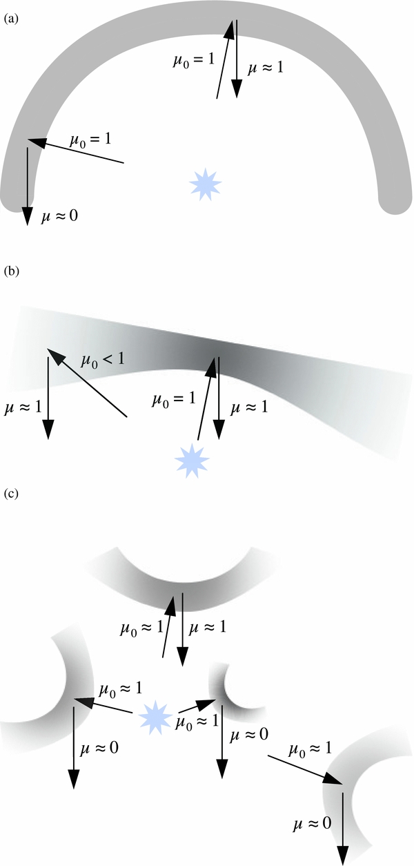
Figure 13. Three simple models for the geometry of the nebula, showing how the illumination angle μ0 and viewing angle μ vary with position in the nebula. In each case, the observer is located off the page to the bottom. (a) A hemispherical shell. (b) A nearly plane layer. (c) An irregular nebula consisting of many globule-like and bar-like features.
Download figure:
Standard image High-resolution imageB.4. Breakdown of the Infinite Plane-parallel Layer Approximation
The results of the previous sections assume that the scattering occurs in a single plane-parallel layer of infinite lateral extent, which is a good approximation so long as the thickness of the each scattering layer and the displacements between them are much smaller than either the distance from the illuminating source, or radius of curvature of the layer, or the size of the observational aperture. Obviously, these conditions will be violated to a greater or lesser extent in a real nebula, which will lead to a variety of additional effects on the line ratios. The most important of these can be characterized as (1) ionization stratification, (2) differential pre-attenuation, or (3) limb-brightening limiting. We now discuss these in turn and show that none of them is likely to have an important effect on the observational results discussed in this paper.
Ionization stratification is the angular separation on the plane of the sky of the different scattering layers, such as the separation of the Hβ emission, which arises in the ionized gas, from the dust-scattered optical continuum, which arises predominantly in the neutral PDR. This stratification is not visible in a true plane-parallel geometry unless the viewing angle is strictly edge-on (μ = 0), but for a finite geometry it will occur for |μ| ≲ z/R where z is the separation between the layers and R is the smaller of the radius of curvature or the lateral extent of the layers. Although ionization stratification will produce fine-scale variations in the line ratios and equivalent widths, it will not affect the values given in Figure 1 unless the angular size corresponding to the inter-layer separation z is larger than the size of the observational sample regions. The sizes of the sample regions are listed in Appendix A of O'Dell & Harris (2010) and range from about 1 to 7 arcmin, which are comfortably larger than the observed inter-layer separations in the regions within 7' of the Trapezium that are included in Figure 1 of this paper.
Pre-attenuation is the reduction of the flux F0 incident on the scattering layer due to absorptions in material at smaller radii that does not contribute to the observed scattered intensity I. In the brightest regions of the nebula it can be shown that the majority of the emission in ionized lines such as Hβ arises in a relatively thin layer near the ionization front (e.g., Wen & O'Dell 1995), but there is also a more extended diffuse component to the emission, which becomes relatively more important at greater distances (Baldwin et al. 1991; Henney et al. 2005a). This pre-attenuation will affect the line ratios and equivalent widths only if it is differential, that is, affecting one scattering process more than another. For incident radiation in the optical and far-ultraviolet bands, the dominant absorption process is always due to dust, whereas for ionizing extreme-ultraviolet radiation it may be dust or hydrogen, depending on the local ionization parameter. In Appendix B.4.1 below it is shown that, in the diffuse ionized gas responsible for the pre-attenuation, dust is the dominant opacity source in the EUV band also. Since the dust absorption cross section is very similar at optical and EUV wavelengths (Figure 19 of Baldwin et al. 1991), pre-attenuation will have almost no effect on EW(Hβ), which is sensitive to the EUV/optical flux ratio. The dust absorption cross section in the FUV band is about 20%–50% higher than in the visual band, so that pre-attenuation may affect EW([N i], Corr), which is sensitive to the FUV/optical flux ratio. However, the total continuum optical depth to the [N i]-scattering layer is only of order unity (see Figure 3) and the optical depth of any diffuse pre-attenuating gas must be substantially less than this, so the effect is likely to be small.
Limb-brightening is the increase in intensity of the emergent intensity as the viewing angle becomes more closely edge-on, due to the increased optical path through the scattering layer. In a strict plane-parallel approximation, the limb brightening does not saturate until the scattering layer is optically thick to the emergent radiation along the viewing direction, but any curvature in the layer will impose an additional limit on the degree of limb-brightening. This arises since the maximum path length through the layer is approximately  , where R is the radius of curvature and h is the layer thickness, meaning that the maximum boost that limb-brightening can give the emergent intensity with respect to the face-on (μ = 0) value is of order
  . Typical values of R/h vary from ≃ 3.5 for the Hβ-scattering layer to ≃ 100 for the [N i]-scattering layer, giving maximum boost factors of ≃ 5 and ≃ 30, respectively. Since optical depth effects also limit the boost factor to a maximum of about 5 (see Appendices B.2.1 to B.2.2 above), the extra limiting of limb-brightening by curvature effects will be unimportant, except arguably for Hβ.
B.4.1. Relative Importance of Dust versus Hydrogen Opacity at EUV Wavelengths
By using the equation of local photoionization equilibrium to rewrite the hydrogen photoabsorption rate in terms of the recombination rate, it is straightforward to show that dust will dominate the EUV opacity in ionized gas for densities less than  , where
  is the EUV dust absorption cross section. Taking
  (Figure 19 of Baldwin et al. 1991) and using the ionizing luminosity of the Trapezium stars listed in Table 1, one finds n' ≃ (7000/D−2) cm−3, where D is the projected distance from the Trapezium in arcminutes (assumed to be on average
  times smaller than the true distance). Coincidentally, this equation for n' is very close to the reference line drawn on Figure 6 of O'Dell & Harris (2010), which shows observationally derived electron densities as a function of distance, and from which it can be seen that n < n' for D < 2' but that n ∼ n' for D = 2'–7'. The diffuse ionized gas in the interior of the H ii region is likely to have somewhat lower density than the mean densities derived from line ratios. Therefore, we conclude that dust is the dominant opacity source for EUV radiation in the diffuse ionized gas at all radii covered by our observations.
Note, however, that this does not mean that dust is the dominant EUV opacity source in the H ii region as a whole. In fact, only 10%–20% of the ionizing photons are absorbed by dust, but the hydrogen absorption is weighted toward the edge of the H ii region, rather than the diffuse interior gas.
APPENDIX C: NON-THERMAL LINE BROADENING OF [N i] AND OTHER LINES
In the Orion Nebula, as elsewhere in the interstellar medium, significant non-thermal line widths are observed to be ubiquitous in all gaseous phases (O'Dell 2001; O'Dell et al. 2003). This is shown in Table 12, which collates measurements from the literature of line widths δV and gas temperature T for various emission lines in the central Orion Nebula, ranging from fully molecular to fully ionized species. The expected thermal FWHM is  where T is the temperature in K and A is the atomic weight of the emitting species in units of the proton mass mp. This is subtracted in quadrature from the total width to give the non-thermal broadening component:
  . It can be seen that the non-thermal component dominates over the thermal in all cases and increases in magnitude from about 3 km s−1 in fully molecular gas up to about 15 km s−1 in the fully ionized gas. If the non-thermal broadening is truly due to gas motions, then an approximate characteristic Mach number of these motions can be calculated as M = 0.5 δVnth/cs, where
  is the sound speed and μ is the mean mass per particle. This Mach number is shown in the last column of the table, and in contrast to the line width it decreases with increasing ionization of the gas: the non-thermal motions are highly supersonic in fully molecular gas, slightly supersonic in the PDR, and slightly subsonic in the ionized gas.
Table 12. Non-thermal Line Widths of Different Gas Phases in Orion
| Atomic | Mean | Gas | Sound | Line Width FWHM | Mach | |||
|---|---|---|---|---|---|---|---|---|
| Weight | Mass | Temperature | Speed | Total | Thermal | Non-thermal | Number | |
| Species | A | μ | T (K) | cs (km s−1) | δV (km s−1) | δVth (km s−1) | δVnth (km s−1) | M |
| CO | 28 | 2.36 | 40 ± 10 | 0.37 ± 0.05 | 3.0 ± 0.5 | 0.26 ± 0.03 | 2.99 ± 0.50 | 4.0 ± 0.9 |
| [C ii] | 12 | 1.30 | 400 ± 100 | 1.59 ± 0.20 | 4.0 ± 1.0 | 1.23 ± 0.15 | 3.81 ± 1.05 | 1.2 ± 0.4 |
| [N i] | 14 | 1.30 | 2000 ± 500 | 3.56 ± 0.45 | 6.0 ± 3.0 | 2.56 ± 0.32 | 5.43 ± 3.32 | 0.8 ± 0.5 |
| [O i] | 16 | 0.90 | 9500 ± 500 | 9.33 ± 0.25 | 12.6 ± 2.4 | 5.21 ± 0.14 | 11.47 ± 2.64 | 0.6 ± 0.1 |
| [N ii] | 14 | 0.68 | 9000 ± 500 | 10.45 ± 0.29 | 16.3 ± 3.5 | 5.42 ± 0.15 | 15.37 ± 3.71 | 0.7 ± 0.2 |
| [O iii] | 16 | 0.65 | 8400 ± 500 | 10.33 ± 0.31 | 15.5 ± 4.8 | 4.90 ± 0.15 | 14.71 ± 5.06 | 0.7 ± 0.2 |
Notes. All line widths have been corrected for instrumental broadening. References. CO: Wilson et al. 2001; [C ii]: Boreiko et al. 1988; other lines: Baldwin et al. 2000; García-Díaz et al. 2008.
Download table as: ASCIITypeset image
Optical and infrared emission lines from H ii regions and PDRs, such as the majority of those listed in Table 12 are usually optically thin. Therefore, the observed line widths give no information about the spatial scales at which the broadening mechanism operates. On the other hand, for optically thick lines, such as the FUV lines that are responsible for pumping the [N i] emission, one can divide potential broadening mechanisms into two categories: microscopic and macroscopic, according to whether they occur at scales that are smaller than or larger than the relevant photon mean free path. Of the two, only microscopic mechanisms act to broaden the absorption profile and so affect the radiative transfer of the line, whereas macroscopic mechanisms simply act to broaden the emergent intensity profile.
The line broadening that we derive for the pumping lines in order to explain the observed optical [N i] line brightness (see Figure 5) is similar to, but smaller than, the broadening observed in the lines themselves (Table 12), implying that the non-thermal broadening mechanism must be microscopic in nature. In other words, it should occur on scales of less than 1014 cm, which is the approximate mean free path of the 954 Å pumping line.
In the H ii region, transonic turbulence is expected to be driven at the scales of photoevaporation flows from dense globules and filaments (Mellema et al. 2006; Arthur et al. 2011; Ercolano et al. 2012). The most vigorous photoevaporation flows only occur at scales larger than about 10% of the H ii region radius (Henney 2003). In the Orion Nebula, the closest approach of the ionization front to the ionizing stars is about 0.2 pc (Wen & O'Dell 1995), so we assume that turbulent velocities of amplitude 11 km s−1 are present at scales of 0.02 pc, or 6 × 1016 cm. In a Kolmogorov-type turbulent energy cascade, velocity differences scale with separation ℓ as δv ∼ ℓ1/3. Therefore, on the scale of the N i mean free path the turbulent broadening should be only approximately 1 km s−1, which is much smaller than our derived microscopic broadening, which means that this is not the mechanism we seek.
A further potential source of broadening is the systematic acceleration of the gas as it is dissociated, heated, and ionized by the advancing front. However, the [N i] emission arises in regions where the gas is still predominantly neutral, with temperature ranging from 1000 to 5000 K (see Figure 3), for which the velocity increase is expected to be small since the greater part of the gas acceleration occurs in the warmer, partially ionized zone where the [O i] lines arise. For example, a plane-parallel model of a D-critical ionization front (Equations (A5)–(A8) of Henney et al. 2005b) implies a total broadening FWHM for the [N i] lines of less than 2 km s−1 by this process.
We therefore see that none of the broadening mechanisms that have been successfully invoked to explain the observed widths of neutral and ionized collisional lines are successful in explaining the observed characteristics of the fluorescent [N i] lines. Other potential mechanisms such as instabilities of the ionization front itself (Williams 2002; Whalen & Norman 2008) are not promising either, since they are unlikely to produce microturbulence at a sufficiently small scale. Neither can broadening due to dust scattering in the neutral veil (Henney 1998) be the explanation, since this would have no affect on the radiative transfer of the N i pumping lines.
A more promising mechanism for generating turbulent velocities on a very small scale is the action of thermal instabilities (Koyama & Inutsuka 2002) in the shocked neutral layer that precedes the ionization front. It is suggestive that the temperature range over which the [N i] lines form in the PDR (1000–3000 K) is similar to the range over which the ISM is known to be thermally unstable (Field et al. 1969). If such an instability were to occur in the PDR, then the smallest scale at which fragments could arise (and hence turbulence be driven) is given by the Field length λF (Field 1965), which represents the scale below which temperature fluctuations will be smoothed out by thermal conduction. Assuming saturated conduction by free electrons (Zel'Dovich & Raizer 1967), one finds a value of λF ≃ (1015/n) cm, which is roughly 100 times smaller than the thickness of the [N i] pumping layer. The role of thermal instability in generating the required microscopic non-thermal broadening therefore merits further investigation.
Footnotes
- 6
The [O i] 6300 Å emission is more complicated because of a strong dependence on the ionization parameter, and so will not be considered further here.
- 7
As described in Section 2, the contribution to the observed equivalent widths of the atomic continuum emission from the nebular gas should first be corrected for.
- 8
Note that only two of these three quantities are independent.
- 9
For a Gaussian line profile,
 , where b = 0.601 × FWHM is the Doppler broadening parameter, k0 is opacity at line center, and is the continuum dust opacity.
 - 10
For the wavelength range of 950–1200 Å used in Table 2,
.
