


ABSTRACT
Magnetic loops are building blocks of the closed-field corona. While active region loops are readily seen in images taken at EUV and X-ray wavelengths, quiet-Sun (QS) loops are seldom identifiable and are therefore difficult to study on an individual basis. The first analysis of solar minimum (Carrington Rotation 2077) QS coronal loops utilizing a novel technique called the Michigan Loop Diagnostic Technique (MLDT) is presented. This technique combines Differential Emission Measure Tomography and a potential field source surface (PFSS) model, and consists of tracing PFSS field lines through the tomographic grid on which the local differential emission measure is determined. As a result, the electron temperature Te and density Ne at each point along each individual field line can be obtained. Using data from STEREO/EUVI and SOHO/MDI, the MLDT identifies two types of QS loops in the corona: so-called up loops in which the temperature increases with height and so-called down loops in which the temperature decreases with height. Up loops are expected, however, down loops are a surprise, and furthermore, they are ubiquitous in the low-latitude corona. Up loops dominate the QS at higher latitudes. The MLDT allows independent determination of the empirical pressure and density scale heights, and the differences between the two remain to be explained. The down loops appear to be a newly discovered property of the solar minimum corona that may shed light on the physics of coronal heating. The results are shown to be robust to the calibration uncertainties of the EUVI instrument.
Export citation and abstract BibTeX RIS
1. INTRODUCTION
Magnetic loops are building blocks of the magnetically closed solar corona. They host the plasma as well as the processes that heat it, and their interactions with open field lines may even generate the fast and slow solar wind (Fisk et al. 1999; Wang et al. 1998; Feldman et al. 2005; Antiochos et al. 2011). Despite their importance, they are not yet well understood; in particular, we do not know exactly which mechanisms heat the plasma, not even whether it is a steady heating (Warren et al. 2010; Winebarger et al. 2011; Schrijver et al. 2004) or an impulsive, nanoflare heating (Viall & Klimchuk 2011; Patsourakos & Klimchuk 2005). Despite the fact the quiet Sun (QS) can cover the vast majority of the solar surface, especially near the cycle minimum, almost all of the work on coronal loops has only considered active region (AR) loops, and QS loops are a largely unexplored territory. We are not aware of any published studies of individual QS loops. This state of affairs is partially due to the fact that ARs are more likely to be hosts of dramatic events such as powerful flares and coronal mass ejections, and to the fact that it is very difficult, if not impossible, to observationally define a QS loop in an EUV (although one could argue that QS loops are seen in the processed white-light eclipse images of Pasachoff et al. 2011), while they are readily identified in ARs (e.g., Vaiana et al. 1973; Aschwanden & Boerner 2011). The difficulty in observing QS loops is perhaps related to the fact that loops become "fuzzy" when seen in high temperature lines (Tripathi et al. 2009), which is explained by Reale et al. (2011) in terms of impulsively heated independent strands (which spend most of their time at coronal temperatures). The QS corona has mostly been studied by applying plasma diagnostic techniques to spatially averaged regions of the corona with no attempt to resolve individual loop structures. The QS analyses reviewed by Feldman & Landi (2008; see also Feldman et al. 1999; Warren 1999; Landi et al. 2002) have shown a nearly isothermal solar corona with little time evolution, but this can be an artifact of time averages of the observations. At larger heights (1.7 R☉), Raymond et al. (1997) used UVCS/SOHO (Kohl et al. 1995) data for an abundance analysis of a solar minimum equatorial streamer and found that an isothermal plasma at 1.6 MK explains the observations, although the possibility of hotter and cooler plasma cannot be excluded.
In the present effort, we demonstrate a new method that allows identification of QS loops for the first time and provide first results of some of their properties, including the first observational identification of loops in which the temperature decreases with height.
2. DATA AND MLDT ANALYSIS
Here, we assume that QS loops are well described by potential fields between 1.03 and 1.20 R☉ and determine the three-dimensional (3D) electron temperature Te and density Ne in this height range using the Differential Emission Measure Tomography (DEMT) technique (Frazin et al. 2005, 2009; Barbey et al. 2011). In DEMT, solar rotation tomography (SRT) is applied to a time series of multi-band EUV images, such as those provided by EUVI (Howard et al. 2008) or Atmospheric Imaging Assembly. If multiple spacecrafts are used, this can be accomplished in less than a full synoptic rotation period. After the SRT has been performed, a standard differential emission measure (DEM) analysis technique is applied to produce the local differential emission measure (LDEM).3 The LDEM's (normalized) 0th and 1st moments are 〈N2e〉 and Tm ≡ 〈Te〉, where the brackets 〈 〉 denote the volume average over a voxel in the tomographic grid (although, technically, 〈Te〉 is a volume average weighted by N2e, as can be see seen in the Appendix C of Frazin et al. 2009). The Michigan Loop Diagnostic Technique (MLDT) takes a field line specified by a potential field source surface model (PFSSM) and follows it through the tomographic grid, assigning the DEMT values of (〈N2e〉)1/2 and Tm to all of the points along the loop. We use the synoptic magnetogram provided by MDI/SOHO on the 3600 × 1080 longitude/latitude grid, binned to 360 × 180. As we only consider the field above 1.03 R☉, more resolution is not necessary. Our PFSSM model was developed by Tóth et al. (2011), and it uses a finite-difference solver to calculate the magnetic field and provides a more accurate field in high latitude regions than are typically obtained with expansion methods. The MLDT was first applied to test the hypothesis of hydrostatic equilibrium in open and closed field structures for several regions in CR2068 (also near solar minimum) in Vásquez et al. (2011). There it was found that in open field regions, the ion temperature was higher than the electron temperature (Tm) or significant wave pressure gradients must exist, while the closed region data seemed to be much more consistent with isothermal (i.e., equal electron and ion temperatures) hydrostatic equilibrium.
Development of the MLDT makes us the first to identify individual QS loop bundles and measure their thermodynamic states, and it also allows statistical studies of their properties. The most important limitation of the MLDT is temporal resolution specified by the full solar rotation (∼27.3 days) required to make the synoptic magnetogram for the PFSSM. DEMT has a similar limitation, but in this case the dual-spacecraft STEREO geometry allowed us to acquire the equivalent of a synoptic rotation in about 21 days. The QS is particularly well suited to using DEMT and the PSSFM because, while there are fluctuations on rapid timescales, QS regions show little secular evolution and they seem to be statistically stationary, so the time averages are meaningful approximation of their states. Furthermore, the results presented below are based on statistical analyses of hundreds of loops, and our conclusions are based on statistical trends, so that the particular dynamics of any single loop are not important. Also, it is likely that any sporadic currents in QS regions are on small spatial scales in the chromosphere or below and have a negligible influence on the large-scale field studied here, thus supporting the use of the PFSSM.
In the present paper, we apply the MLDT to CR2077, which corresponds to the period between UT 06:56 November 20 and UT 14:34 2008 December 17, a time of extremely low solar activity as the sunspot minimum was achieved in the next Carrington rotation. CR2077 had only one short-lived AR (NOAA 11009, December 11–13), so the Sun was very quiet and nearly ideal for our analysis. The region corresponding to the AR was excluded from this analysis.
During this period, the two STEREO spacecrafts were separated by 84 5 ± 12, which allowed for the reconstruction to be performed with data gathered in about 21 days (around 3/4 of a solar rotational time). The data consist of hour cadence EUVI images in the 171, 195, and 284 Å bands taken from UT 00:00 2008 November 20 to UT 06:00 2008 December 11, co-added to make one image every 6 hr that was processed by the SRT code. SRT is independently performed for the series of images corresponding to each wavelength band resulting in the 3D distribution of the filter band emissivity (FBE) for each band. The FBE is an emissivity defined in Frazin et al. (2009), and it can be obtained by integrating the LDEM with the appropriate temperature weighting function. It plays a role that is analogous to the observed spectral line intensity in standard DEM analysis (Craig & Brown 1976). While the DEM and intensity are line-of-sight integrated quantities, the LDEM and the FBE pertain only the plasma located within a given voxel of the tomographic grid. The SRT technique does not account for the Sun's temporal variations (although, see Butala et al. 2010), and rapid dynamics in the region of one voxel can cause artifacts in neighboring ones. Such artifacts include smearing and negative values of the reconstructed FBEs, or zero when the solution is constrained to positive values. These are called zero-density artifacts (ZDAs) and are similar to those described by Frazin & Janzen (2002) in white-light SRT. As is common, some of the ZDAs that appear in this reconstruction correspond to the location of the AR. For all voxels with no ZDAs, we use the inferred LDEM to forward compute the three synthetic values of the FBE. We only use the voxels where the synthetic and measured values agree within 1%, which happens to be the vast majority of them.
The STEREO calibration has not been addressed in any publication since Howard et al. (2008), but (J. P. Wuelser 2011, private communication):
- 1.The drift in instrumental sensitivity with time is negligible.
- 2.The relative calibration of the EUVI channels has an uncertainty of 15%. In Section 4, we show that this uncertainty has little effect on our results.
- 3.The absolution calibration has an uncertainty of about 30%. This uncertainty has the potential to change the electron density estimates uniformly by ∼15%, and it does not affect the temperature determinations, so it is of little importance for this analysis.
Another limitation comes from the optical-depth issues in the EUV images, especially in the 171 Å band, close to the limb band (Schrijver et al. 1994). To avoid optical depth issues, we do not utilize the EUVI image data between 0.98 and 1.025 R☉, as explained in Appendix D of Frazin et al. (2009). Due to the data rejection in this annulus and the consequent loss of information, we treat the tomographic reconstructions to be physically meaningful above heliocentric heights of 1.03 R☉.
The spherical computational grid covers the height range 1.00–1.26 R☉ with 26 radial, 90 latitudinal, and 180 longitudinal bins, each with a uniform radial size of 0.01 R☉ and a uniform angular size of 2° (in both latitude and longitude). It is not useful to constrain the tomographic problem with information taken from view angles separated by less than the grid angular resolution. Therefore, as the Sun rotates about 132 per 24 hr period, we time average the images in 6 hr bins, so that each time-averaged image is representative of views separated by about 33. Also, due to their high spatial resolution (1 6 pixel−1), to reduce both memory load and computational time, we spatially rebin the images by a factor of eight, bringing the original 2048 × 2048 pixel EUVI images down to 256 × 256. Thus, the final images pixel size is about the same as the radial voxel dimension. The statistical noise in the EUVI images is greatly reduced because of this spatial and temporal binning. Even so, the maximum height we consider is 1.20 R☉, as the reconstructions tend to be problematic above that height due to the weaker coronal signal.
The electron temperature of a given point on a magnetic field line from the PFSSM can be determined from the DEMT temperature (Tm) data. We trace individual field lines through the tomographic grid to obtain the temperature profile along the field line. This temperature profile is representative of the bundle of field lines that pass through the tomographic cells. The field line integration begins at the height of 1.075 R☉, in the center of the radial bin that begins at 1.07 and ends at 1.08 R☉, so that only field lines with apexes at 1.075 R☉ or higher are considered. (The field line is traced in both the parallel and anti-parallel directions, so that the entire loop is determined.) This choice was made because we discard the tomographic data in the three cells between 1.0 and 1.03 R☉ due to optical depth effects,4 and we require each leg of the loop to pass through at least five tomographic cells above 1.03 R☉ in order to be included in this analysis5. One effect of starting the field line integration at 1.075 R☉ is to avoid the low-lying small loops since any field lines closing below that height will not be seen. Open field lines are not considered in this analysis, although some previous results can be found in Vásquez et al. (2011).
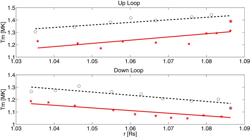
For each field line i, we determine T(i)m(r), where r is the heliocentric height, in each tomographic voxel along the loop. We then fit the T(i)m(r) profile with a linear function

where the temperature gradient a and intercept b are the two free fitting parameters. "Up" loops are those field lines for which a > 0, implying that the electron temperature increases with height and, and "down" loops are those for which a < 0, implying that the electron temperature decreases with height. Figure 1 shows a least-squares fits to a typical up loop and a typical down loop. The quality-of-fit metric we used is called R2 and is commonly known as the coefficient of determination.6 The maximum attainable value of R2 is unity which can only be achieved when the fitted curve exactly agrees with all data points. We generated magnetic field lines every 2° in latitude and longitude from the PFSS model, for a total of 16,200 loop foot-points. Of these, most were rejected for one or more of the following reasons.
- 1.The field line is open according to the PFSSM.
- 2.The field line is in, or too close to, the AR.
- 3.The fitted temperature gradients a of the two loop legs do not have the same sign.
- 4.The quality of the linear fit, R2 < 0.5 for either leg of a loop.
- 5.One of the two loop legs does not go through at least five tomographic grid cells with usable data.
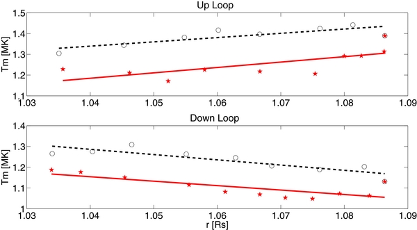
Figure 1. Linear least-squares fits of the form Tm = a r + b to determine loop classification as "up" (a > 0), or "down" (a < 0). Top: two legs of a up loop, with black circles representing the DEMT Tm values of one leg and red stars representing the other. The red solid line is the fit to the red stars and the black dashed line is the fit to the black circles. Bottom: similar to the top panel, but for a down loop. The black dashed and red solid curves in the upper and lower panels have quality-of-fit values R2 of 0.67, 0.51, 0.76, and 0.59, respectively. Since we only accept loops with R2 > 0.5 (for this stage in the analysis), these fits are fairly typical.
Download figure:
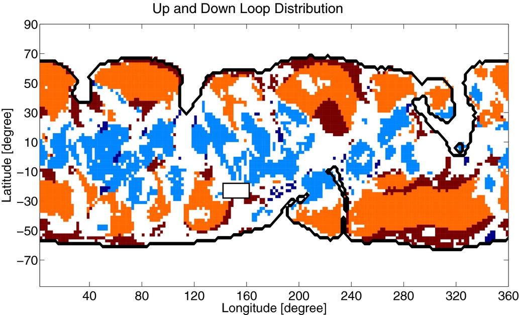
Standard image High-resolution imageConsequently, there are about 4600 loop legs left to examine the spatial distribution of up and down loops. We find that up loops are mostly located in high latitude regions and down loops in low latitude regions, as shown in Figure 2, which displays this spatial distribution at 1.075 R☉. Because the LDEM data are considered to be good up to about 1.2 R☉ for this data set, we separate both the up and down into large and small loops. A large loop is a field line with its apex beyond 1.2 R☉ and a small loop has its apex below 1.2 R☉, which means that the large loops do not have data for their portions above 1.2 R☉. The light blue areas in this figure are threaded by small down loops and the dark blue areas by large down loops. The orange areas are threaded by small up loops and red areas by large up loops. To better understand the foot-point distribution at the solar surface, we traced the loops to the solar surface to determine the latitude of the foot-point of each loop. We find that 96% of the down loops are located within ±30° latitude and 78% of up the loops are outside ±30° latitude, as shown in Table 1. (In this table, only legs with R2 > .9 in the hydrostatic fitting (see Section 3) are included.) A 3D view of up and down loops is displayed in Figure 3. The white lines are open field lines, which are excluded in this study. The red lines are up loops and blue lines are down loops. The field line integration code provides information about the loops, including their lengths. In this article, the length of a loop L is defined as the foot-point-to-foot-point distance along the potential field line connecting them. Figure 4 shows histograms of the lengths of the up and down loops in Figure 2. While up loops are more likely to have lengths greater than about 0.5 R☉, both histograms have large populations below that length.

Figure 2. Spatial distribution of up and down loops at 1.075 R☉ with R2 > 0.5 for the linear temperature fit (Equation (1); Figure 1). The blue regions are threaded by down loops while the orange and dark red regions are threaded by up loops. Dark blue and dark red represent regions threaded by loops with apexes above 1.2 R☉, while light blue and orange represent loops with apexes below 1.2 R☉. The solid black line represents the boundary between open and closed field according to the PFSSM, and the white regions are excluded from our analysis for reasons listed in the text. The box near (−20, 150) contains NOAA active region 11009.
Download figure:
Standard image High-resolution image
Figure 3. Three-dimensional representation of the up and down loop geometry, with red and blue depicting up and down loops, respectively. The spherical surface has a radius at 1.035 R☉ and shows the LDEM electron temperature Tm according to the color scale.
Download figure:
Standard image High-resolution image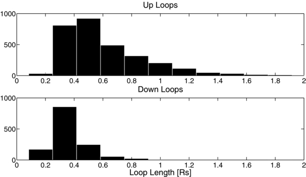
Figure 4. Histogram showing the distributions of loop lengths for the up (top panel) and down (bottom panel) loops, whose spatial distribution is displayed in Figure 2. While an up loop is more likely to be longer than about 0.5 R☉, these distributions indicate that length cannot be the primary discriminating factor between up and down loops.
Download figure:
Standard image High-resolution imageTable 1. Statistical Quantities of Small/Large Up/Down Loops
| Number of Loop Legs | % of Foot-points | % of Foot-points | Average Loop | Average N0 | Average P0 | Average λN | Average λP | Average ∂Tm/∂r | |
|---|---|---|---|---|---|---|---|---|---|
| Within ±30° latitude | Outside ±30° Latitude | Length (R☉) | (108 cm−3) | (10−3 Pa) | (R☉) | (R☉) | (MK R☉−1) | ||
| Small Up Legs | 4155 | 20 | 80 | 0.5 | 2.2 | 7.1 | 0.082 | 0.101 | 2.89 |
| Large Up Legs | 1255 | 42 | 58 | 1.46 | 1.9 | 6.2 | 0.095 | 0.114 | 1.73 |
| Small Down Legs | 2585 | 97 | 3 | 0.36 | 2.3 | 8.6 | 0.082 | 0.064 | −3.7 |
| Large Down Legs | 57 | 86 | 14 | 1.27 | 2.2 | 8.2 | 0.082 | 0.071 | −1.87 |
Note. N0 and λN are the base density and density scale height, respectively, and P0 and λP are the base pressure and pressure scale height, respectively (see Equations (2) and (4)).
Download table as: ASCIITypeset image
3. SCALE-HEIGHT ANALYSIS
It is well known that an isothermal hydrostatic plasma has an exponentially decreasing pressure distribution. A plasma is considered to be effectively hydrostatic when it is in steady state and the inertial term is not important in the momentum equation. In the absence of temperature gradients, the hydrostatic solution to the 1D spherical momentum equation is given by
where r is the spherical radial coordinate, P is the pressure, P0 is the pressure at 1.0 R☉, and λP is the pressure scale height. The relationship between the pressure scale height and the total kinetic temperature is λP = kBT/(μmHg☉), where μ = (1 + 4a)/(1 + 2a) is the mean atomic weight per electron, a = N(He)/N(H) is the helium abundance, g☉ = GM☉/R2☉, and G, mH, M☉, and kB are the gravitational, proton mass, solar mass and Boltzmann constants, respectively. The total kinetic temperature is given by

where TH is the proton temperature and THe is the α particle temperature. If we take a = 0.08 and further assume Te = TH = THe, we find that Te ≈ 0.52 T. Similarly, the electron density profile is given by the equation
where Ne0 is the electron density at 1 R☉ and λN is the density scale height. Of course, under these assumptions λN = λP.
As DEMT provides us with empirical measures of both Ne and Te, comparing fitted values of λN to λP for a number of loops gives us the opportunity to test the assumptions under which Equations (2) and (4) are derived. In Vásquez et al. (2011), for many loops, we compared the loop-averaged value of Te from DEMT ("Tm" in that paper) to the value of 0.52 T ("Tfit"), which was derived from a fitted value of λN to the Ne values, also from DEMT. In that paper, we found that in the closed field regions the histogram Tfit–Tm was clustered around 0, seemingly consistent with isothermal hydrostatic equilibrium. However, in the open field regions, the histogram Tfit–Tm was clustered around a positive value, providing evidence for wave pressure gradients and/or having ions with higher temperatures than the electrons.
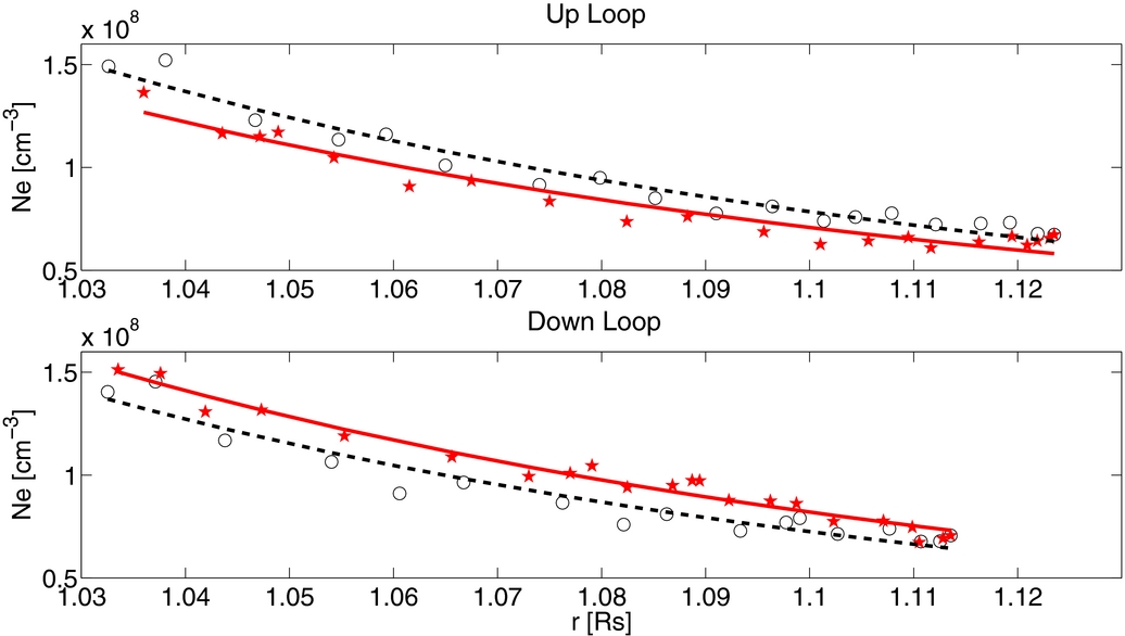
The loop study presented here is similar but attempts to provide an improved analysis, by taking advantage of our knowledge of the temperature variation along each loop. In Vásquez et al. (2011), Tm represented the average (measured) Te along the loop and did not take into account the measured temperature variations along the loop. As before, λN is fit to the Ne values for a given loop in this analysis. Figure 5 shows examples of these fits. New to this analysis, λP is fit to the measured pressures along each loop, with the pressure in the jth tomographic cell given by

where C ≡ kB[(2 + 3a)/(1 + 2a)], and Ne(rj)and Te(rj) are the DEMT values in cell j. Figure 6 shows two examples of fits to determine λP. We removed the legs that have bad hydrostatic fits (R2 < .9 for either density or pressure fitting.) Figure 7 shows a histogram of the differences between the two scale heights, λN and λP, where it can be seen that almost all of the up loops have λP > λN, while almost all of the down loops have λP < λN. It is not surprising that up loops have λP > λN, and vice versa, as it follows from qualitative consideration of Equations (1) and (4): given that the exponential model in Equation (4) fits the data well, a positive temperature gradient will produce greater pressure at large heights than would be seen in an isothermal loop, thus making λP > λN. The opposite argument can be made for loops with negative temperature gradients.

Figure 5. Upper and lower panels give examples of fits to determine the base density Ne0 and density scale height λN, for an up and a down loop, respectively (Equation (4)). The data points are the DEMT values of the electron density Ne. The symbols and line styles are as in Figure 1. The black dashed and red solid curves in the upper and lower panels have quality-of-fit values R2 of 0.95, 0.94, 0.92, and 0.97, respectively. Since we only accept loops with R2 > 0.9 for the scale-height analysis, these fits are fairly typical.
Download figure:
Standard image High-resolution image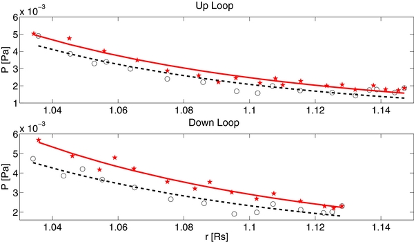
Figure 6. Upper and lower panels give examples of fits to determine the base pressure P0 and pressure scale height λP, for an up and a down loop, respectively (Equation (2)). The two loops shown here are the same two loops that are displayed in Figure 5. The data points are values of pressure determined from DEMT temperature and density using Equation (5). The black dashed and red solid curves in the upper and lower panels have quality-of-fit values R2 of 0.89, 0.94, 0.91, and 0.96, respectively. Since we only accept loops with R2 > 0.9 for the scale-height analysis, these fits are fairly typical.
Download figure:
Standard image High-resolution image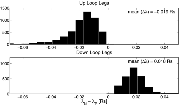
Figure 7. Top and bottom panels show histograms of the scale-height differences λN − λP (see Equations (2) and (4)) for the legs of the up loops and down loops, respectively. The two histograms are plotted on the same horizontal scale. As expected, almost all of the up loops have λP > λN, while almost all of the down loops have λP < λN.
Download figure:
Standard image High-resolution image4. DISCUSSION AND CONCLUSIONS
We study QS loops at solar minimum with apexes at 1.075 R☉ or greater using the new MLDT, which combines DEMT and a PFSS model. This investigation has yielded three principal results.
- 1.Much of the QS is populated with "down" loops, in which the temperature decreases with height. "Up" loops, in which the temperature increases with height, are expected but down loops are a surprise.
- 2.The down loops are ubiquitous at low latitudes, while the up loops are dominant at higher latitudes, closer to the boundary between the open and closed magnetic field (see Figure 2.)
- 3.The MLDT allows independent determination of the empirical pressure and density scale heights, λP and λN, respectively (see Figure 7).
One may question whether or not the down loops are simply an artifact of the MLDT and therefore do not exist on the Sun. We believe the Sun does exhibit down loops and that they are not an artifact of the MLDT, which is primarily limited by the similar temporal resolutions of the synoptic magnetogram and SRT, and the results presented are robust to the EUVI calibration uncertainties (see the Appendix). The various assumptions made in this analysis, while questionable for individual field lines, should be adequate to extract broad statistical trends, especially in QS plasma at solar minimum, and it is difficult to explain the trends shown here as non-physical.
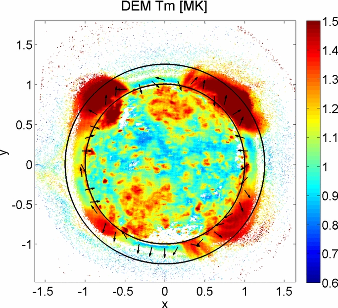
To give our arguments more strength, we performed a non-tomographic DEM analysis, avoiding the temporal resolution issue (at the expense of loosing the 3D information from the tomography). This is shown in Figure 8, which is an image of the temperature derived from a traditional DEM analysis in two spatial dimensions. We averaged 6 hr images in the 171, 195, and 284 Å bands taken by EUVI-A between 6:00 and 12:00 on 2008 December 9. (At 9:00, the central longitude of the solar disk was about 151°.) Similar to the method used to calculate the LDEM, we assumed that the DEM has a Gaussian form with the free parameters being the height, centroid location, and width (see also Aschwanden et al. 2011). Figure 8 is an image of the DEM mean temperature Tm, and the arrows indicate the 2D temperature gradient. Downward gradients can be seen near the equator on both the E and W limbs, supporting the existence of down loops. Upward temperature gradients, likely indicating up loops, can be seen at larger latitudes.

Figure 8. Determination of the DEM without tomography from 6 hr images taken by EUVI-A between 6:00 and 12:00 UT on 2008 December 9. The longitude of the central meridian was about 151°. Displayed is the mean of the DEM, Tm, which corresponds to the average electron temperature along the line of sight. The black arrows indicate the direction of the 2D gradient of Tm in the image plane. The arrows that point radially inward near the and E and W limb are consistent with our finding of down loops. The inner and outer circles are at 1.0 and 1.2 R☉, respectively.
Download figure:
Standard image High-resolution imageWith angular and radial spans of 2° × 2° × 0.01 R☉, the tomographic grid cells are much larger than the smallest observed widths of AR loops (<1000 km), and one may wonder whether or not the down loops are an artifact of the spatial resolution and averaging over many elemental loops of different heights and temperatures. This seems unlikely since the loops we consider here have apexes above 1.075 R☉, where the potential magnetic field does not have large gradients. Thus, all of the elemental field lines passing through a tomographic grid cell at this height must be roughly parallel and averaging over the volume of a tomographic grid cell includes mostly loops of similar geometry.
Serio et al. (1981) arrived at a down loop solution, with a temperature minimum at the apex, but they concluded this solution would cause instabilities to destroy the loop when the loop half-length (the length of one leg), L/2, is greater than ∼2–3 times the pressure scale height. If the loop length is small enough to keep the loop stable, then this solution is related to prominence formation. With average down loop lengths about six times the average scale heights (for the small loops) in Table 1, the data do not seem to support the loop destruction hypothesis, but this needs to be examined more closely. Aschwanden & Schrijver (2002) also found a down loop solution, but they did not discuss this solution in detail, as most loops were thought to be up loops. However, our results show that down loops are ubiquitous at low latitudes (see Table 1). Balancing electron heat conduction, radiative losses, and ad hoc heating, the hydrostatic loop model developed by Aschwanden & Schrijver (2002) shows that the height of the loop temperature maximum moves downward as sH/L decreases, where sH is the (exponential) heating scale length. Within this paradigm, down loops exist because sH is much smaller than the loop length, meaning the heating is localized at the foot-point and the only process available to heat the apex is electron heat conduction. Up loops then are indicative of the heating scale length sH being close to or larger than the loop length, implying roughly uniform heating along the loop. If the hydrostatic model developed by Aschwanden & Schrijver (2002) is descriptive of the real Sun, and if we assume that sH is independent of latitude, then one would expect loop length to be an excellent discriminator of up and down loops. However, this does not seem to be the case, as Figure 4 shows that both up and down loops have large populations between 0.15 (the shortest length allowed in this analysis) and 0.5 R☉, and that any loop length less than about 1 R☉ is not a key variable in distinguishing the two populations. That said, the figure also shows that loops longer than about 1 R☉ are very likely to be up loops. Table 1 also indicates that the up loops tend to be longer than down loops, which is a direct contradiction of the hypothesis of hydrostatic loops with a scale height that is independent of foot-point location. The most reliable predictor of the up and down loop distribution is the foot-point latitude. Thus, if the QS plasma is mainly hydrostatic, these results indicate the heating scale length sH varies with latitude, and that sH is small in low latitude regions and large in high latitude regions. If the QS is not mainly hydrostatic, then dynamics must explain the fundamental differences between up and down loops.
As explained after Equation (5), elementary principles imply that up loops should be characterized by λP > λN, and down loops by λN > λP. However, at this time, we lack a quantitative explanation of the distributions seen in Figure 7. Equation (5) is correct when Te = TH = THe and the wave pressure is negligible, and violation of this assumption is one possible avenue toward explaining discrepancies between observed values of λN and λP. We hope that the new observational properties of QS loops presented here will spur interest in studying the corona heating problem in these structures.
This research was supported by the NSF CDI program, award No. 1027192. We thank the anonymous referee for comments that significantly improved the manuscript.
APPENDIX: ROBUSTNESS TO CALIBRATION UNCERTAINTY
The EUVI channels have common, absolute radiometric uncertainty of about 30%. This uncertainty corresponds to a common scale factor in all of the EUVI channels' effective areas. In addition, there is a relative uncertainty in each channel's effective area of about 15%. This latter uncertainty corresponds to a different unknown number for each channel. The effect of the former uncertainty is not consequential for this analysis, as the estimated density is only sensitive to the square root of the estimated intensity. However, the ∼15% relative error is not easily dismissed, since the DEM diagnostics are sensitive to the ratios of the channel intensities.
In order to test the robustness of our results to the independent errors, we performed an "error box" analysis. The error box is defined as the range of calibration constants for the three EUVI channels.7 We take the sides of this error box to be the ±15% uncertainty of the various channels. Thus, 1 face of the error box is obtained by multiplying the 171 channel effective area by 1.15 and the opposite face of the box is obtained by multiplying the 171 channel effective area by 0.85. The other 4 faces of the box are similarly obtained for the 195 and 284 channels. One corner of the box is obtained by multiplying all three band effective areas by 1.15, and the opposite corner is obtained by dividing all of the effective areas by 1.15. We will call these two configurations "HHH" and "LLL," which stands for "high, high, high" and "low, low, low." For the reasons described above, the HHH and LLL are not interesting because they correspond to a uniform rescaling of all effective areas. However, these six configurations have consequences for the derived temperatures: HHL, HLH, LHH, LLH, LHL, and HLL. In this section, we show results for these configurations and demonstrate that our main results do not change. Table 2 is similar to Table 1 except that is has the values for the six configurations as well as the "base" configuration (which corresponds to center of the error box), whose values are also shown in Table 1. The mean, μ, and standard deviation divided by the mean, σ/μ for all seven cases is shown in each box of the table. The variations within the boxes of the table are small and do not alter the conclusions of this article.
Table 2. Statistical Quantities of Small/Large Up/Down Loops
| Levels | Number | % of Foot-points | % of Foot-points | Average Loop | Average N0 | Average P0 | Average λN | Average λP | Average ∂Tm/∂r | |
|---|---|---|---|---|---|---|---|---|---|---|
| of Loop Legs | Within ±30° latitude | Outside ±30° latitude | Length (R☉) | (108 cm−3) | (10−3 Pa) | (R☉) | (R☉) | (MK R☉−1) | ||
| Small Up Legs | base | 4155 | 20 | 80 | 0.5 | 2.2 | 7.1 | 0.082 | 0.101 | 2.89 |
| LLH | 3896 | 19 | 81 | 0.5 | 2.1 | 6.9 | 0.081 | 0.103 | 3.29 | |
| LHL | 4004 | 19 | 81 | 0.5 | 2.1 | 7.5 | 0.084 | 0.097 | 2.07 | |
| LHH | 4038 | 19 | 81 | 0.5 | 2.2 | 7.8 | 0.084 | 0.099 | 2.33 | |
| HLL | 4318 | 22 | 78 | 0.5 | 2.2 | 6.5 | 0.079 | 0.101 | 3.28 | |
| HLH | 3875 | 21 | 79 | 0.5 | 2.3 | 6.6 | 0.078 | 0.106 | 4.00 | |
| HHL | 4295 | 20 | 80 | 0.5 | 2.3 | 7.5 | 0.082 | 0.098 | 2.43 | |
| μ | 4083.0 | 20.0 | 80.0 | 0.5 | 2.2 | 7.1 | 0.081 | 0.101 | 2.90 | |
| σ/|μ| (%) | 4.4 | 5.8 | 1.4 | 0.0 | 3.7 | 6.9 | 2.823 | 3.072 | 23.32 | |
| Large Up Legs | base | 1255 | 42 | 58 | 1.5 | 1.9 | 6.2 | 0.095 | 0.114 | 1.73 |
| LLH | 1146 | 42 | 58 | 1.4 | 1.8 | 6.0 | 0.097 | 0.118 | 1.98 | |
| LHL | 1156 | 40 | 60 | 1.4 | 1.8 | 6.5 | 0.099 | 0.112 | 1.28 | |
| LHH | 1149 | 41 | 59 | 1.4 | 1.9 | 6.8 | 0.099 | 0.114 | 1.42 | |
| HLL | 1519 | 44 | 56 | 1.6 | 1.9 | 5.6 | 0.092 | 0.112 | 1.90 | |
| HLH | 1312 | 43 | 57 | 1.5 | 2.0 | 5.8 | 0.091 | 0.118 | 2.37 | |
| HHL | 1275 | 41 | 59 | 1.5 | 2.0 | 6.5 | 0.096 | 0.111 | 1.45 | |
| μ | 1258.9 | 41.9 | 58.1 | 1.5 | 1.9 | 6.2 | 0.096 | 0.114 | 1.73 | |
| σ/|μ| (%) | 10.6 | 3.2 | 2.3 | 3.9 | 4.3 | 6.9 | 3.301 | 2.500 | 22.07 | |
| Small Down Legs | base | 2585 | 97 | 3 | 0.4 | 2.3 | 8.6 | 0.082 | 0.064 | −3.70 |
| LLH | 2658 | 96 | 4 | 0.4 | 2.2 | 8.7 | 0.083 | 0.062 | −4.46 | |
| LHL | 2663 | 96 | 4 | 0.4 | 2.2 | 8.8 | 0.079 | 0.066 | −2.96 | |
| LHH | 2734 | 96 | 4 | 0.4 | 2.3 | 9.4 | 0.080 | 0.064 | −3.57 | |
| HLL | 1864 | 97 | 3 | 0.3 | 2.3 | 7.5 | 0.083 | 0.068 | −2.37 | |
| HLH | 2411 | 97 | 3 | 0.4 | 2.3 | 8.1 | 0.085 | 0.062 | −3.85 | |
| HHL | 2334 | 97 | 3 | 0.4 | 2.4 | 8.7 | 0.080 | 0.067 | −2.58 | |
| μ | 2464.1 | 96.6 | 3.4 | 0.4 | 2.3 | 8.5 | 0.082 | 0.065 | −3.36 | |
| σ/|μ| (%) | 12.2 | 0.6 | 15.6 | 2.2 | 3.0 | 7.0 | 2.617 | 3.647 | 22.29 | |
| Large Down Legs | base | 57 | 86 | 14 | 1.3 | 2.2 | 8.2 | 0.082 | 0.071 | −1.87 |
| LLH | 104 | 83 | 17 | 1.5 | 2.1 | 8.2 | 0.083 | 0.069 | −2.52 | |
| LHL | 118 | 85 | 15 | 1.3 | 2.1 | 8.4 | 0.080 | 0.072 | −1.67 | |
| LHH | 119 | 81 | 19 | 1.5 | 2.2 | 9.1 | 0.081 | 0.071 | −2.08 | |
| HLL | 8 | 75 | 25 | 1.4 | 2.0 | 6.3 | 0.083 | 0.076 | −0.92 | |
| HLH | 31 | 81 | 19 | 1.4 | 2.1 | 7.1 | 0.085 | 0.072 | −1.89 | |
| HHL | 87 | 82 | 18 | 1.3 | 2.3 | 8.4 | 0.081 | 0.073 | −1.37 | |
| μ | 74.9 | 81.9 | 18.1 | 1.4 | 2.1 | 8.0 | 0.082 | 0.072 | −1.76 | |
| σ/|μ| (%) | 58.5 | 4.4 | 19.7 | 7.3 | 4.6 | 11.8 | 2.041 | 3.000 | 29.11 | |
Notes. N0 and λN are the base density and density scale height, respectively, and P0 and λP are the base pressure and pressure scale height, respectively (see Equations (2) and (4)). In each box the average over the seven levels listed above is given by μ.
Download table as: ASCIITypeset image
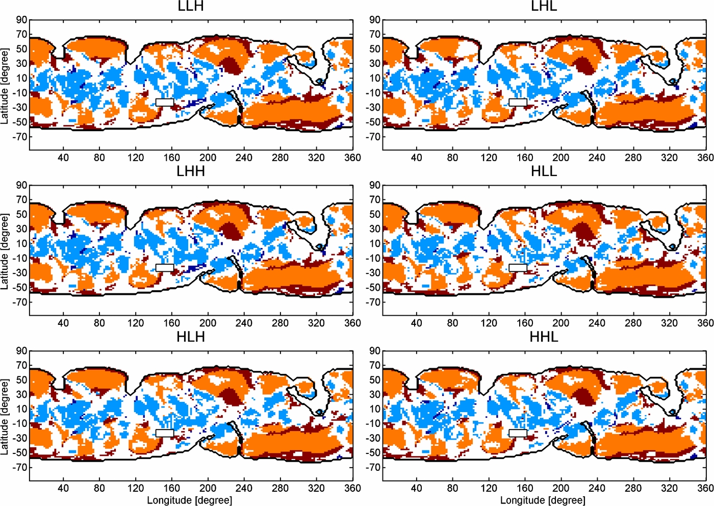
Figure 9 is similar to Figure 2, except that it shows how the spatial distribution of the up and down loops differs according to the location in the error box. While some differences can be noted, none of these changes exhibit obvious systematic trends, so the overall pattern does not change. Figure 10 is similar to Figure 8, but instead it shows the results from the corners of the error boxes. While the derived temperature change, the gradient directions do not, so all corners of the error box show consistency with the up/down loop interpretation.
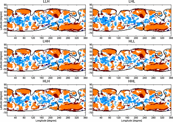
Figure 9. Similar to Figure 2, except each image represents one corner of the error box, as indicated. Note that the spatial distribution of the up and down loops changes very little.
Download figure:
Standard image High-resolution image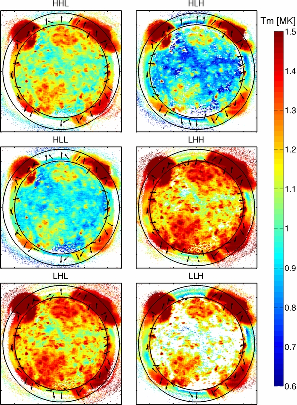
Figure 10. Similar to Figure 8, except each image represents one corner of the error box, as indicated. Note that the spatial distribution of the gradient arrows changes very little.
Download figure:
Standard image High-resolution image
Footnotes
- 3
- 4
The most optically thick part of an image of the solar corona corresponds to an LOS that just grazes the limb. Lines of sight hitting disk terminate at 1.0 R☉, while those grazing the limb pass through more plasma. (We call this the black ball model in which the effect of the chromosphere is to terminate the LOS but not contribute to the optical depth.) Thus, the tomography algorithm makes use of LOSs that hit the center of the disk as well as those above 1.025 R☉, and it only ignores the image data between 0.98 and 1.025 R☉. The effect of ignoring this data makes part of the tomographic matrix ill-conditioned, resulting in unreliable emissivities in the radial range between about 1.0 and 1.03 R☉ (Frazin et al. 2009).
- 5
A "loop" is deemed to consist of two "legs," each ascending from a foot-point to the loop's apex.
- 6
R2 ≡ 1 − Sres/Stot, where Sres is the sum of the squared residuals and Stot is the sum of data's deviations from the mean.
- 7
The early mission data allow the STEREO-A/171 and STEREO-B/171 to be scaled so that they have effectively the same radiometric calibration. The same applies to the other wavelengths.