


ABSTRACT
We study the fluence distributions of over 3040 bursts from SGR 1806−20 and over 1963 bursts from SGR 1900+14 using the complete set of observations available from the Rossi X-Ray Timing Explorer/Proportional Counter Array through 2011 March. Cumulative event distributions are presented for both sources and are fitted with single and broken power laws as well as an exponential cutoff. The distributions are best fitted by a broken power law with exponential cutoff; however the statistical significance of the cutoff is not high and the upper portion of the broken power law can be explained as the expected number of false bursts due to random noise fluctuations. Event distributions are also examined in high and low burst rate regimes and power-law indices are found to be consistent, independent of the burst rate. The contribution function of the event fluence is calculated. This distribution shows that the energy released in the soft gamma repeater (SGR) bursts is dominated by the most powerful events for both sources. The power-law nature of these distributions combined with the dominant energy dissipation of the system occurring in the large, less frequent bursts is indicative of a self-organized critical system, as suggested by Goğus et al. in 1999.
Export citation and abstract BibTeX RIS
1. INTRODUCTION
Soft gamma repeaters (SGRs) are associated with slowly rotating, extremely magnetized neutron stars (NSs; see reviews by Woods & Thompson 2006; Mereghetti 2008). They are sometimes found in young supernova remnants and are characterized by recurrent emission of short duration, ∼0.1 s (Kouveliotou 1995), bursts of soft gamma-rays/hard X-rays with spectra described by optically thin thermal bremsstrahlung (OTTB) at kT ∼ 20–40 keV (Goğus et al. 2001). Recent studies at lower energies, <15 keV, have found that an OTTB model is no longer accurately fitted to the spectra and there is a rollover which can be best fitted with two blackbodies or alternatively a cutoff power law (Feroci et al. 2004; Olive et al. 2004; Nakagawa et al. 2007; Israel et al. 2008; Lin et al. 2011; van der Horst et al. 2012). There is evidence that these bursts are the result of starquakes that occur when the NS crust fractures due to a buildup of stress associated with the evolution of the strong magnetic field, greater than 1014 G (Thompson & Duncan 1995).
In Thompson & Duncan's seminal 1995 paper first describing magnetars they give a theoretical description of the repeating bursts observed from SGRs. The ultra-strong magnetic fields rotating with the core of the NS are pulled through the crust, causing stress to build up. When the stresses become more than the crust can support it fractures. An electron/positron pair plasma is ejected from the star and captured by the magnetic field near the NS surface. This plasma then cools via emission of soft gamma rays and X-rays.
The statistical properties of SGR bursts have been shown to be similar to those observed for earthquakes (Cheng et al. 1996; Gutenberg & Richter 1956, 1965). Event energy distributions from SGR 1806−20 and SGR 1900+14 sources have been well fitted with a power law described by dN ∝ E−γ dE and an exponent, γ, of 1.6–1.7 (Goğus et al. 1999, 2000). Many natural systems have been found to fit power laws (Aschwanden 2011). This power-law distribution of energy release was recognized to occur in many natural systems that exhibit nonlinear energy dissipation and is commonly referred to as a self-organized critical (SOC) system (Bak et al. 1987).
Here, we report on burst energy distributions using all of the data available from the Rossi X-ray Timing Explorer (RXTE) for two of the most active SGRs, SGR 1806−20 and SGR 1900+14, covering the period from 1996 December to 2011 February. The initial search found 3040 bursts from SGR 1806−20 and 1963 from SGR 1900+14. Differential and cumulative event fluence distributions are presented for each source. These were fitted with single power laws as reported by past authors (Laros et al. 1987; Woods et al. 1999; Goğus et al. 1999), but we also fitted single and broken power laws with exponential cutoffs and were able to improve upon the quality of fit for each source. We also use the large number of bursts observed to define periods of high and low burst activity. The burst fluence distribution for high and low burst phases was then analyzed. The contribution function was calculated for the burst fluence distributions. This function would be peaked at a characteristic fluence if one existed in the data set. This distribution shows the contribution of the different fluence bins to the total energy released by the bursts. In Section 2 the observations for each source are described, Section 3 covers analysis and the results, and Section 4 presents our conclusions.
2. TARGETS AND OBSERVATIONS
SGR 1806−20 has been observed to exhibit sporadic bursting behavior since 1983 (Laros et al. 1987). The Burst and Transient Source Experiment (BATSE) onboard the Compton Gamma-Ray Observatory launched in (April 1991) detected more sporadic bursting behavior. It entered an active phase in 1996. Two weeks of observations with RXTE/PCA led to the discovery of 7.47 s pulsations and confirmed its nature as a magnetar (Kouveliotou et al. 1998). This source remained relatively inactive until it released a giant flare in 2004 (Hurley et al. 2005). The luminosity of this flare had a peak of a few times 1047 erg s−1 (Hurley et al. 2005; Palmer et al. 2005). The source remained active, emitting hundreds of smaller bursts for the next two years, although it generally decreased in activity over that time.
SGR 1900+14 became active in 1998 May after a period of long inactivity (Kouveliotou et al. 1993). It then emitted a giant flare in 1998 August (Hurley et al. 1999). The persistent emission from this source shows pulsations with a period of 5.2 s, matching the period of pulsations observed in the tail of the 1998 giant flare (Cline et al. 1998; Hurley 1999; Feroci 2001). The source has remained active over the last decade but no further giant flares have been observed.
The PCA on board RXTE observed SGR 1806−20 and SGR 1900+14 for a total of more than 800 hr, or 3 Ms, each. An automated burst search, similar to the searches by Woods et al. (1999) and Goğus et al. (1999), was performed for all of the available data. We used standard-1 (2–60 keV) data constrained to observations 5° above Earth's horizon. Each 0.125 s bin was searched. A background count rate was estimated using 5 s of data 3 s before and after the bin being searched. Bins in excess of 125 counts bin−1 were assumed to contain burst emission and were excluded from the background estimate. A burst was defined as any continuous set of bins in which the count rate exceeded 5.5σ the average local background rate. The count fluence was then estimated by integrating the background-subtracted counts for all bins included in the burst. Bursts which happen very close in time were counted as a single burst if their fluence did not drop below the 5.5σ of the average local background rate and counted as multiple bursts when they did. There were a small number of bursts which saturated the RXTE/PCA and were left out of our study because the burst fluence cannot be accurately calculated for these events. We report the fluence in PCA counts PCU−1 because no spectral analysis was done in this work. A conversion factor, 2 × 10⁻¹² erg cm−2 counts−1, can be used to determine the burst fluence in erg cm−2. This was reported by Goğus et al. (1999, 2000) based on BATSE spectral measurements.
3. ANALYSIS AND DISCUSSION
We fitted the data for each source using differential and cumulative distributions. The data were initially fitted with a single power law but for both types of distribution the fit parameters indicated that the likelihood of the model representing the data was very low, with reduced χ2 values between 3 and 5 and a Kolmogorov–Smirnov (K-S) probability of zero for both sources. Examining the fluence distributions of each source (Figures 1 and 2), it is apparent that at the lower and upper ends of the distribution there are more components to the fit. We then fitted a broken power law and exponential cutoff using the cumulative distributions. The cumulative distribution retains all of the original information from the data set and more clearly shows the excess and falloff from the power law. The method and results for each source, distribution, and different fits are described in the following section.
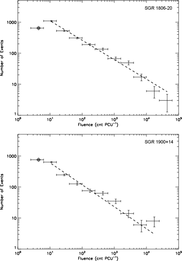
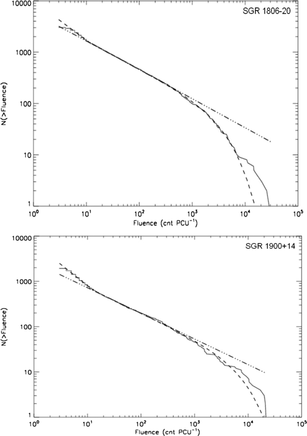
Figure 1. Differential burst fluence distributions for SGR 1806−20 (top) and SGR 1900+14 (bottom). Both are well fitted by a power law of the form dN ∝ E−γ dE, with γ = 0.63 ± 0.04 for SGR 1806−20 and 1.71 ± 0.06 for SGR 1900+14. The lowest fluence bin was excluded from the fit due to decreased detector sensitivity and increased sensitivity to background fluctuations. Download figure: Figure 2. Solid line is data, dash-dotted is a single power law N (>E) ∝ E1−γ and the dashed is a broken power law plus exponential cutoff, E1−γ eαx. The exponential cutoff is, however, not significant and the high-fluence falloff is likely from a poor sampling of the upper fluence events. The excess at low fluence, fitted by the upper power law, corresponds to the number of expected false detections of bursts during the 3 Ms of observations for each source, Section 3.2. The fits are consistent with a single power law over three orders of magnitude, a fingerprint of self-organized critical (SOC) behavior. Download figure:
3.1. Differential Distributions of Burst Fluence
The events from each data set were binned in equally spaced logarithmic fluence steps (dN/d log E). The number of bins for each distribution was determined by using the Sturges formula (Sturges 1926), given by log2 N+1 where N is the number of events in the distribution. Using a least-squares fitting method, the data are well fitted by a power-law distribution over three orders of magnitude in fluence. The power-law exponent, γ, was found to be 0.63 ± 0.04 for SGR 1806−20 and 0.71 ± 0.06 for SGR 1900+14 where dN ∝ E−γ dE, see Figure 1. The exponent depends strongly on where the lower threshold was set for thresholds near the minimum detectable fluence but, as mentioned above, none of the single power-law fits shows evidence of being a good fit to the data with reduced χ2 values between 3 and 5. We excluded the first point in the distribution, shown as a diamond, as this represents events only a few counts above the threshold and thus in the limited sensitivity range of the detector.
The differential distribution for SGR 1806−20 shows a dropoff below the single power law in the highest fluence bins. We attempted to fit a broken power law and single power law with exponential cutoff to account for this feature but neither provides a significantly improved fit due to the low statistics at the high fluence end of the distribution. The inability to fit this feature as well as the lowest data bin included in the fit motivated our use of the cumulative distribution described in Section 3.2. The values for a single power-law fit to the differential distribution are consistent with those reported by Goğus et al. (1999, 2000).
3.2. Cumulative Distributions of Burst Fluence
Cumulative distributions were calculated and fitted with a single power law using the maximum likelihood method. The uncertainty in the cumulative distribution was determined from the Poisson uncertainty in the binned data, resulting in using the square root of the sum of all the counts greater than a given fluence. The differential power law described in Section 3.1 is related to that fitted to the cumulative distribution by the following, N (>E) ∝ E1−γ. The single power-law fit to the cumulative distribution above a low fluence cutoff of 5 counts PCU−1, as described above being due to low detector sensitivity, has K-S probabilities of zero. Examining the cumulative distribution, Figure 2, the large excess at low fluence and dropoff at high fluence clearly stand out. Fitting a broken power law for both sources dramatically improves the quality of fit, with K-S probabilities of 0.999 for SGR 1806−20 and 0.945 for SGR 1900+14. For SGR 1806−20 γ = 1.54 ± 0.01 and for SGR 1900+14 γ = 1.56 ± 0.02. Adding an exponential cutoff to account for the high fluence dropoff, N (>E) ∝ E1−γexp(αE), failed to improve the quality of the fit significantly. Each fit, with and without the exponential cutoff, has the same K-S probability out to five significant figures. Figure 2 shows multiple fits to the cumulative distribution for each source and Table 1 gives fit parameters and goodness-of-fit results for each source and model.
Table 1. Fit Parameters and Quality of Fit for Cumulative SGR Burst Fluence Distributions
| Fit Parameters | ||||||
|---|---|---|---|---|---|---|
| SGR 1806−20 | γ1 | γ2 | Break (counts PCU−1) | α | K-S | K-S Probability |
| All Bursts 3040 bursts | ||||||
| Single power law | ... | 1.58 ± 0.03 | ... | ... | 0.086 | 0.000 |
| Broken power law | 1.77 ± 0.01 | 1.54 ± 0.01 | 12 | ... | 0.007 | 0.999 |
| Broken power law with exponential cutoff | 1.77 ± 0.01 | 1.54 ± 0.01 | 12 | −2.2 ± 0.47 × 10⁻⁴ | 0.007 | 0.999 |
| High Burst Rate 2232 bursts | ||||||
| Single power law | ... | 1.59 ± 0.03 | ... | ... | 0.070 | 0.000 |
| Broken power law | 1.75 ± 0.01 | 1.56 ± 0.01 | 12 | ... | 0.008 | 0.999 |
| Broken power law with exponential cutoff | 1.75 ± 0.01 | 1.56 ± 0.01 | 12 | −2.4 ± 0.59 × 10⁻⁴ | 0.008 | 0.999 |
| Low Burst Rate 323 bursts | ||||||
| Single power law | ... | 1.59 ± 0.03 | ... | ... | 0.188 | 0.000 |
| Broken power law | 2.42 ± 0.04 | 1.59 ± 0.02 | 8 | ... | 0.013 | 0.999 |
| Broken power law with exponential cutoff | 2.42 ± 0.04 | 1.59 ± 0.02 | 8 | −1.0 ± 0.41 × 10⁻⁴ | 0.013 | 0.999 |
| SGR 1900+14 | ||||||
| All Bursts 1963 bursts | ||||||
| Single power law | ... | 1.64 ± 0.04 | ... | ... | 0.152 | 0.000 |
| Broken power law | 1.94 ± 0.03 | 1.56 ± 0.02 | 14 | ... | 0.014 | 0.945 |
| Broken power law with exponential cutoff | 1.94 ± 0.03 | 1.56 ± 0.02 | 14 | −1.2 ± 0.10 × 10⁻⁴ | 0.014 | 0.945 |
| High Burst Rate 1626 bursts | ||||||
| Single power law | ... | 1.63 ± 0.04 | ... | ... | 0.126 | 0.000 |
| Broken power law | 1.85 ± 0.03 | 1.55 ± 0.02 | 14 | ... | 0.015 | 0.971 |
| Broken power law with exponential cutoff | 1.85 ± 0.03 | 1.55 ± 0.02 | 14 | −1.7 ± 0.11 × 10⁻⁴ | 0.016 | 0.951 |
| Low Burst Rate 236 bursts | ||||||
| Single power law | ... | 1.73 ± 0.04 | ... | ... | 0.273 | 0.000 |
| Broken power law | 2.48 ± 0.04 | 1.57 ± 0.02 | 10 | ... | 0.019 | 0.999 |
| Broken power law with exponential cutoff | 2.48 ± 0.04 | 1.57 ± 0.02 | 10 | −8.5 ± 1.6 × 10⁻⁴ | 0.019 | 0.999 |
Notes. Multiple models were fitted for each source distribution including a single power law (N (>E) ∝ E1−γ2), broken power law (E < Break: N (>E) ∝ E1−γ1 and E ⩾ Break: N (>E) ∝ E1−γ2), and broken power law with exponential cutoff, where the power law above the break is multiplied by exp(αE).
Download table as: ASCIITypeset image
The need for a lower fluence power law in addition to the power law covering the middle three orders of magnitude in the distribution is due to the large excess above a single power-law fit to the other three orders of magnitude. The power law at lower fluence has γ = 1.77 ± 0.01 for SGR 1806−20 and γ = 1.94 ± 0.03 for SGR 1900+14. Assuming the detector noise fits a Poisson distribution we estimate that for 3 Ms of observing time with 0.125 s bins there should be ∼360 false bursts detected due to noise fluctuations above the 5 counts PCU−1 cutoff. This is on the order of the excess in bursts observed for each source which have different numbers of bursts but almost the same amount of observing time. Fitting a high burst rate and low burst rate distribution, as described in Section 3.4, gives more support to this explanation for the low fluence excess. The low burst rate distribution, which contains very few bursts but the majority of the observing time, is seen to have most of the excess events, Figure 5.
The falloff at high fluence which appears visually in the cumulative distribution of each source, although more exaggerated for SGR 1806−20, can be fitted with the inclusion of an exponential cutoff with α = −2.2 ± 0.47 × 10⁻⁴ for SGR 1806−20 and α = −1.2 ± 0.10 × 10⁻⁴ for SGR 1900+14. However, the goodness of fit remains unchanged because the K-S value is dominated by the largest difference between model and data, which occurs at a lower fluence where the power-law fit dominates.3 Goğus et al. (1999, 2000) exclude the high fluence events from their fits with the argument that the intrinsic distribution is under-sampled. The visual fit with the exponential component appears better than the fit without, suggesting that the dropoff in high fluence events is real; however the low statistics do not allow this to be determined definitively. If the dropoff is related to a characteristic fluence at approximately 30,000 counts PCU−1, it may be difficult to confirm until there are significantly more events due to the low statistics at higher fluence.
3.3. Contribution Function Distribution
To better understand the nature of these events and how the energy release is distributed, we examined the contribution function, (dN/d log E) E, for the fluence distributions. Using the differential distribution we calculated the contribution function and plotted it against d log E. This distribution should peak at the characteristic fluence of the intrinsic distribution, see Figure 3. Instead we observe a distribution well fitted by a single power law over four orders of magnitude, with exponents of 1.37 ± 0.03 and 1.34 ± 0.05 for SGR 1806−20 and SGR 1900+14, respectively. This further supports the idea that the falloff observed in the cumulative fluence distribution is not related to the characteristic fluence of the sources. Both distributions indicate that the largest portion of energy release occurs in the highest fluence bursts instead of the more numerous low fluence bursts.
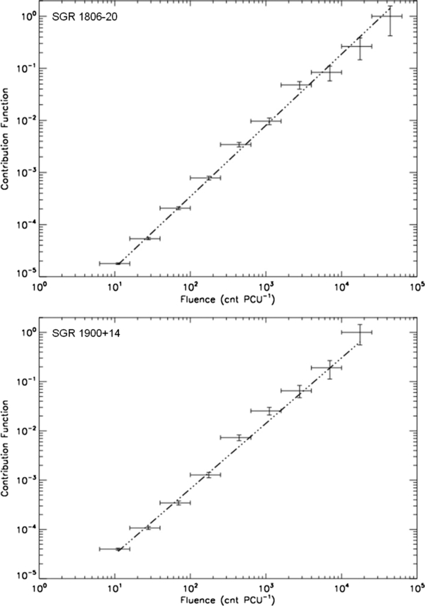
Figure 3. Fluence distribution was binned and the contribution function, (dN/d log E) E, was calculated. The distribution is well fitted by a single power law over four orders of magnitude and shows that while the highest fluence bursts occur least often, they dominate the energy release in the system, another sign of SOC behavior. The normalized contribution is shown.
Download figure:
Standard image High-resolution image3.4. Event Distributions as a Function of Burst Activity
The large number of detected bursts allows us to distinguish between different levels of burst activity for each source. Figure 4 shows the burst rate for all observations of each source. We define high burst activity as a burst rate exceeding the average rate for all observations, approximately 1 burst ks−1 of observing time for each source. Cumulative fluence distributions were made for separate periods of burst activity for each source and fitted with a single power law and a broken power law with exponential cutoff as described in Section 3.2. The burst-rate-dependent cumulative distributions are shown in Figure 5. The exponents for each source are the following: SGR 1806−20 high phase is 1.56 ± 0.02 and low phase is 1.59 ± 0.03; SGR 1900+14 high phase is 1.55 ± 0.02 and low phase is 1.57 ± 0.02. The fit parameters and goodness-of-fit values are summarized in Table 1. The power-law exponent for each phase is consistent with that of the total bursts indicating that the burst fluence statistics are independent of the level of burst activity over the time for which we have observations with RXTE/PCA, approximately 15 years. The fact that the excess of events at low fluence is dominant in the low burst rate regime is supportive of the idea that this excess is due to random fluctuations in the background, as suggested in Section 3.2.
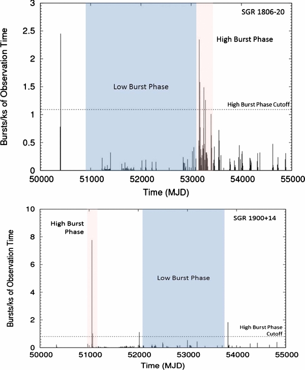
Figure 4. Number of bursts per ks of observation over 3 Ms of observations for SGR 1806−20 (top) and SGR 1900+14 (bottom). The high burst activity is defined as any observation where the burst rate exceeds that average rate for all of the observations, approximately 1 burst ks−1 for each source. Fluence distributions were made for each phase, shown in the shaded regions, and are presented in Figure 5
Download figure:
Standard image High-resolution image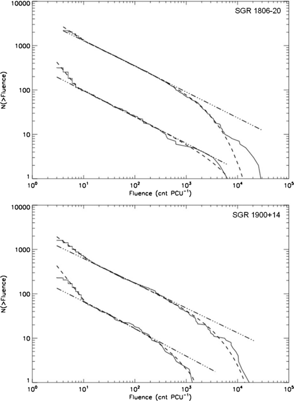
Figure 5. Cumulative distributions for low (bottom curve) and high (upper curve) rates of burst activity fitted with single power law, N (>E) ∝ E1−γ, and broken power law with exponential cutoff, E1−γ eαx. The fits are consistent with those calculated for the entire distribution. The event fluence is thus independent of the rate of bursts, an important fingerprint of self-organized critical (SOC) behavior. Table 1 gives the fit parameters and the number of bursts included for each source and model.
Download figure:
Standard image High-resolution image4. CONCLUSIONS
The collected RXTE/PCA observations for SGR 1806−20 and SGR 1900+14 provide thousands of bursts for each source to perform statistical analysis on the fluence distributions. We fitted the cumulative distributions for SGR 1806−20 and SGR 1900+14 with a single power law, broken power law, and both with exponential cutoffs. The distributions were best fitted with a broken power law with exponential cutoff but there is not a significant statistical difference between that and the broken power law without a cutoff. Fitting all the features of the distribution allowed us to improve the uncertainty on the fit parameters for a single power law over three orders of magnitude, giving γ = 1.54 ± 0.01 and γ = 1.56 ± 0.02 for SGR 1806−20 and SGR 1900+14, respectively.
The contribution function was calculated for each source and was found to be well fitted by a single power law over four orders of magnitudes of fluence. The function is clearly not peaked; thus we do not observe a characteristic fluence in these distributions. It also shows how energy release in repeating bursts is dominated by the emission from high fluence events instead of the more numerous low fluence events.
The burst activity for each source varies significantly over the ∼3 Ms of observations. We found the power-law fits for data at high and low burst rate and find that the exponents for different levels of activity are consistent with the exponent for the total event distribution. This indicates that the fluence of individual bursts is independent of burst activity; however the rate of bursts can vary significantly over time.
The power-law fits to the event fluence distributions when all the events are included as well as the rate-dependent distributions, especially when considered over three orders of magnitude, provide strong evidence that the repeating bursts from SGRs are the result of an SOC system. The independence of the power-law fit from burst rate is another indicator of SOC behavior. An SOC system requires a constant source of energy; in SGRs this can be attributed to the ultra-strong magnetic fields. The undoubtedly complex nature of the interactions occurring in the crust of an NS combined with this constant source of power in the magnetic field then explains why we observe SOC behavior from SGRs.
We thank Ken Gayley for his suggestion to calculate the contribution function and for his help in doing so. We also thank Joanne Hill, Randall McEntaffer, and Craig Kletzing for their comments. Fotis Gavriil also offered important advice for this work.
Footnotes
- 3
The K-S value is defined as the maximum value of the absolute difference between two cumulative distributions and appears as follows:
 (Press et al. 1989).
