


ABSTRACT
Using Hubble Space Telescope observations of 147 host galaxies of low-mass black holes (BHs), we systematically study the structures and scaling relations of these active galaxies. Our sample is selected to have central BHs with virial masses of ∼105–106 M☉. The host galaxies have total I-band magnitudes of −23.2 < MI < −18.8 mag and bulge magnitudes of −22.9 < MI < −16.1 mag. Detailed bulge–disk–bar decompositions with GALFIT show that 93% of the galaxies have extended disks, 39% have bars, and 5% have no bulges at all at the limits of our observations. Based on the Sérsic index and bulge-to-total ratio, we conclude that the majority of the galaxies with disks are likely to contain pseudobulges and very few of these low-mass BHs live in classical bulges. The fundamental plane of our sample is offset from classical bulges and ellipticals in a way that is consistent with the scaling relations of pseudobulges. The sample has smaller velocity dispersion at fixed luminosity in the Faber–Jackson plane compared with classical bulges and elliptical galaxies. The galaxies without disks are structurally more similar to spheroidals than to classical bulges according to their positions in the fundamental plane, especially the Faber–Jackson projection. Overall, we suggest that BHs with mass ≲ 106 M☉ live in galaxies that have evolved secularly over the majority of their history. A classical bulge is not a prerequisite to host a BH.
Export citation and abstract BibTeX RIS
1. INTRODUCTION
In the past decade, we have found strong correlations between supermassive black hole (BH) masses (∼106–109 M☉) and the properties of host bulges (e.g., the MBH–σ* relation; Tremaine et al. 2002, and the MBH–Lbulge relation; Marconi & Hunt 2003). However, very little is known about BH–bulge correlations for low-mass BHs (<106 M☉) or late-type galaxies. The correlations between BH mass and galaxy properties in this low-mass regime provide important constraints on the formation mechanisms of the first primordial seed BHs (e.g., Volonteri & Natarajan 2009). Furthermore, low-mass BHs are expected to be a major source of gravitational radiation (e.g., Hughes 2002). Given the strong correlations between bulge properties and BH mass, the question remains whether supermassive BHs can exist in bulgeless galaxies, and if so how massive they become.
It was originally thought that BH mass was linked exclusively with bulge mass. For instance, the nearby late-type spiral galaxy M33 does not contain a central BH more massive than 1500 M☉ (e.g., Gebhardt et al. 2001; Merritt et al. 2001). Similarly, a central BH in the nearby dwarf galaxy NGC 205 has an upper limit of 2.2 × 10⁴ M☉ on its mass (e.g., Valluri et al. 2005). On the other hand, recent observations show that central massive BHs can also exist without classical bulges (e.g., Filippenko & Ho 2003; Greene & Ho 2004, 2007b; Barth et al. 2004, 2009; Satyapal et al. 2007, 2009; Shields et al. 2008). Prior to our work, NGC 4395 and POX 52 were the only galaxies known to host BHs with MBH ≲ 106 M☉. NGC 4395 is an Sdm spiral with no bulge. POX 52 is a spheroidal galaxy, also sometimes called a dwarf elliptical, although we follow the naming convention of Kormendy et al. (2009). One has a disk, and the other has no disk. Neither has a classical bulge component. A larger sample of low-mass BHs is needed to understand the properties of their host galaxies.
Finding low-mass BHs is particularly challenging. Unlike massive BHs in nearby galaxies, it is nearly impossible to measure dynamical BH masses for BHs with ≲ 106 M☉ outside of the Local Group. We cannot yet resolve their gravitational spheres of influence, although it is possible to place interesting constraints on central BH masses in nearby objects (e.g., Barth et al. 2009; Seth et al. 2010). Instead, we rely on indirect methods to estimate the "virial" masses of actively accreting BHs. Based on the broad Hα profile and the calibrated radius–luminosity relation (e.g., Bentz et al. 2009b), Greene & Ho (2004) presented 19 galaxies with virial BH masses ≲ 106 M☉. The sample has since increased to 174 galaxies (Greene & Ho 2007b; see also Dong et al. 2007). From the Sloan Digital Sky Survey (SDSS) data alone, we do not learn much about the host galaxy properties. Here, we present a study of the host galaxies of this large sample of low-mass BHs using Hubble Space Telescope (HST) observations. Our primary goal is to determine the morphological types of galaxies hosting low-mass BHs, in particular the types of bulges that they contain. From the SDSS images, we know that the galaxies are ∼1 mag below L* (Greene & Ho 2004). In this luminosity range, galaxies have many different morphologies, ranging from small elliptical galaxies (e.g., M32) to late-type spirals and spheroidals. We want to determine whether a bulge is a necessary requirement to host a central supermassive BH.
First, we will measure the fraction of low-mass BHs without a bulge-like component of any kind. Bulgeless galaxies observed in the nearby universe, such as NGC 4395 and NGC 6946 (e.g., Filippenko & Ho 2003; Shih et al. 2003; Boomsma et al. 2008), are recognized as a challenge to the cold dark matter galaxy formation scenario (e.g., Kormendy & Fisher 2008; Kormendy et al. 2010; Peebles & Nusser 2010). The fact that there are BHs in bulgeless galaxies implies that a bulge is not a necessary condition for the formation of BHs. Satyapal et al. (2009) study 18 truly bulgeless Sd/Sdm galaxies with Spitzer and find only one active galaxy (NGC 4178), which suggests that BHs in bulgeless galaxies may be truly rare. X-ray observations find active galactic nuclei (AGNs) in ∼25% of Scd–Sm galaxies (Desroches & Ho 2009). Larger samples of such bulgeless host galaxies will elucidate their nature.
Second, we will determine what fraction of the low-mass BH hosts have no disk. These may be either elliptical or spheroidal galaxies (e.g., Ferrarese et al. 2006; Kormendy et al. 2009). More massive BHs are found in elliptical galaxies, but these lower-mass systems have stellar masses that are consistent with being either small ellipticals or spheroidals. We will use their scaling relations (e.g., the fundamental plane) to distinguish between these two types. The differing structures of spheroidal and elliptical galaxies likely reflects different formation histories (e.g., Kormendy et al. 2009), and so the question is whether BH formation and growth occurs in spheroidal systems.
Third, for the disk galaxies with a bulge component, we ask whether or not they are classical bulges. Observational evidence is building that there are two different kinds of bulges, namely, classical bulges and pseudobulges (e.g., Kormendy & Kennicutt 2004). Pseudobulges have properties, including rotational support, exponential profiles, and ongoing star formation, that implicate the importance of secular processes such as bar transport in their buildup. We will measure the structure of the bulges from the HST observations to decide whether they are pseudobulges or classical bulges.
Finally, many recent papers have hinted that the scaling relations between low-mass BHs and their bulges are systematically different compared with more massive BHs (e.g., Hu 2008; Greene et al. 2008, 2010; Gadotti & Kauffmann 2009). Ultimately, we will use the structural measurements presented here to examine the MBH–Lbulge and MBH–Mbulge correlations for this sample (Jiang et al. 2011).
In Section 2, we describe the data and reduction process. In Section 3, we present the image decompositions. We explain how the uncertainties and upper limits are estimated in Section 4. Morphological results are given in Section 5 and scaling relations are given in Section 6. Finally, in Section 7, we summarize the paper. The following cosmological parameters have been adopted: H0 = 100h = 71 km s−1 Mpc−1, Ωm = 0.27, and ΩΛ = 0.75 (Spergel et al. 2003). Galactic extinction is calculated based on the fitting formula given by Cardelli et al. (1989).
2. THE DATA
In this section, we first briefly present the sample selection. We then describe the data reduction processes used to produce the final images for analysis.
2.1. Our Sample
The galaxies presented here are drawn from the sample described in Greene & Ho (2007b). This sample is selected from all broad-line active galaxies in the Fourth Data Release (DR4; Adelman-McCarthy et al. 2006) of the SDSS (e.g., York et al. 2000; Greene & Ho 2007a) with z < 0.35. First, the DR4 spectra are continuum-subtracted using a principal component analysis developed by Hao et al. (2005). Then objects with high rms deviations above the continuum in the broad Hα region are selected, and a more detailed profile fitting is applied to isolate those objects with Hα profiles that are broad compared to the narrow [S ii] and [N ii] lines.
Virial BH masses are estimated for all targets, using the broad-line region (BLR) gas as the dynamical tracer. The virial mass is simply MBH = fR(Δv)2/G, where R is the size of the BLR, Δv is a measure of the broad-line width, such as FWHM, and f is a dimensionless factor that accounts for the unknown geometry and kinematics of the BLR. A few dozen AGNs have direct measurements of their BLR sizes from reverberation mapping, a measurement of the lag between continuum and line variations (e.g., Peterson et al. 2004; Bentz et al. 2009b; Denney et al. 2010). An empirical correlation between BLR radius and AGN luminosity (the radius–luminosity relation) is then used to infer the BLR sizes for other AGNs (e.g., Bentz et al. 2006, 2009b). In this work, we use the luminosity of Hα to infer the BLR radius (Greene & Ho 2005b). The virial mass is then estimated from the luminosity and FWHM of Hα as (e.g., Greene & Ho 2007b; Woo et al. 2010)
Since we cannot yet determine the value of f for each AGN appropriately, we use a single value of f = 0.75 (e.g., Kaspi et al. 2000) that is intended to represent an ensemble average over our sample. The virial masses we use in this paper are calculated according to the above formula with the Hα luminosity and FWHM based either on the SDSS spectrum or a higher-resolution spectrum from the Echelle Spectrograph and Imager (ESI) on Keck (Sheinis et al. 2002) or the Magellan Echellette Spectrograph (MagE; Marshall et al. 2008). The spectra are presented in Xiao et al. (2011).
From this parent sample, the final 174 BHs were selected to have virial masses smaller5 than 2 × 10⁶ M☉ (Greene & Ho 2007b). An additional 55 galaxies were presented with far-less-certain broad-line masses (called "c"). The HST snapshot pool was taken from these 229 galaxies. These galaxies have a median g-band magnitude of Mg = −19.3 and a median color of 〈g − r〉 = 0.7 mag. The median redshift is 〈z〉 = 0.085, with a maximum redshift of z = 0.35. They have BHs with virial masses ranging from MBH = 6.2 × 10⁴ M☉ to 3.8 × 10⁷ M☉ with a median value 1.2 × 10⁶ M☉. The BHs are radiating at high fractions of their Eddington limits and most are radio quiet. More properties of these galaxies are described in Greene & Ho (2007b).
2.2. Observations
In order to study the detailed structure of the host galaxies, we were awarded a snapshot survey with WFPC2 on HST in cycle 16. A total of 147 galaxies from Greene & Ho (2007b) were observed during this program, including some from the "c" sample. Each galaxy was placed at the center of the Planetary Camera CCD. The WFPC2 field of view is divided into four cameras by a four-faceted pyramid mirror near the HST focal plane.6 Each camera contains an 800 × 800 pixel detector. Three identical cameras, with a plate scale of 0 1 pixel−1, form an "L" shape. The fourth camera, the Planetary Camera, is located at the upper right corner of the "L" and has a finer plate scale of 0046 pixel−1. The total effective field of view is ∼322 × 322. The typical FWHM of the point-spread function (PSF) for the Planetary Camera is ∼1.7 pixels in the F814W filter.
Details of the observations are summarized in Table 1. For each object we obtained a short (30 s) exposure in the case of saturation, followed by two dithered ∼600 s exposures with the F814W filter. The mean wavelength of this filter is 8269 Å and the central wavelength is 8012 Å, which is a little different from the Johnson I-band filter. As discussed in Greene et al. (2008), independent of galaxy color the difference in magnitude between F814W and I is so small (<0.05 mag) that throughout we will refer to the HST observations as I-band images.
Table 1. Observations Summary
| Name | SDSS Name | z | AI | Observation Date | Scale | log MBH |
|---|---|---|---|---|---|---|
| (mag) | (arcsec kpc−1) | (M☉) | ||||
| (1) | (2) | (3) | (4) | (5) | (6) | (7) |
| 0022−0058 | SDSSJ002228.36−005830.6 | 0.106 | 0.32 | 2008 Aug 22 | 0.42 | 5.7 |
| 0024−1038 | SDSSJ002452.53−103819.6 | 0.103 | 0.15 | 2008 Sep 25 | 0.43 | 6.2 |
| 0117−1001 | SDSSJ011749.81−100114.5 | 0.141 | 0.50 | 2008 Aug 19 | 0.31 | 5.8 |
| 0120−0849 | SDSSJ012055.92−084945.4 | 0.125 | 0.14 | 2008 Jun 9 | 0.35 | 6.3 |
| 0158−0052 | SDSSJ015804.75−005221.8 | 0.0804 | 0.05 | 2008 Sep 27 | 0.56 | 5.9 |
| 0228−0901 | SDSSJ022849.51−090153.7 | 0.0722 | 0.13 | 2007 Oct 22 | 0.63 | 5.4 |
| 0233−0748 | SDSSJ023310.79−074813.3 | 0.0310 | 0.20 | 2008 Nov 1 | 1.52 | 6.0 |
| 0240+0103 | SDSSJ024009.10+010334.5 | 0.196 | 0.038 | 2007 Nov 19 | 0.22 | 5.8 |
| 0304+0028 | SDSSJ030417.78+002827.3 | 0.0444 | 0.071 | 2008 Sep 23 | 1.05 | 6.1 |
| 0325+0034 | SDSSJ032515.59+003408.4 | 0.102 | 0.071 | 2008 Nov 25 | 0.44 | 6.0 |
| 0327−0756 | SDSSJ032707.32−075639.3 | 0.154 | 0.15 | 2008 Dec 5 | 0.28 | 5.7 |
| 0347+0057 | SDSSJ034745.41+005737.2 | 0.179 | 0.061 | 2008 Jul 27 | 0.24 | 7.6 |
| 0731+3926 | SDSSJ073106.86+392644.6 | 0.0483 | 0.057 | 2008 Nov 22 | 0.96 | 6.1 |
| 0735+4235 | SDSSJ073505.65+423545.6 | 0.0858 | 0.041 | 2008 Sep 9 | 0.53 | 6.2 |
| 0744+2430 | SDSSJ074423.44+243046.3 | 0.117 | 0.072 | 2008 Nov 13 | 0.38 | 6.2 |
| 0748+4540 | SDSSJ074810.36+454003.1 | 0.143 | 0.15 | 2008 Nov 17 | 0.30 | 6.3 |
| 0748+4052 | SDSSJ074825.27+405217.8 | 0.136 | 0.37 | 2008 Nov 23 | 0.32 | 5.7 |
Notes. Column 1: abridged SDSS name. Column 2: full SDSS name as well as coordinates. Column 3: galaxy redshift. Column 4: galactic extinction in the I band. Column 5: date of observation. Column 6: physical scale of image. Column 7: virial BH mass.
Only a portion of this table is shown here to demonstrate its form and content. A machine-readable version of the full table is available.
Download table as: DataTypeset image
2.3. Data Reduction
The raw HST data must be processed before they can be used for scientific analysis. Since the short exposure is only used in two cases (described at the end of this section), we focus here on the long exposures.
The first step is to remove cosmic rays (CRs) using the identification script LACosmic (van Dokkum 2001), which can detect cosmic-ray hits of arbitrary shape and size. Second, we shift the second exposure by 11 × 11 pixels to undo the dither made during the observations. Due to charge-transfer inefficiencies in the WFPC2 CCDs and accumulated radiation damage to the WFPC2 CCDs, the PC images now contain cosmic-ray trails or "ghost CRs" that are not removed by LACosmic. The ghosts are removed as follows. For each pixel in one image, we check whether it deviates by more than 2σ from the median in an 11 × 11 pixel box in the other image. If so, it is likely a ghost CR and it is replaced by the median from the other image. After the two long exposures are combined properly, the final image is ready for analysis.
One exception to the general procedures above occurs when the image core is saturated. The PC chip becomes nonlinear when the counts reach ∼3000 and saturates at ∼4000 counts. Here, we flag a pixel as saturated when the counts exceed 3000.
In our sample, there are only two galaxies with saturated cores, SDSS J030417.78+002827.3 and SDSS J115341.77+461242.2. For these galaxies we replace the saturated pixels with the scaled pixels from the 30 s exposure image. We have also checked the radial profiles for the corrected images to make sure that the radial profiles are smooth and that the correction is applied appropriately. The saturated core of the stellar PSF is replaced in a similar fashion.
3. IMAGE DECOMPOSITION
Our analysis follows that of the pilot sample presented in Greene et al. (2008). We first present our PSF model and sky determinations. Then we perform two-dimensional image decomposition to study the bulges, disks, and bars of these galaxies.
3.1. The Point-spread Function
An accurate knowledge of the PSF is required for image decomposition, but it is particularly important in our case because the AGN is a bright, unresolved central source. Based on the fitting described below, the fraction of light contributed by the AGN relative to the host galaxy varies over a large range across the sample, from 0% to 80%, with a median of 5%. The effective radii of the bulge components vary from 005 to 6''. Since our primary goal is to study the galaxy bulges, it is important to have an accurate PSF model, especially for the faint bulges.
The PC chip of WFPC2 has a small field of view and so we do not have many bright stars in these images that can be used as a PSF model. Here, we use the Tiny Tim software (Krist 1995) to generate a PSF image for each object. Given the filter and the location of the AGN in the camera, Tiny Tim can model both the spatial and spectral variations in the PSF and account for the effect of charge diffusion. For each galaxy, we generate a PSF model with Tiny Tim at the location of the AGN. We analyze the image based on this PSF.
Any bright stars near the center of an image can also serve as an alternative PSF star. Of the 147 images, only one contains a bright star near the center of the image that is significantly brighter than the AGNs and thus can be used as a PSF model. This star is in the field of SDSS J084234.50+031930.6 and is only 96 pixels away from the center of the galaxy. The core is saturated, but we replace the core using the short exposure. This star is used as an alternative PSF for all the galaxies so that we can estimate the uncertainty due to the PSF model.
There are 14 galaxies for which the fitting fails with this alternate stellar PSF. In these cases, we select another from the PSF archive of WFPC2 with the same observational parameters (such as filter) as our images. This PSF is also used as an alternate PSF to estimate the uncertainty due to the PSF model, but is only used when the stellar PSF model fails. In Figure 1, we compare the radial profiles of the three PSF models arbitrarily normalized at 002. As shown in this plot, the three PSF models are very similar, although they differ somewhat around 01–03. The difference is due to small spatial variations as shown in the left-hand panel of Figure 2 in Kim et al. (2008). The spatial variations for the three PSF models are smaller than 100 pixels so that the cores (∼2 pixels) are very similar. Thus, there are small variations between these and the Tiny Tim PSF model that can be used to quantify the impact of an imperfect PSF model.
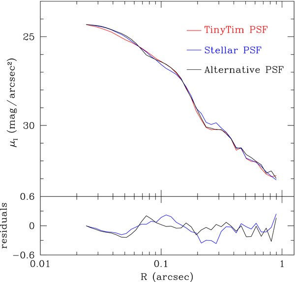
Figure 1. Comparison of the radial profiles of three different PSF models. The red line is the PSF model generated by Tiny Tim for the galaxy SDSSJ084234.50+031930.6. The blue line is for the bright star in the image of this galaxy. The black line is for a PSF model in the WFPC2 PSF library. They are all normalized to an arbitrary surface brightness at 002.
Download figure:
Standard image High-resolution image3.2. Determining the Sky Level
The sizes of the images are 800 × 800 pixels and most galaxies extend to a radius of ∼100–200 pixels or ∼5''–10''. To determine the sky level we start with a circular region with a radius of 350 pixels located at the center of the galaxies. In this way, on the one hand, we can exclude the noise near the edges of the images, while on the other hand we can make use of a large number of pixels. Then we use the command ellipse within IRAF, which follows the methods described in Jedrzejewski (1987), to derive the one-dimensional radial profile of the galaxy. Obvious contaminating features such as bright stars and small galaxies are masked. Typically, the radial profile will converge to an almost constant value at the outer radii. We take the average value of the two to four outermost radial bins in the profile to be the sky value, which will be used in our fitting. We also measure the fluctuations in values at each radius in these outermost bins to estimate the random error, which is typically ∼1% of the sky value. When there are contaminants nearby, the standard deviation can reach 5% of the sky value.
In cases where the primary galaxy is compact and there are multiple stars or galaxies in the field, we use a smaller region for the sky determination. In cases where the galaxy is very extended (e.g., SDSS J110501.97+594103.6), we use observations in the three WF chips to determine the sky value. Finally, there are some galaxies with inclined disks that almost fill part of the image while leaving other parts almost empty. In these cases we put rectangular regions along the galaxy minor axis and use these regions to measure the sky counts and standard deviation.
As the measured galaxy sizes are very sensitive to the adopted sky value, we check the sky values in a few ways. For the 17 most extended galaxies, we create a radial profile extending beyond the PC chip, and calculate the average sky value where the profile becomes constant. In addition, we calculate the average counts in a few randomly chosen blank regions. Results from these different methods agree with the adopted values within 2σ, which means the sky values and uncertainties we adopt are well defined. There is another way to measure the sky value using the mode, or most common pixel value. This determination should be less affected by contamination. The sky values determined from the mode agree with our adopted value within one standard deviation. Another consistency check is described in the Appendix.
3.3. Parametric Fitting with GALFIT
Following Greene et al. (2008), we use the GALFIT routine to perform full two-dimensional profile decompositions (e.g., Peng et al. 2002, 2010) with the following goals. First, we want to determine what fraction of the galaxies contain various components, such as bulges, disks, and bars. Second, we wish to measure the bulge properties (luminosity and size) to study the bulge scaling relations (e.g., the fundamental plane) for these galaxies. Third, we will quantify the morphology of the galaxies based primarily on the bulge-to-total (B/T) light ratio (e.g., Simien & de Vaucouleurs 1986). Two-dimensional fitting has the benefit that different components can be modeled with different position angles (P.A.s). PSF convolution is included in a straightforward way. Also, complex components such as nuclear disks and bars can be included. GALFIT models the galaxy components as axisymmetric ellipsoids. Lopsided components can also be modeled with the most recent version, GALFIT 3.0 (Peng et al. 2010), which we use here.7
In general, we proceed as follows. First, we look at the image and the one-dimensional radial profile to determine what components to include in our model. Sometimes there is an obvious bar or disk in the galaxy, which is included in the fitting. Most of the time, there are no distinguishing structures and we perform an initial fit with a central PSF for the AGN and a generalized Sérsic model:
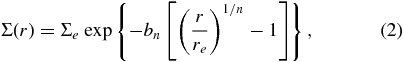
where re is the effective (half-light) radius, Σe is the surface brightness at re, n is the Sérsic index, and bn is chosen so that the region within re contains half of the light in the profile integrated to infinity.
For n = 1, the Sérsic model is reduced to an exponential profile. Exponential profiles are usually used to describe disks. The exponential profile is written in another form:
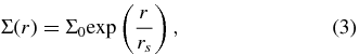
where Σ0 is the central surface brightness and rs is the radius at which the surface brightness drops to 1/e of the central surface brightness. In this paper, the disk size is reported with rs while for other components we report re. For n = 1, there is a simple relation re = 1.678rs.
For n = 4, the Sérsic profile is equivalent to a de Vaucouleurs (1948) profile, which is often used to describe the light profile of elliptical galaxies. In GALFIT, if we let the Sérsic index n float freely, GALFIT will sometimes adopt an unacceptably large n to reduce the χ2. As shown in Blanton & Moustakas (2009), most nearby galaxies have a Sérsic index smaller than 5. During our fitting, we fix n = 1, 2, 3, 4, respectively, for the bulge component and see which gives the best fit. Other groups (e.g., Benson et al. 2007; Simmons & Urry 2008) adopt a similar strategy of fixing the Sérsic index to discrete values. If different n values give almost the same parameters and the same reduced χ2, then we cannot distinguish between the different Sérsic models. For the bar component, we model the intensity distribution with n = 0.5 (e.g., Freeman 1966; Greene et al. 2008), which is a Gaussian profile.
In order to determine whether a galaxy has bar structure, we visually check the images one by one, since a weak bar may exist even when the outer parts of the galaxy are well fit by a single n = 1 component. For the ambiguous cases when we cannot distinguish between a bar or edge-on disk visually, we check the ellipticity profile and the P.A. profile as described in Menéndez-Delmestre et al. (2007). We use the ellipse command in IRAF to plot ellipticity and P.A. at each radius. For the galaxies with a round bulge at the center, we should see a monotonic increase in ellipticity and a constant P.A. across the bar. Because the bar and the disk usually have different P.A.s, we should also see the ellipticity drop abruptly while the P.A. changes sharply at the end of bar. If we see those signatures simultaneously, we conclude that there is a bar. If either signature is missing and we do not see a bar clearly by eye, we do not classify the galaxy as barred. In Figure 2, we show two examples of this procedure. For galaxy 0823 + 0606, we see both a sharp drop of the ellipticity profile and an almost constant P.A. profile indicative of a bar. For galaxy 0833 + 0620, although there is a change in the ellipticity profile at ∼50 pixels, the P.A. changes with radius and we also do not see a bar-like structure in the image. This galaxy has no large-scale bar.
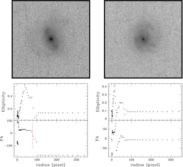
Figure 2. Example ellipticity and P.A. profiles that are used to determine whether or not a given galaxy contains a bar. The left panels are for galaxy 0823+0606 while the right panels are for galaxy 0833+0620. The top two images are 300 × 300 pixels in size. In the bottom left panel, the sharp drop in ellipticity around 60 pixels (red dashed line) and the constant P.A. confirm the bar we see in the image. In the bottom right panel, although we see changing ellipticity and P.A. around 50 pixels, we do not see any bar-like structure in the image. The change in ellipticity is likely influenced by the spiral arms so that the P.A. is not constant.
Download figure:
Standard image High-resolution imageAfter we find the best fit with the AGN component and one Sérsic model, we compare the radial profile of the model and the image and decide whether we need to add a new component. We continue in this way until the model fits the image. Our criteria are that there be no large features in the one-dimensional residuals and that the reduced χ2 has a minimum of ∼1.
Note that we are not fitting the spiral arms or knots of star formation and other nonaxisymmetric features, which are apparent in some of the residual images. However, we do fit additional compact components in the central region if necessary, which means any component with an effective radius smaller than the re of bulge. In some cases, without this nuclear component there is also extra light in the residuals regardless of the value of n. A similar nuclear component with size ∼100 pc is also found in the nearby low-mass AGN host POX 52 (e.g., Barth et al. 2004; Thornton et al. 2008). This is different from nuclear star clusters in late-type galaxies, which have typical radii ∼2–5 pc (e.g., Böker et al. 2004). As the median redshift of our sample is 0.085, a nuclear star cluster will fall within a single WFPC2 pixel. The bright nuclear point source only makes the situation worse. Therefore, unfortunately, we do not have sufficient angular resolution to search for nuclear star clusters in our sample.
4. UNCERTAINTIES AND UPPER LIMITS
In our GALFIT modeling there are two factors that dominate the fitting uncertainties: the PSF model and the sky level. Uncertainty in the magnitude of the AGN component is mainly due to uncertainties in the PSF model, while the sky value gives the biggest uncertainties in the sizes of extended components. When running GALFIT, we use the PSF model generated by Tiny Tim for each galaxy. To estimate the uncertainty due to the PSF model, we fit all the galaxies again with the other two PSF models as shown in Figure 1. The alternative PSF models have a similar radial profile to the Tiny Tim PSF with some differences in the wings. When we refit the galaxies with alternate PSF models, all fitting parameters are fixed except the PSF model and the component magnitudes and sizes. Then we calculate the differences between the magnitudes and sizes of different components between the new fits and the original fits, which are caused by different PSF models.
To estimate uncertainties due to the sky level, we change the sky value and fix all other parameters to their best-fit values (keeping the same PSF model). We test three different sky values. First, we allow the sky to be a free parameter in GALFIT. Then we increase and decrease the sky level by one standard deviation (see Section 3.2 for details of the sky determination). Then we calculate the differences in the magnitudes and sizes of different components between the new fits and the original fits. The largest difference is taken to be the measurement uncertainty, which is given in Table 2 and the original fitting results are reported as our best fits.
Table 2. Components of the Galaxies
| Nonparametric | Parametric | ||||||||||||
|---|---|---|---|---|---|---|---|---|---|---|---|---|---|
| Disk | Bulge | ||||||||||||
| AGN | Galaxy | AGN | rs | n | re | Bulge/ | Others | ||||||
| No. | mI | mI | mI | (kpc) | mI | (kpc) | mI | Galaxy | |||||
| (1) | (2) | (3) | (4) | (5) | (6) | (7) | (8) | (9) | (10) | (11) | |||
| 0022−0058 | 18.7 | 18.3 | 19.3 ± 2.9 | 1.28 ± 0.19 | 18.43 ± 0.16 | 2 | 0.55 ± 0.43 | 19.40 ± 0.37 | 0.29 | ||||
| 0024−1038 | 18.7 | 17.1 | 20.6 ± 1.8 | 1.22 ± 0.85 | 17.10 ± 0.01 | 2 | 0.14 ± 0.007 | 18.93 ± 0.10 | 0.16 | ||||
| 0117−1001 | 19.2 | 18.7 | 19.3 ± 0.4 | 10.76 | >17.80 | 2,3,4 | 2.36 ± 0.10 | 18.40 ± 0.03 | 1.00 | ||||
| 0120−0849 | 19.8 | 18.8 | >21.2 | 2.44 ± 1.90 | 18.95 ± 0.07 | 2,3,4 | 0.31 ± 0.06 | 19.28 ± 0.02 | 0.42 | ||||
| 0158−0052 | 19.5 | 17.7 | 20.6 ± 0.5 | 7.21 | >17.01 | 3 | 1.58 ± 0.07 | 17.42 ± 0.03 | 1.00 | ||||
| 0228−0901 | 19.8 | 17.0 | 20.7 ± 1.3 | 2.15 ± 0.55 | 17.01 ± 0.02 | 2,3,4 | 0.21 ± 0.08 | 20.35 ± 0.29 | 0.04 | ||||
| 0233−0748 | 18.8 | 14.8 | 20.8 ± 0.4 | 1.69 ± 0.29 | 15.56 ± 0.10 | 2 | 0.61 ± 0.05 | 15.92 ± 0.09 | 0.42 | ||||
| 0240+0103 | 21.2 | 19.4 | 20.0 ± 1.1 | 3.39 | >19.20 | 2,3 | 0.74 ± 0.33 | 19.80 ± 0.29 | 1.00 | ||||
| 0304+0028 | 16.9 | 14.9 | 17.9 ± 0.3 | 5.05 ± 1.20 | 14.74 ± 0.23 | 3 | 0.19 ± 0.11 | 16.68 ± 0.06 | 0.12 | Bar | |||
Notes. Column 1: abridged SDSS name for this galaxy. Column 2: nonparametric magnitude (mag) for the AGN component. Column 3: nonparametric total magnitude (mag) for the host galaxy. Column 4: parametric magnitude (mag) for the AGN component. Column 5: scale length rs (kpc) of the exponential extended disk. Column 6: parametric magnitude (mag) of the extended disk in the I band. Column 7: Sérsic index for the bulge component in the best GALFIT model. Multiple values means that GALFIT cannot distinguish between them. Column 8: effective radius of the bulge component in the Sérsic model. Column 9: parametric magnitude (mag) of the bulge in the I band. Column 10: bulge-to-total host galaxy luminosity ratio. Column 11: other components in best GALFIT model besides the extended disk and bulge. Details are given in Table 3.
Only a portion of this table is shown here to demonstrate its form and content. A machine-readable version of the full table is available.
Download table as: DataTypeset image
For galaxies with no detected bulge or conversely no extended disk component, we estimate an upper limit on these components. The effective size of the undetected component is determined according to the relationship between bulge and disk size given in MacArthur et al. (2003), which is 〈re/rs〉 = 0.22 ± 0.09. Here, re is the effective size of the bulge component while rs is the size of the extended disk. Take, for example, a galaxy with a detected bulge component but no detected extended disk. In GALFIT, we add an exponential disk component with the size fixed according to the above relation and the measured bulge size. The axis ratio of the disk component is fixed to unity as we want to estimate the upper limit for a face-on disk. The parameters of all the other components in GALFIT are kept fixed. In each case, we fix the magnitude of the disk component to be a certain value and we let GALFIT calculate the new χ2. We increase the magnitude of the undetected component until χ2=1 (or until χ2 increases by 10% in cases where χ2 starts out larger than 1). This magnitude is taken to be the upper limit of the undetected disk. The upper limit on an undetected bulge component is determined in a similar fashion. There are also six galaxies that do not include an AGN component for the best fits. We estimate an upper limit on the AGN in a similar fashion, by increasing the PSF magnitude until the final χ2 = 1. This PSF magnitude is taken as the upper limit of an AGN component. Two of the six galaxies are labeled as "c" by Greene & Ho (2007b), which means that the broad-line masses are very uncertain. All six galaxies have very bright bulge or disk components, which makes the AGN magnitude very uncertain. The chosen value of χ2 that we use to estimate the upper limit is a bit arbitrary. Nevertheless, this procedure gives us some useful information on the magnitude of the undetected component.
In order to minimize the effect of systematic uncertainties, we have followed several general principles during the fitting. We have looked at all the images one by one to identify the bar and spiral structures. The disk component is always fitted by an exponential profile as in nearby inactive galaxies, although disk profiles do vary at large radii (e.g., Pohlen et al. 2004; Erwin et al. 2005). In this way we will not be confused by different choices of Sérsic index for the disk. Whenever we decide that there is a bar component, we also add a disk component to get a physically reasonable model. During the fitting, we guess the sizes of each component based on the one-dimensional profile and take the guess as an initial value for GALFIT so that it will converge on reasonable results. For additional checks on the photometry, see the Appendix.
5. GALAXY MORPHOLOGY
We have selected a sample of galaxies with the lowest BH masses known. Based on the SDSS imaging, the galaxies have relatively low masses as well, with magnitudes ∼1 mag below L*. Now, with detailed image decompositions in hand, we are in a position to address the morphology of the host galaxies. Galaxy structure (e.g., Sérsic index, the presence of bars or nuclear spirals) will help us determine whether each bulge is a classical or pseudobulge (Kormendy & Kennicutt 2004; Fisher & Drory 2010). We quantify the bar fraction, since bars have been suggested as a feeding mechanism for low-level AGN activity (e.g., Shlosman et al. 1990). We also count the number of galaxies with interacting companions.
5.1. Statistical Results
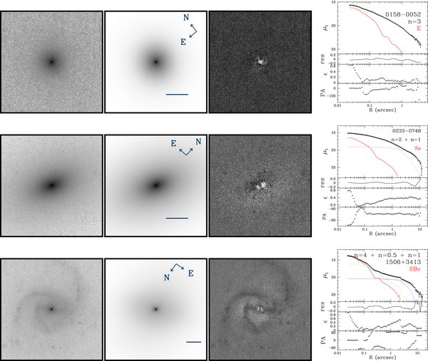
With our image decompositions we only fit the main components of the galaxies, including bulges, extended disks, bars, and nuclear structures. Spiral and irregular structures, such as nuclear spirals or rings, are not fitted and those structures can be seen in the residual images. In Figure 3, we show some example HST images, including the model image, the residual image, and a radial profile.8 The models generally match the data well.
Download figure:
Standard image High-resolution image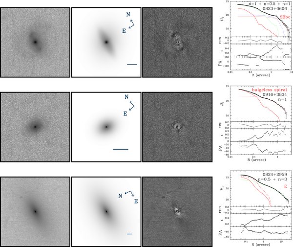
Figure 3.
Examples of HST images and GALFIT decompositions. From left to right, we show the HST image, the model image, the residual image, and the one-dimensional profile. We plot the radial profile of the AGN (solid red line), the bulge (dashed green line), the extended disk (dashed red line), and the bar (dashed blue line). The Sérsic index of each component is labeled in order of increasing size (re) of that component. These six examples include galaxies with most combinations of different components. Note that the stretch of the residual images is different from the original images. The counts in the residual images are only ∼±2% of those in the original images. Similar figures for all objects are included in the online journal. (A color version and the complete figure set (147 images) are available in the online journal.)
Download figure:
Standard image High-resolution imageIn our sample of 147 galaxies, 136 (93%) have extended disks. Of the disk galaxies, 53 of them (39%) have bars. The bar properties are shown in Table 3. Of the galaxies with disks, only seven are consistent with having no bulge component at all. The remaining 11 diskless systems are smooth and featureless galaxies. Based on their position in the fundamental plane (Section 6.1), we will argue that these galaxies are spheroidal, rather than elliptical, galaxies. Half of the diskless galaxies have a Sérsic index n > 2, which is larger than the average Sérsic index of the whole sample but similar to POX 52 (e.g., Thornton et al. 2008). However, in general their luminosities and sizes are larger than POX 52. The average absolute bulge luminosity and bulge size of these 11 galaxies are both larger than the average values of the whole sample. As listed in Table 4, four of those galaxies have an additional compact component with a size that is smaller than the effective radius of the bulge. Finally, there are seven galaxies consistent with having no bulge component at all. Details are given below.
Table 3. Galaxies with Bar Structure
| Name | Bar | |
|---|---|---|
| mI | re | |
| (mag) | (kpc) | |
| (1) | (2) | (3) |
| 0304+0028 | 16.22 ± 0.22 | 2.64 ± 0.12 |
| 0731+3926 | 17.93 ± 0.04 | 4.62 ± 0.04 |
| 0748+4540 | 19.13 ± 0.05 | 4.88 ± 0.05 |
| 0750+3157 | 17.92 ± 0.04 | 4.56 ± 0.05 |
| 0806+2419 | 18.08 ± 0.32 | 0.48 ± 0.02 |
| 0815+2506 | 19.73 ± 0.09 | 1.04 ± 0.04 |
| 0818+4729 | 18.72 ± 0.02 | 0.85 ± 0.01 |
| 0823+0651 | 19.01 ± 0.12 | 4.73 ± 0.19 |
| 0823+0606 | 18.45 ± 0.16 | 3.70 ± 0.06 |
| 0824+0725 | 16.90 ± 0.03 | 6.04 ± 0.67 |
| 0830+0847 | 19.47 ± 0.07 | 2.25 ± 0.06 |
| 0843+3610 | 16.70 ± 0.16 | 10.63 ± 0.27 |
| 0847+3604 | 18.56 ± 0.12 | 2.56 ± 0.03 |
| 0854+0808 | 18.38 ± 0.10 | 8.05 ± 0.55 |
| 0900+4327 | 17.22 ± 0.05 | 4.16 ± 0.37 |
| 0903+4639 | 19.18 ± 0.07 | 1.96 ± 0.05 |
| 0910+0408 | 18.96 ± 0.14 | 4.23 ± 0.14 |
| 0925+0502 | 19.10 ± 0.11 | 2.72 ± 0.09 |
| 0927+0843 | 18.21 ± 0.33 | 2.67 ± 0.15 |
| 0933+5347 | 18.22 ± 0.14 | 4.31 ± 0.16 |
| 0940+0324 | 17.62 ± 0.05 | 1.97 ± 0.02 |
| 0942+4800 | 19.69 ± 0.04 | 2.07 ± 0.06 |
| 0942+0838 | 18.17 ± 0.19 | 7.83 ± 0.25 |
| 0953+3650 | 19.90 ± 0.17 | 0.47 ± 0.06 |
| 0953+5626 | 18.39 ± 0.02 | 1.74 ± 0.01 |
| 1022+3837 | 19.76 ± 0.07 | 3.50 ± 0.07 |
| 1029+4314 | 17.80 ± 0.05 | 4.13 ± 0.08 |
| 1043+5121 | 16.95 ± 0.03 | 5.56 ± 0.07 |
| 1048+4133 | 18.32 ± 0.07 | 3.71 ± 0.04 |
| 1051+6059 | 17.68 ± 0.09 | 6.00 ± 0.13 |
| 1057+4825 | 18.06 ± 0.03 | 1.78 ± 0.01 |
| 1102+4638 | 18.14 ± 0.14 | 0.53 ± 0.02 |
| 1105+5941 | 15.52 ± 0.02 | 1.74 ± 0.01 |
| 1123+4331 | 17.87 ± 0.07 | 3.49 ± 0.12 |
| 1126+5134 | 16.56 ± 0.07 | 1.96 ± 0.03 |
| 1151+5613 | 17.39 ± 0.12 | 3.59 ± 0.10 |
| 1153+4612 | 16.25 ± 0.07 | 3.56 ± 0.04 |
| 1258+5225 | 19.94 ± 1.31 | 5.37 ± 0.37 |
| 1313+0519 | 17.73 ± 0.43 | 2.89 ± 1.23 |
| 1325+5429 | 19.12 ± 0.16 | 3.77 ± 0.27 |
| 1342+4827 | 19.58 ± 0.06 | 1.39 ± 0.08 |
| 1416+5528 | 16.90 ± 0.30 | 6.65 ± 0.18 |
| 1435+3413 | 18.71 ± 0.04 | 1.22 ± 0.01 |
| 1437+5458 | 18.22 ± 0.02 | 0.77 ± 0.04 |
| 1506+3413 | 17.23 ± 0.04 | 5.30 ± 0.19 |
| 1546+4751 | 18.97 ± 0.04 | 2.90 ± 0.01 |
| 1617−0019 | 19.83 ± 0.05 | 1.00 ± 0.02 |
| 1621+3436 | 18.55 ± 0.07 | 3.58 ± 0.08 |
| 1708+6015 | 18.22 ± 0.16 | 9.34 ± 0.09 |
| 2137−0838 | 19.38 ± 0.10 | 3.32 ± 0.30 |
| 2211−0105 | 19.18 ± 0.05 | 5.45 ± 0.23 |
| 2238+1433 | 18.80 ± 0.06 | 4.80 ± 0.03 |
| 2358+0020 | 19.56 ± 0.07 | 4.56 ± 0.06 |
Notes. Column 1: abridged SDSS name. Column 2: the I-band magnitude of the bar component. Column 3: effective size of the bar component.
Download table as: ASCIITypeset image
Table 4. Galaxies with Compact Nuclear Components
| Name | Compact Nuclear Component | |
|---|---|---|
| mI | re | |
| (mag) | (kpc) | |
| (1) | (2) | (3) |
| 0824+2959 | 16.63 ± 0.01 | 0.093 ± 0.001 |
| 1153+5256 | 18.62 ± 0.22 | 0.91 ± 0.22 |
| 1223+5814 | 17.54 ± 0.02 | 0.148 ± 0.004 |
| 1656+3714 | 19.63 ± 0.40 | 0.17 ± 0.06 |
Notes. Column 1: abridged SDSS name. Column 2: the I-band magnitude of the nuclear component. Column 3: effective size of the nuclear component.
Download table as: ASCIITypeset image
5.2. Interacting Galaxies
Mergers are believed to be an efficient way to trigger AGN activity and feed gas to the central supermassive BH (e.g., Hopkins & Quataert 2010; Mayer et al. 2010). Mergers are also thought to trigger star formation in galaxies (e.g., Barton et al. 2000, 2007; Blanton & Moustakas 2009). Observations have found examples of mergers in AGNs with more massive BHs. (e.g., Liu et al. 2010). For our sample of low-mass BHs, we can check whether or not mergers are a common and important phenomenon.
In our sample, 13 of the galaxies (9%) are detected with close companions that are likely physically interacting. Some of them show obvious long tails, which are clear signatures of tidal interaction. In Figure 4, we show six example interacting galaxies. Although the fraction of interacting galaxies in our sample is only ∼9%, it is already larger than the 1%–2% reported for luminous galaxies (e.g., Blanton & Moustakas 2009). However, we caution that we identify the companions only visually based on our HST images. We do not use well-defined criteria, nor do we have a well-defined control sample to compare it with (e.g., Woods & Geller 2007; Darg et al. 2010) as this is not our main focus.
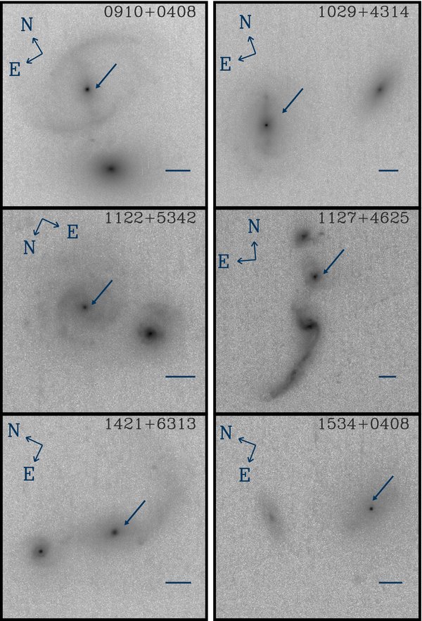
Figure 4. Interacting galaxies. Here we show six examples of close interacting galaxy pairs. Some of them have obvious tidal tails (1127+4625 and 1421+6313). There are 13 such galaxies in our total sample of 147 galaxies. The arrow indicates the program galaxy in each case. The scale bars are 2''.
Download figure:
Standard image High-resolution image5.3. Bulge-to-Total Ratio
The ratio between the bulge and total light (B/T; the AGN is excluded) varies from 0 (no bulge detected) to 1 (for spheroidal galaxies). The mean value is 〈B/T〉 = 0.28 with a median of 0.18. In most cases B/T is either less than 0.5 or greater than 0.9, with only 15 galaxies in between. If we restrict our sample to those galaxies with a detected disk component, then the mean becomes 〈B/T〉 = 0.23 with a median value of 0.16. In this case, the ratio is always <0.85.
Based on B/T, we can assign a Hubble type to each galaxy following the Third Reference Catalogue (RC3; Simien & de Vaucouleurs 1986; de Vaucouleurs et al. 1991). For the 129 galaxies with a detected disk and bulge component, we find: 2% are Hubble-type E; 15% are Hubble-type S0; 18% are Hubble-type Sa; 28% are Hubble-type Sb; 30% are Hubble-type Sc; and the remaining 7% are Hubble-type Sd. A histogram for the Hubble-type distribution is given in the bottom panel of Figure 5, which shows that our sample peaks at Hubble-type Sbc to Scd.
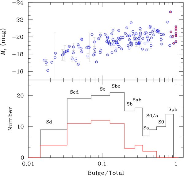
Figure 5. Top: relation between bulge-to-total ratio and bulge magnitude. Galaxies without a detected extended disk are labeled with red triangles (note that those with a bulge-to-total ratio less than one have a nuclear component). Bottom: histogram of the bulge-to-total ratio, from which we can see the distribution of galaxies in terms of Hubble type. The red line is the histogram for galaxies with bars. Note that the galaxies labeled with "Sph" have Hubble-type "E." But they are not elliptical galaxies. Instead, they are similar to spheroidal galaxies according to their positions in the fundamental plane.
Download figure:
Standard image High-resolution imageIn the top panel of Figure 5, we also show the relationship between the bulge magnitude and B/T. This plot clearly shows that B/T is larger when the bulge luminosity is larger. In other words, when the bulge becomes more luminous, the disk component becomes relatively faint. It is clear that some of the bulge magnitudes are very uncertain, particularly at low values of B/T. The uncertainty in the bulge magnitude is dominated by uncertainties in the PSF model, but the sky level also plays a role.
There are 27 galaxies (18% of the total sample) with B/T <5%. As the extension of these very faint galaxies, there are even some galaxies with no detected bulge component, which are described below.
5.4. Bulgeless Galaxies
As discussed in the Introduction, we are interested in how many bulgeless galaxies contain AGNs. In our sample, we find seven galaxies (5% of the sample) that are best fitted by pure disks. They are 0916+3834, 0942+4800, 0953+3650, 1102+4638, 1116+4236, 1437+5458, and 1534+0408. These galaxies are either fitted by a pure exponential disk (three) or a bar plus an exponential disk (four). The bulge magnitude limits range from <20.6 to <18.4 mag. However, because there is a bright AGN component at the center and four of them are at redshift z ≈ 0.2, a small bulge could escape detection in the HST images. Deeper and higher-resolution observations are needed to confirm their bulgeless nature. Such a small number of bulgeless galaxies with AGN activity even in such a large sample suggests that these systems are truly rare, although the SDSS selection does introduce a bias against faint galaxies and AGNs (Greene & Ho 2007a).
5.5. Bars and Nuclear Structures
In our sample, there are 53 galaxies with detected bars and 4 with compact nuclear components (i.e., components smaller than the bulge effective radius that require an additional Sérsic profile). Looking only at galaxies with extended disks, the bar fraction is 39%. Excluding the disk galaxies with an inclination angle larger than 60°, where it is difficult to detect a bar (e.g., Hao et al. 2009), the bar fraction drops to 37%. It is interesting to compare our sample with narrow-line Seyfert 1 (NLS1) galaxies. Like our galaxies, NLS1s are thought to have BHs with relatively modest BH masses (⩽107 M☉) and high Eddington ratios (e.g., Pounds et al. 1995; Crenshaw et al. 2003). Crenshaw et al. (2003) find that >60% of the NLS1s in their sample have a bar. The bar fraction in our sample is much smaller than that of Crenshaw et al. (2003). Actually, the bar fraction here is also smaller than that of luminous AGNs and star-forming galaxies. Based on the classification and structure information for ∼2000 galaxies from the SDSS, Hao et al. (2009) claim that the AGN optical bar fraction is 47% and that the optical bar fraction in star-forming galaxies is 50%. In inactive galaxies, the bar fraction is only 29%, which is close to that in our sample.
A relation between bar fraction and B/T is also claimed. People find that the bar fraction increases with decreasing B/T, meaning that the bar fraction is larger in disk-dominated galaxies (e.g., Marinova et al. 2009). This conclusion is also confirmed in our sample. We divide our sample into three equal bins in B/T: 0–0.33, 0.33–0.66, and 0.66–1. The bar fraction (with highly inclined "bars" excluded) in the three bins is 45%, 11%, and 0%, respectively. Histograms of the barred galaxy fractions for each Hubble type (Figure 5) shows that the bar fraction is largest in Sbc–Scd galaxies and is very small for early-type galaxies.
Some theoretical models have proposed that bar driving can be an efficient mechanism to funnel gas down to small scales where it can be accreted by the BH (e.g., Shlosman et al. 1990; Hopkins & Quataert 2010). However, observations do not find a definite connection between bars and AGN activity. For example, some groups (e.g., Ho et al. 1997; Mulchaey & Regan 1997) do not find an excess of bars in Seyfert galaxies, while other groups (e.g., Knapen et al. 2000; Laurikainen et al. 2004) claim a higher fraction of bars in Seyfert galaxies. We have also compared the AGN magnitudes for the galaxies with and without bars. The galaxies with bars do not show significantly larger AGN luminosities. We see no evidence that bars are the dominant feeding mechanism for the AGNs in our sample. Instead, the bar fraction is roughly consistent with what we expect from inactive galaxies.
6. BULGE MORPHOLOGY
We now turn to the galaxy centers, and we consider three types of centrally concentrated components: classical bulges, pseudobulges, and spheroidals. For the galaxies without disks, we are trying to distinguish between a small elliptical galaxy and a luminous spheroidal. We follow the definition of spheroidal galaxies from Kormendy et al. (2009). Spheroidals are physically small, dynamically hot stellar systems and thus are often called "dwarf elliptical galaxies." While superficially they resemble elliptical galaxies, they are much less dense at a given size or luminosity than low-mass ellipticals. Spheroidal galaxies and elliptical galaxies are located along nearly perpendicular tracks in the fundamental plane projections, presumably reflecting differences in formation history (Kormendy et al. 2009). In terms of structure, spheroidal galaxies are closer to disk, rather than elliptical, galaxies (e.g., Kormendy 1985). They are thought to be defunct spiral galaxies that lost their gas through interactions with a more massive companion. We should note that the interpretation we adopt here is not universally accepted in the literature (e.g., Gavazzi et al. 2005; Ferrarese et al. 2006; Côté et al. 2007), but we believe it is well justified by the observations (Kormendy et al. 2009).
Turning now to the disk galaxies, it is widely accepted that there are actually two kinds of bulges, which are formed in two different ways (see the review in Kormendy & Kennicutt 2004). Classical bulges are thought to form in mergers. Such bulges are similar to scaled-down elliptical galaxies in terms of their stellar populations and structural properties.
The other type of bulge is a pseudobulge. Pseudobulges are believed to be formed by secular processes, including the slow rearrangement of material by bars, oval disks, and spiral structure. Pseudobulges typically share several distinguishing properties (e.g., Kormendy & Kennicutt 2004; Gadotti 2009; Fisher & Drory 2010). First, they usually have flatter shapes and have Sérsic indices n < 2. They also often have bars, spiral structures, or rings. Second, they have a high degree of rotational support, so that the ratio between the rotation velocity and velocity dispersion is high (e.g., Kormendy & Illingworth 1983). As a corollary, they tend to have smaller velocity dispersion σ* at fixed luminosity than elliptical galaxies in the Faber & Jackson (1976) relation. Third, they have small B/T (e.g., Kormendy & Kennicutt 2004). Fourth, they are located at different positions in the 〈μe〉–re plane, where 〈μe〉 is the mean surface brightness within the effective radius re. In Gadotti (2009), the following relation is used to identify pseudobulges:

where 〈μe〉 is measured in the SDSS i band with units of mag arcsec−2. Finally, pseudobulges usually have young stellar populations and/or recent star formation. Here, we use the B/T, Sérsic index, and the presence of bars or rings to classify the bulges in our sample. We warn the reader that there is not yet a clean, well-defined, and widely accepted mathematical prescription for defining pseudobulges, especially with our limited data. By combining these different criteria, we argue that most of the bulges are likely to be pseudobulges.
Recall that our derived Sérsic indices are uncertain. However, in 76% of the galaxies, we can reliably distinguish Sérsic indices larger or smaller than 2. In our sample, 33 galaxies are best fitted with n > 2. Excluding the 7 galaxies without a bulge component, 79 galaxies (70% of the galaxies with reliable Sérsic index) have n < 2 for the bulge. Of the galaxies with a bulge component, 92% have an extended disk and ∼40% have a bar (Sections 5.1 and 5.5). There are also ring-like structures in ∼17% of our sample. As shown in Figure 5, 49% of galaxies have B/T <20% and 74% have B/T <40%. The remaining 14% of galaxies have B/T <5%. Finally, if we apply the empirical relation from Equation (4) (Gadotti 2009) to our sample, all of our galaxies with a bulge component satisfy this relation. Thus, the majority of galaxies in our sample have properties consistent with those of pseudobulges.
Now we are ready to examine where the galaxies lie in the fundamental plane (e.g., Kormendy & Kennicutt 2004). As the above evidence shows, most of our galaxies are likely to be pseudobulges. We therefore expect them to scale differently in the fundamental plane than in elliptical galaxies (Kormendy 1980; Carollo 1999; Kormendy & Kennicutt 2004; Fisher & Drory 2010). Specifically, we expect them to look more like disks. In addition to the photometric projections shown here, we also have stellar velocity dispersion measurements and present the Faber & Jackson (1976) relation in Section 6.2.
6.1. The Fundamental Plane
In Figure 6, we show three different projections of the fundamental plane. The open blue circles are our sample. All the others are comparison samples taken in the V band from Kormendy et al. (2009), Ferrarese et al. (2006), and Gavazzi et al. (2005). We choose the Virgo galaxies as a comparison here because they have very deep and uniform photometry and analysis. They constitute a clean representative sample of local red galaxies. The sample is not complete, but nicely demarcates the region occupied by elliptical and spheroidal galaxies in the fundamental plane.
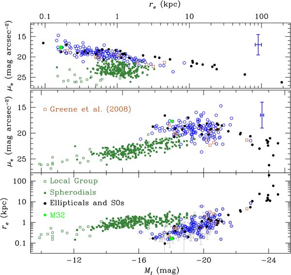
Figure 6. Fundamental plane projections of our sample, in blue open circles. We show the relations between the absolute magnitude of the bulge MI, the effective radius of the bulge re, and the surface brightness at re, μe. Bulge upper limits are not shown. For comparison, we show elliptical and S0 galaxies (filled black circles) and M32 (large green circle) from Kormendy et al. (2009), Virgo spheroidal galaxies (green filled squares) from Kormendy et al. (2009), Ferrarese et al. (2006), and Gavazzi et al. (2005), and Local Group dwarf spheroidal galaxies (open squares) from Mateo (1998) and McConnachie & Irwin (2006). Their V-band magnitudes are shifted to the I band assuming V − I = 1.34 mag (e.g., Greene et al. 2008). For spheroidal galaxies, we use V − I = 1.09 (Fukugita et al. 1995).
Download figure:
Standard image High-resolution imageIn order to properly compare the samples, we calculate the magnitude difference between the HST filters F814W and F555W9 based on a template elliptical galaxy spectrum from the Kinney–Calzetti atlas (Kinney et al. 1996) using calcphot in IRAF. The result is V − I = 1.34 mag, which is also the value used in Greene et al. (2008). We shift the comparison elliptical and S0 galaxies from the V band to the I band with this conversion factor. Spheroidal galaxies are typically bluer than elliptical galaxies. For the spheroidal galaxies, we adopt V − I = 1.09 mag, the color of Sbc galaxies listed in Table 3 of Fukugita et al. (1995), because spheroidal galaxies are redder than Scd galaxies but bluer than Sa galaxies based on the B − I color (Gavazzi et al. 2005; Greene et al. 2008).
We fit log–linear or linear relations to the fundamental plane for our galaxies with disk components, following the same fitting method as described in Greene & Ho (2006). The fitting method is based on a Levenberg–Marquardt algorithm. The intrinsic scatter is an additional error term that is chosen such that the minimum χ2 is one. Upper limits are not included in the fits. The fitting results are shown in Table 5. In the μe − re plane (the top left panel of Figure 6), our sample galaxies have a steeper scaling than that of elliptical galaxies and classical bulges. The difference is even more significant in the μe − MI plane. The fundamental plane of these pseudobulges has a different slope and normalization than the elliptical or the spheroidal galaxies, such that the faint end is closer to faint elliptical galaxies while the bright end is closer to bright spheroidal galaxies.
Table 5. Fit Results
| Our Sample | Ellipticals and S0 | ||||||||
|---|---|---|---|---|---|---|---|---|---|
| Relation | α | β |  0 0 |
Median Value | α | β | 0 |
Median Value | |
| log (re)–μe | 4.88 ± 029 | 18.53 ± 0.09 | 0.16 | −0.26 | 2.43 ± 0.16 | 19.53 ± 0.13 | 0.67 | 0.097 | |
| MI–μe | 0.53 ± 0.12 | 18.82 ± 0.13 | 0.54 | −19.42 | −0.68 ± 0.10 | 19.93 ± 0.23 | 1.31 | −20.97 | |
| MI–re | −0.17 ± 0.02 | −0.23 ± 0.02 | 0.22 | −19.42 | −0.33 ± 0.02 | 0.24 ± 0.05 | 0.26 | −20.97 | |
| Our Sample + Gültekin et al. | Gültekin et al. | ||||||||
| Relation | α | β | 0 |
Median Value | α | β | 0 |
Median Value | |
| MI–log (σ) | −0.13 ± 0.01 | 2.00 ± 0.02 | 0.07 | −20.37 | −0.10 ± 0.01 | 2.32 ± 0.02 | 0.06 | −22.52 | |
Notes. We fit y = α × (x − x0) + β, where x (the independent variable) is listed first in Column 1 and y (the dependent variable) is listed second. x0 is the median value of x and is kept fixed. 0 is the intrinsic scatter. All the fits are done on the original data before corrections for stellar age are applied.
Download table as: ASCIITypeset image
Previous results have also found that the photometric scaling relations of pseudobulges diverge from those of classical bulges. Carollo (1999) finds that their "exponential" (or pseudo) bulges span a much wider range of effective surface brightnesses than do classical bulges and elliptical galaxies. Fisher & Drory (2010) present a similar result. They see almost no dependence of effective surface brightness on effective radius. Our findings are similar over the range of effective radius that we share. Thus, the observed scaling relations also support our assertion that our disk sample is dominated by pseudobulges.
There are 11 galaxies without extended disks. These systems are more challenging to interpret. On the one hand, they are typically 2 mag more luminous than luminous spheroidal galaxies (green squares in Figure 7). However, they are larger and have lower surface brightnesses than faint ellipticals of their luminosity. The difference is most significant in the μe − re plane (the top panel of Figure 7). Thus, as in Greene et al. (2008), we conclude that the sample is made up predominantly of spheroidal systems whose luminosities are boosted by ongoing star formation. As we will see in the next section, their scaling in the Faber–Jackson relation strengthens our conclusion here (Section 6.2).
Figure 7. Expanded view of the region containing our sample in Figure 6. All the symbols are the same as in Figure 6. We highlight galaxies without a detected extended disk (red triangles) and the 18 objects from Greene et al. (2008, brown squares).
Download figure:
Standard image High-resolution image6.1.1. Stellar Population Effects
It is important to note that our sample galaxies likely contain younger stars on average than Virgo cluster galaxies. Unfortunately we do not have direct measurements of the bulge colors. However, inactive spiral galaxies at these masses are all bluer than more massive galaxies (e.g., Roberts & Haynes 1994). This is also true for bulges (e.g., Bender et al. 1992). Furthermore, it is likely that some of the nuclear structures represent ongoing or recent star formation. One way to compensate for this difference is to estimate the mass-to-light ratio (M/L) for the bulges. We can estimate their dynamical M/L using σ* observations. The bulge virial mass can be estimated as ∼6.5 reσ2/G (e.g., Taylor et al. 2010), where G is the gravitational constant. We find an average M/L in our sample of ∼1.8 (in units of M☉/L☉). For a typical elliptical galaxy in the I band, the M/L is ∼4–6 (e.g., Cappellari et al. 2006). If we keep the stellar mass fixed but imagine that the stars evolve to the same age as those in elliptical galaxies, the luminosity would be decreased by a factor of 2.2–3.3, corresponding to an increase of 0.8–1.3 mag. Although we do not know the bulge M/L for individual galaxies, we can take the average impact of fading the stellar populations to be ∼1 mag.
Applying a shift of 1 mag to our sample, the fundamental plane would then appear as shown in Figure 8. This average accounting for stellar population effects only strengthens our conclusions. Our galaxies occupy a different region of the fundamental plane from elliptical/S0 galaxies. At the bright/large end, the galaxies clearly deviate from the fundamental plane of massive elliptical galaxies. However, at the faint/compact end, the galaxies are more consistent with the fundamental plane of small elliptical galaxies like M32 than they are with spheroidals of the same size or luminosity. In addition, the locus of the diskless galaxies moves closer to that of the spheroidal galaxies.
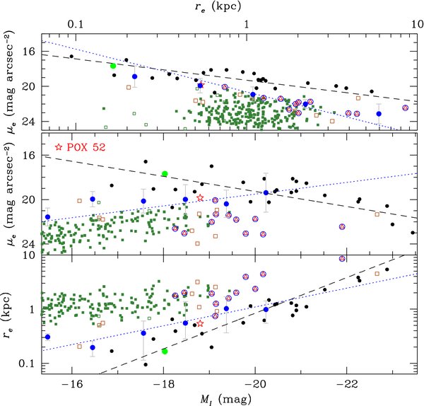
Figure 8. Same fundamental plane plot as Figure 6, except that we shift the sample by 1 mag to account crudely for differences in stellar populations between our sample, which likely contains some young stars, and the uniformly old elliptical galaxies. All other comparison samples are the same as in Figure 6. The filled blue circles are median values of re and μe in uniform bins of MI or re, respectively, for the galaxies with extended disks. The dashed black lines are best-fitting relations for elliptical galaxies and classical bulges (Table 5). The blue dotted lines are best-fitting relations for our galaxies with extended disks with the 1 mag shift applied (shifting the relations from Table 5 by 1 mag).
Download figure:
Standard image High-resolution image6.2. The Faber–Jackson Relation
We have considered photometric projections of the fundamental plane. For a subset of galaxies, we can also examine the Faber & Jackson (1976) relation between stellar velocity dispersion (σ*) and bulge luminosity. Previous results suggest that pseudobulges demonstrate considerably larger scatter in the Faber–Jackson relation, with a tendency to have a lower σ* at a given luminosity (e.g., Kormendy & Illingworth 1983; Dressler & Sandage 1983; Kormendy & Kennicutt 2004; Greene et al. 2008). We examine the situation for our sample.
We have σ* measurements for 34 galaxies in the sample. The data were taken at Keck with ESI and at Magellan with MagE. The measurements are based on direct-pixel fitting of broadened stellar templates to the galaxy spectra (Barth et al. 2005; Xiao et al. 2011). For the remaining objects, we do not have direct stellar velocity dispersion measurements. Instead, we use the widths of forbidden lines from the narrow-line region as an approximate indicator of the stellar velocity dispersion. In most AGNs, the widths of low-ionization emission lines, such as [O ii] and [S ii], are a good proxy for σ*, as shown in Nelson & Whittle (1996) and Greene & Ho (2005a), and then discussed in detail in Ho (2009). In this paper, we refer to dispersions based on [S ii] as σgas, which are used whenever we have no σ* measurement.
6.2.1. Restricted Sample
In these disk-dominated galaxies, the observed σ* of the bulge can be contaminated by rotationally dominated disk light. At Keck we employed a slit of 075 while at Magellan we used a 1'' slit (Barth et al. 2005; Xiao et al. 2011). If the bulge size is smaller than the slit size and the bulge is much fainter than the disk component, then the observed σ* will be contaminated by light from the disk. Since σ* is a luminosity-weighted measurement, the contamination will artificially increase σ* in an edge-on system, and could slightly lower it in a face-on system. Here, we evaluate whether and in what sense disk light contamination is important. We divide our sample into four bins based on bulge re: 60% of the bulges have re < 037, 22% have 037 < re < 075, 6% have 075 < re < 1'', and the rest (12%) have re > 1''. Compared with our slit sizes, we conclude that disk contamination can be significant.
As an additional test of the effect of disk contamination, we look for trends as a function of the galaxy inclination. We use our photometric fits to divide the sample with σ* measurements into three equal inclination bins containing 10 galaxies each. Extrapolating the Faber–Jackson relation of classical bulges defined by the sample from Gültekin et al. (2009) to low luminosities, we calculate a predicted velocity dispersion σpredict from the observed magnitude. We define the average difference as 〈σpredict − σ*〉. From edge-on galaxies to face-on galaxies, we find 〈σpredict − σ*〉 = 9, 20, 32 km s−1 for the three bins, respectively. The galaxies with the highest inclination are those that suffer the most contamination. On average, they also have the highest dispersions at fixed luminosity. Thus, the disk contamination tends to boost the observed stellar velocity dispersions.
To avoid the complexity caused by disk contamination, we define the subset of galaxies with stellar velocity dispersion measurements from the ESI/MagE spectra and extended bulges with re > 037 to be the clean sample. Most of the following analysis will be focused on this restricted sample.
6.2.2. Results
In Figure 9, we show the relation between I-band bulge magnitude and bulge velocity dispersion σ* in the host galaxy. The clean restricted sample is labeled with open blue circles filled with a black dot. We compare our results to the inactive early-type galaxies in Gültekin et al. (2009). We choose this sample because it is a well-studied representative sample of elliptical galaxies with very good measurements of luminosity and velocity dispersion. Our goal is simply to demarcate the region occupied by elliptical galaxies in this plane, so that we can compare with our sample distribution. The V-band magnitudes reported in Gültekin et al. are shifted to the I band assuming V − I = 1.34 mag as above. On average, our sample has smaller σ* at a fixed bulge magnitude than the early-type galaxies. The best-fit relations for Gültekin et al.'s sample alone and the results with the clean sample included are shown in Table 5. Our galaxies clearly have a different Faber–Jackson slope. One way to quantify the difference between our sample and classical bulges is to calculate the average difference between the observed value σ* and the predicted value σpredict, as defined in Section 6.2.1. For the clean sample, we find 〈σpredict − σ*〉 = 36 ± 8 km s−1, where the latter represents the error in the mean.
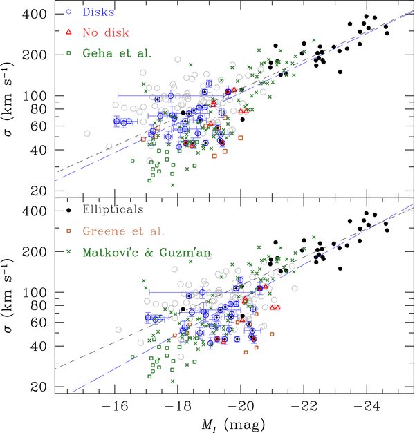
Figure 9. Bottom: Faber–Jackson relation between bulge magnitude and velocity dispersion. Open circles are our sample. Blue open circles have stellar velocity dispersions from ESI/MagE measurements (Xiao et al. 2011) while gray open circles have velocity dispersions from [S ii] line widths in SDSS spectra (Greene & Ho 2007b). We also highlight galaxies with no extended disk (red triangles) and those with low disk contamination (black solid circles; see Section 6.2.1 for details). We show the fit to the comparison sample (black solid points) from Gültekin et al. (2009) as a short-dashed line and the best fit with our sample included as the long-dashed line. The open green squares and green crosses are faint early-type galaxies from Geha et al. (2003) and Matković & Guzmán (2005), respectively. Top: the bulge magnitudes for our sample are shifted by 1 mag to account for younger stellar populations.
Download figure:
Standard image High-resolution imageWe can also quantify the difference in terms of bulge magnitude. At a fixed velocity dispersion σ*, our sample galaxies have larger luminosities on average than do early-type galaxies. We can calculate the average difference 〈Mpredict − MI〉, where Mpredict is calculated based on the observed velocity dispersion and the extrapolated Faber–Jackson relation given by Gültekin et al. (2009). For the clean sample, we get 〈Mpredict − MI〉 = 1.8 mag with the error for the mean value to be 0.4 mag.
Not only is σ* for our sample significantly smaller at a given bulge magnitude, but the scatter in the relation is also significantly larger. In order to quantify the scatter, we fit the log–linear relation log σ = α + βMI to the data. Following the fitting method used in Tremaine et al. (2002) and Greene & Ho (2006), we include an intrinsic scatter such that the reduced χ2 (Equation (1) of Greene & Ho 2006) has a best-fit value of one. The sample from Gültekin et al. (2009) alone has an intrinsic scatter of 0.064 dex. When we include our sample with σ* from ESI/MagE spectra, the intrinsic scatter is increased to 0.071 dex. As shown in Figure 9, the slope also gets steeper when our sample is included. We find effectively the same results if we include the galaxies with σgas.
By comparing the Faber–Jackson relation for our sample and early-type galaxies as shown in Figure 9, we find that our sample has systematically smaller σ* than the predicted value σpredict. This offset, like those seen in the photometric scalings above, is in the same sense as has been observed for inactive pseudobulge samples (Kormendy & Illingworth 1983). Thus, in sum, the scaling relations are consistent with the fact that >70% of our galaxies contain pseudobulges.
It is also interesting to compare the Faber–Jackson relation of our sample with inactive spheroidal galaxies. Matković & Guzmán (2005) and Cody et al. (2009) study the Faber–Jackson relation for what they refer to as "dwarf early-type" galaxies in the Coma cluster with R-band magnitudes ranging from −22.0 to −17.5 mag and −20.7 to −15.6 mag or I-band magnitudes of ∼ − 23.2 to −16.8 mag (Fukugita et al. 1995). According to their positions in the fundamental plane (e.g., Graham & Guzmán 2003), these galaxies obey our definition of spheroidal galaxies. They are found to have a relation L∝σ2, which is much flatter than the relation L∝σ4 for more luminous galaxies. As shown in Table 5, when we fit our sample (galaxies with σ* measurements) combined with that of Gültekin et al., we find L∝σ3. Specifically, the 11 diskless galaxies lie very close to the spheroidal galaxies from Matković & Guzmán (2005), and are systematically offset from the best-fit relation of elliptical galaxies. This is true even after we shift our sample to account for different stellar populations, and confirms our conclusion from Figure 7 that the diskless galaxies are actually bright spheroidal galaxies.
6.2.3. Uncertainties in the Faber–Jackson Analysis
Conclusions for the contaminated galaxies are highly uncertain, since we do not know the true σ* of these bulges. Furthermore, σgas suffers from a variety of uncertainties. However, we note that our conclusions still hold if we include the entire sample. Still, we focus on the clean sample because it is easiest to interpret.
Again, our sample likely contains younger stellar populations than the early-type galaxies, which leads to offsets in the Faber–Jackson relation. As we did for the fundamental plane relation in Section 6.1, we shift the bulge magnitudes by 1 mag (Figure 9; note that if we adopt the M/L from Table 2 of Graves & Faber (2010) for both our sample and classical bulges/elliptical galaxies, we only need to shift our sample by 0.68 mag). When we fit the relation log σ = α + βMI with the evolution correction applied, the intrinsic scatter remains high at 0.070, but the difference between the best-fit relations including and excluding our sample is no longer significant. The extent to which the offset between our sample and classical bulges is intrinsic or can be explained by stellar population differences is unclear at present. This does not apply to the spheroidal galaxies, which remain offset even with the stellar population adjustment.
7. DISCUSSION AND SUMMARY
We have looked at the host galaxies of 147 active galaxies selected to have low-mass (MBH ≲ 106 M☉) BHs. Using HST/WFPC2, we perform detailed two-dimensional bulge, disk and bar decompositions of the entire sample to study the bulge morphologies and structures of this unique sample. We find that the sample is dominated by disk galaxies (only 7% have no disk) with small bulge components.
We return to the questions we raised in the introduction. Most host galaxies of low-mass BHs have a bulge component. Only seven objects (5%) are consistent with being bulgeless galaxies. These are only candidates for bulgeless active galaxies because of the fit uncertainties, so BHs without any bulge component are apparently rare. We do have to keep in mind that we are biased by optical selection, which limits us to AGNs with high Eddington ratios in relatively massive galaxies. Multi-wavelength approaches are required to truly determine the space density of AGNs in bulgeless galaxies.
Turning to those galaxies with bulges, the only remaining question is whether they are classical or pseudobulges. Based on the low Sérsic indices, low bulge-to-total ratios, and the prevalence of bars, rings, and nuclear spirals, we argue that the disk sample is dominated by pseudobulge galaxies. Consistent with this supposition, we find that the fundamental plane of these galaxies is different from both elliptical galaxies and spheroidal galaxies, but is consistent with observations of pseudobulge fundamental plane scalings. In particular, the galaxies are larger and have lower velocity dispersions at a given luminosity than elliptical galaxies. After we account for their young stellar populations, the differences are even more significant. Our sample is also found to have a flatter Faber–Jackson relation in the L − σ plane. Of the 147 galaxies, we only find 13 galaxies with nearby companions that are candidates for ongoing mergers, which is consistent with the fact that pseudobulges evolve via secular processes. In conclusion, the host galaxies of low-mass BHs are different from classical bulges and have properties that are consistent with pseudobulges. The 11 bulges without extended disks do not scale as elliptical galaxies, either. Their fundamental plane scaling relations are systematically offset, especially in the Faber–Jackson plane. We have shown definitively that a classical bulge is not a prerequisite to host a supermassive BH.
We can also determine whether galaxies selected by their nuclear activity differ in any way from field galaxies selected at the same luminosity or mass. We have already seen that our disk galaxies have comparable bar fractions and merger fractions as inactive galaxies. We now look at the distribution of morphological types for a more complete sample of galaxies at similar luminosity. We use the morphology-dependent luminosity function from Nakamura et al. (2003). For galaxies with r*-band magnitudes Mr ≈ −18 mag, which corresponds to an I-band magnitude MI ≈ −19 mag, the relative number of elliptical/S0, Sa/Sb spiral galaxies, and Sc/Sd spiral galaxies is found to be 1.00:4.10:0.73. Our sample has relatively more late-type spiral galaxies than field galaxies selected by SDSS (Figure 5). The simplest explanation for this observed difference is that we have a bias toward spiral galaxies because they have the gas fuel needed to feed a high-luminosity AGN.
Among spirals, inactive galaxies at the luminosity of our sample are dominated by pseudobulges. Weinzirl et al. (2009) find that ∼76% of nearby high-mass spiral galaxies have low n ⩽ 2 bulges—they are pseudobulges. In a sample of 173 E-Sd galaxies, Fisher & Drory (2010) also find that over 78% of the identified bulges are pseudobulges. This implies that our AGN-selected sample has very similar bulge properties to non-AGN-selected samples.
Our results help elucidate the growth mechanisms of low-mass BHs, as they are found preferentially in pseudobulges, which are thought to be evolving secularly with a quiescent recent history (e.g., Kormendy & Kennicutt 2004). Most likely, these low-mass BHs are not fueled by major mergers, which is also consistent with the fact that only 9% of our galaxies have close companions. Rather, the secular processes that build up the bulge may well fuel the AGN as well. In fact, it is possible that these BHs were formed with a mass quite similar to their present mass (e.g., Portegies Zwart & McMillan 2002; Koushiappas et al. 2004; Begelman et al. 2006). If supermassive BHs indeed grow from low-mass BHs, some violent event (e.g., a merger) is likely required to both dramatically change the bulge properties and substantially grow the BH.
As already discussed in Greene & Ho (2007b) and Greene et al. (2010), differences in the bulge properties of low-mass BHs lead to differences in the MBH–σ* and MBH–Lbulge relations at low mass (if these relations still exist at all). The MBH–σ* relation of this sample is discussed in more detail in Xiao et al. (2011) while the MBH–Lbulge relation is discussed in a companion paper (Jiang et al. 2011). In that paper, we find that the tight scaling relations between BH mass and bulge luminosity found for massive classical bulges do not exist for the pseudobulges that we have shown are the hosts of low-mass BHs.
Y.-F.J. thanks Chien Peng for help in using GALFIT, and Minjin Kim for helpful discussions on fitting the images. We also thank the anonymous referee for valuable comments that improved the manuscript. This work was supported by the Carnegie Institution for Science and by NASA grant HST-GO-11130.01 from the Space Telescope Science Institute, which is operated by AURA, Inc., under NASA contract NAS5-26555. Research by A.J.B. is supported by NSF grant AST-0548198.
APPENDIX: TESTS OF THE PHOTOMETRY
In order to test for possible systematic biases in our fits, we estimate a nonparametric (model-independent) magnitude for each galaxy. From the counts in the image we determine the magnitude of the AGN and the galaxy as a whole. Although we cannot decompose the galaxy into different components such as bulge and disk, we derive a magnitude for the galaxy that is independent of any model assumptions.
The Tiny Tim PSF model described in Section 3.1 is used to separate the AGN component from the host galaxy in the image. The only assumption here is that the AGN component dominates the luminosity within a small aperture at the center of the galaxy and that the AGN component can be modeled by the PSF. We scale the AGN luminosity to the flux within a two-pixel radius located at the center of the galaxy. For the reasons given in Jahnke et al. (2004), we do not scale the PSF model to a single pixel at the center of the galaxy, because then we would be very sensitive to centering errors. To determine the galaxy magnitude, we first subtract the sky from each pixel in the object image. Second, we scale the PSF image so that the total counts within an aperture located at the center of the PSF image are the same as the total counts within this same aperture in the object image. The magnitude of the scaled PSF model is taken to be the nonparametric AGN magnitude. Third, we subtract the scaled PSF model from the object image. The image with the AGN model subtracted represents only the host galaxy, from which we measure a nonparametric magnitude for the host galaxy as described below.
Typically, the galaxy does not fill the whole image and there are usually other objects nearby. We thus measure the host galaxy magnitude within a region of 700 × 700 pixels in the subtracted image and mask the contaminants. There are 17 galaxies that may extend beyond the PC chip. In these cases, we create a composite image with the three WF chips and measure the sky value from these. Images from the four chips are combined with the command wmosaic in IRAF, which bins the image from the PC chip by a factor ∼2 × 2 so that the final image has a uniform pixel scale. The boundaries between different chips are also taken care of automatically by wmosaic. Images from other chips are reduced in the same manner as the PC images (see Section 2.3). While we may slightly underestimate the galaxy magnitudes, we do not include regions from the WF chips in our nonparametric magnitude estimate.
The nonparametric magnitudes of the AGN components and the host galaxies for all 147 images are given in Table 2. As pointed out in Greene et al. (2008), the host galaxies are generally much brighter than the AGNs. The median ratio between the light from the AGN and the host galaxy is only 5%. The difference between nonparametric magnitudes and the magnitudes from our fits is always <10%.
As an additional test of both our models and the sky levels in particular, we also compare the I-band total magnitudes from our models with the SDSS Petrosian r-band magnitudes as listed in Table 1 of Greene & Ho (2007b). The comparison can be seen in Figure 10. We fit a linear relation MI = α(Mr − Mr, 0) + β to the two kinds of independent magnitudes using the same fitting method described in Section 6.1 and Greene & Ho (2006). Here, we assume uncertainties in the magnitudes of 0.1 mag (the median from our fits). We find α = 1.05 ± 0.03, β = −21.30 ± 0.02, Mr, 0 = −20.31, and intrinsic scatter e0 = 0.22. This means the total magnitudes from our best fits are consistent with SDSS magnitudes at the 2σ level, and suggests that we are not introducing major systematic errors throughout our treatment of the sky.
Figure 10. Comparison between the I-band total magnitude from our best-fitting model based on HST images and r-band SDSS magnitudes.
Download figure:
Standard image High-resolution image
Footnotes
- *
Based on observations made with the NASA/ESA Hubble Space Telescope, obtained at the Space Telescope Science Institute, which is operated by the Association of Universities for Research in Astronomy, Inc., under NASA contract NAS 5-26555. These observations are associated with program GO-11130.
- 5
After improvement of the BH mass estimator, a few of the BHs have masses that are larger than this value.
- 6
- 7
More information about GALFIT can be found at GALFIT home page online: http://users.obs.carnegiescience.edu/peng/work/galfit/galfit.html.
- 8
HST images for the full list can be found in the online journal.
- 9
The difference between the magnitude through the F555W filter and the V band is smaller than 0.01 mag, as shown in Table 3 of Fukugita et al. (1995) and so we neglect the difference.