


ABSTRACT
Twist and connectivity of magnetic field lines in the flare-productive active region NOAA 10930 are investigated in terms of the vector magnetograms observed by the Solar Optical Telescope on board the Hinode satellite and the nonlinear force-free field (NLFFF) extrapolation. First, we show that the footpoints of magnetic field lines reconstructed by the NLFFF correspond well to the conjugate pair of highly sheared flare ribbons on the Ca ii images, which were observed by Hinode as an X3.4 class flare on 2006 December 13. This demonstrates that the NLFFF extrapolation may be used to analyze the magnetic field connectivity. Second, we find that the twist of magnetic field lines anchored on the flare ribbons increased as the ribbons moved away from the magnetic polarity inversion line in the early phase of the flare. This suggests that magnetic reconnection might commence from a region located below the most strongly twisted field. Third, we reveal that the magnetic flux twisted more than a half turn and gradually increased during the last one day prior to the onset of the flare, and that it quickly decreased for two hours after the flare. This is consistent with the store-and-release scenario of magnetic helicity. However, within this active region, only a small fraction of the flux was twisted by more than one full turn and the field lines that reconnected first were twisted less than one turn. These results imply that the kink mode instability could hardly occur, at least before the onset of flare. Based on our results, we discuss the trigger process of solar flares.
Export citation and abstract BibTeX RIS
1. INTRODUCTION
Solar flares are believed to be an eruptive liberation of free energy built-up in the solar coronal magnetic field. However, the triggering mechanism of solar flares is not well understood yet. The different models that have been proposed for the triggering process of flares focus on the different aspects of the stability and the equilibrium of magnetohydrodynamic (MHD) systems. Although many models emphasize magnetic twist and/or shear as an important feature for driving flares, the community has not yet reached a consensus on the issues of how strong a twist and shear within the magnetic field is necessary to trigger flares. Therefore, accurate quantification of the twist and shear of magnetic field in flaring sites is crucially important to discriminate the proposed flare models.
The solar active region (AR) NOAA 10930 is an ideal object to study of magnetic structure of flaring sites because the state-of-the-art solar physics satellite Hinode (Kosugi et al. 2007) succeeded in continuously observing the photospheric magnetic field at unprecedentedly high resolution before and after the X3.4 class flare occurred in this region on 2006 December 13. The primary objective of this paper is to quantify the magnetic twist of this region as well as to reveal the connectivity of magnetic field lines on the flaring site in terms of the vector magnetograms observed by Hinode. We also aim to clarify the critical structure of the magnetic field associated with the onset of solar flares
The twist number of the magnetic field is crucially important for the stability of magnetic flux tube. For instance, in a periodic system like a torus, more than one turn could destabilize a flux tube; this is widely known as the Kruskal–Shafranov limit (Kruskal & Kulsrud 1958). In an anchored flux tube like a coronal loop, the stronger twist is required to destabilize ideal MHD modes. Therefore, the accurate quantification of magnetic twist is necessary to judge the role of ideal MHD instabilities for the trigger of solar flares.
In this paper, we introduce a new methodology to derive the magnetic twist in terms of vector magnetograms by applying the nonlinear force-free field (NLFFF) extrapolation technique. Various authors have recently used the NLFFF extrapolation technique as a model of an AR's magnetic field (Schrijver et al. 2006; Metcalf et al. 2008; De Rosa et al. 2009; Wiegelmann 2008); however the applicability to practical data is not mature enough yet. For instance, Schrijver et al. (2008) had applied the NLFFF extrapolation to AR 10930 and found that there was a strong electric current region above the magnetic neutral line before the flare and that the strong current region disappeared after the flare. Inoue et al. (2008) also reproduced strongly sheared magnetic flux on the neutral line before the flare using their NLFFF extrapolation and found that the sheared field relaxed in part to the potential-like field after the flare.
In the following sections, we will explain the basic method of the NLFFF extrapolation (Section 2), and we will show the results of comparative analysis between flare ribbons and the three-dimensional (3D) structure of magnetic field lines (Section 3.1). Also, the spatial and temporal variation of magnetic twist in the flaring region will be analyzed in Sections 3.2 and 3.3, respectively. Finally, in Section 4, we will discuss and summarize the implication of our study for the flare trigger process.
2. NUMERICAL METHOD
There are currently several algorithms which have been developed for solving the NLFFF as a boundary-value problem (Schrijver et al. 2006; Metcalf et al. 2008; Wiegelmann 2008). For each algorithms, an optimum solution is sought numerically through an iteration process. The solution is optimized by satisfying both the force-free equation

and the photospheric magnetic field given by the vector magnetogram as the boundary condition. However, since the vector magnetogram, which corresponds to the photospheric magnetic field, does not necessarily meet the force-free condition (1), a compromising process has to be introduced to obtain the best-fit solution. This implies that care is required for evaluating the reliability of the numerically reconstructed field as the model of the coronal magnetic field, even though the iterative procedure converges. In this study, we employ the classical relaxation method, which is governed by the MHD-like equations for a pressure-less plasma,

and
to solve the force-free field. Here,  is the magnetic flux density,
  the velocity,
  the electric current density, ρ the pseudo-density, and ϕ the convenient potential. The pseudo-density is assumed to be proportional to
  in order to ease the relaxation by equalizing the Alfvén speed in space. Equation (5) was originally introduced into an algorithm for MHD calculations by Dedner et al. (2002) in order to avoid the deviation from the solenoidal condition
  . The length, magnetic field, velocity, time, and electric current density are normalized by L0 = 5.325 × 10⁹ (cm), B0 = 3957 (G), VA ≡ B0/(μ0ρ0)1/2, τA ≡ L0/VA, and J0 = B0/μ0L0, respectively. The non-dimensional viscosity ν is set as a constant (1.0 × 10⁻³), and the non-dimensional resistivity η is given by the function

where η0 = 5 × 10⁻⁵ and η1 = 1.0 × 10⁻³ in the non-dimensional unit. The second term is introduced to accelerate the relaxation to the force-free field particularly in the weak field region. The parameters ch and cp are fixed to the constant value of 0.2 and 0.1, respectively.
The vector magnetograms, which are used for the boundary condition, were provided by the observation with the spectropolarimeter (SP) of the Solar Optical Telescope (SOT) on board Hinode. In this paper, we use five magnetograms observed at 17:00 UT on 2006 December 11, 03:50 UT, 17:40UT, and 20:30 UT on 2006 December 12, and 04:30 UT on 2006 December 13. As seen in Figure 1(a), the first four images were taken before the onset of the X3.4 class flare that occurred on 2:10 UT 2006 December 13.

Figure 1. (a) Time profile of the X-ray flux measured by the GOES 12 satellite from 2006 December 11 to 14. The solar X-ray outputs in the 1–8 Å and 0.5–4.0 Å passband are plotted, respectively. Four times when magnetograms were taken are marked. (b) The hybrid magnetogram of the Hinode/SP plus the SOHO/MDI on 20:30 UT 2006 December 12. Gray scale indicates the normal component of the magnetic field (white for positive and black for negative), and the solid square indicates the area of flux integration (Equation (8)).
Download figure:
Standard image High-resolution imageThe initial guess for the iterative calculation is given by the potential field, which is derived based on a synoptic chart of the line-of-sight component of magnetic field observed by the Michelson Doppler Imager on the Solar and Heliospheric Observatory (SOHO/MDI). The global magnetic field provides the lateral and top boundary conditions of our model domain including the entire AR. The calculation starts after introducing the vector magnetogram observed by Hinode into the central part of the bottom boundary, as shown in Figure 1(b). The vector magnetograms were obtained by a Milne–Eddington inversion of Fe i lines at 630.15 nm and 630.25 nm, and the simulated annealing method was used to solve the 180° uncertainty (Leka et al. 2009). Then, we recalculate the potential field on a hybrid map (SOHO/MDI plus Hinode/SP), which has the same total magnetic flux as the original MDI map, and use it as the initial condition of the time-integral calculation for Equations (2)–(5). The numerical scheme for this calculation is given by the Runge–Kutta–Gill scheme with fourth-order accuracy for the temporal integral and a central finite difference with second-order accuracy for the spatial derivative.
The simulation domain is a rectangle box spanning (0, 0, 0) < (x, y, z) < (4.0L0, 4.4L0, 2.2L0), which corresponds to (295 2, 3246, 1623) in view angle. The domain is uniformly divided by 128 × 128 × 64 grids. The vector-field magnetogram inserted onto the bottom boundary (125 × 64 grids) has been formed by binning from the original magnetogram of 1000 × 512 pixels. We keep the longitudinal field of the SOHO/MDI map outside the SP magnetogram. The boundary condition for magnetic field is fixed for the three components of vector and the velocity is set to zero. A Neumann-type boundary condition (∂nϕ = 0) is applied to the potential ϕ over all the boundaries, where ∂n represents the derivative for the normal direction on the surface.
3. RESULTS
3.1. Comparison between Field Lines and Flare Ribbons
As mentioned in the previous section, the NLFFF extrapolation is not a fully developed technique and we should carefully evaluate its reliability. In this subsection, we show the results from comparative analysis between the connectivity of magnetic field lines derived by the NLFFF model and the observation of flare ribbons on Ca ii images taken by Hinode/SOT. Since flare ribbons are widely believed to illuminate simultaneously on the regions corresponding to the feet of reconnected magnetic field lines, we can evaluate how well the model field may capture the coronal magnetic field by inspecting the agreement between the ribbons and the feet of field lines. In addition, this analysis also helps our understanding of the connectivity of magnetic field lines in the flaring site.
Figure 2 represents the time series of Ca ii images, which is a time-differential map, observed from 02:18 UT to 02:24 UT on 2006 December 13. Overplotted are selected field lines traced from the ribbon on the negative pole. The ribbons appeared near the neutral line on 02:16 UT and grew afterward. The footpoints of field lines are marked by the letters A–G and A'–G' on the negative and the positive poles, respectively. Here, we remind the reader that the NLFFF, which was used to plot all of the field lines, was derived from the magnetogram taken at 20:30 UT on December 12, which was 6 hr prior to the onset of the flare. However, even though there is a time gap between the two different observations, we can see that the feet of the magnetic field lines correspond well to the complicated structure of the strongly sheared ribbons at all the moments shown in Figure 2. Furthermore, the line a–a' (orange in (a)) also corresponds to the brightened small arc, which has a different structure from the normal two-ribbon. All the results shown in Figure 2 indicate that the 3D structure of the magnetic field in the flaring site may be captured well by the NLFFF at least for the early phase of the flare.
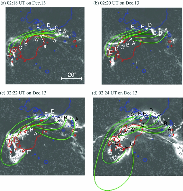
Figure 2. Magnetic field lines (green) plotted on Ca ii images (gray scale) for four different times. Field lines are traced from selected points (A to F) on the flare ribbon in the negative pole. The conjugate points in the positive pole are marked by A' to F', respectively. Blue and red lines indicate isocontours for Bz = −790 G and 790 G, respectively. Field lines and contours are derived from the magnetogram observed at 20:30 UT on 2006 December 12.
Download figure:
Standard image High-resolution imageHowever, we should mention that several field lines have missed the ribbons site. For example, A' in Figure 2(a), and A' and B' in (b) and (c) are located off the ribbons and the ribbons look more sheared than the field lines. One of the reasons for this disagreement might be explained by the time gap between the magnetic observation and the flare, as it is likely that magnetic shear was strengthened even after the magnetogram was taken. On the other hand, if we focus on the southeast of the positive spot, we can see that the ribbon turns around the spot counterclockwise, and that the feet of the most twisted line F–F' in (b), (c), and G–G' in (d) agrees well with the edges of the ribbon in positive and negative spots. These results imply not only that the NLFFF can represent the strong twist of magnetic field well, but also that the most strongly twisted lines had been developed by at least 6 hr prior to the flare.
Although the connectivity of the field lines agrees well with the ribbon at the early phase of the flare, we can see in Figure 3 that in the late phase the ribbon moved away from the footpoints. Purple segments on this figure represent the alignment of footpoints on the positive pole of field lines traced from points collocated on the ribbon in the negative pole. For this phase, the ribbon on the negative pole moved north (upward on this figure) and the ribbon on the positive pole moved southwest (toward the lower right). However, the footpoints on the positive pole (A'–G') did not move with the ribbon, so that the gap between the footpoint and ribbon widened in the last panel (d) in Figure 3.
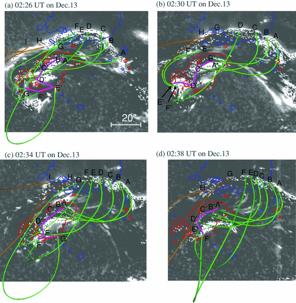
Figure 3. Magnetic field lines and Ca ii image from 02:26 UT to 02:38 UT on 2006 December 13 with the same format as Figure 2. Purple segments connect each footpoint of the NLFF on the positive region. The orange field lines are open lines, which connect to the outside of the analyzed domain on the hybrid magnetogram shown in Figure 1.
Download figure:
Standard image High-resolution imageThis disagreement suggests to us that the reconstruction of the magnetic field in the outer part of the AR is more difficult compared to the inner part near the magnetic neutral line. This might be due to the geometrical influence of the separatrix. In Figure 3, orange lines, e.g., H and I in (a), indicate open field lines, which are connected to the outside of the analyzed domain. The open field lines suggest to us that the separatrix between the closed and open fields might exist in the negative pole. However, we cannot reproduce an accurate structure of the separatrix since the precise location of separatrix is very sensitive to the lateral boundary condition and the iterative procedure of the NLFFF solver. We infer from the results that the lateral boundary condition of our AR model is not accurate enough to reconstruct the structure of the separatrix, and a more sophisticated model should be developed to reproduce the connectivity near the separatrix more accurately.
3.2. Twist of Field Lines
Here, we define the twist of magnetic field line by
where the line integral ∫dl is taken along the magnetic field line. The twist Tn is a function of field lines, and the denominator 4π is introduced so that Tn corresponds to the number of turns of the magnetic field, e.g., Tn = 1 for one turn twist. If the magnetic field is given by a force-free field (Equation (1)),

where L is the length of the magnetic field line, because α is constant along field lines ( ). However, since the value of α derived numerically from magnetograms does not completely guarantee the force-free condition, α at the feet of the field line on positive and negative poles, α+ and α−, do not necessarily have the same value in practical data. In order to reconcile this discrepancy, we adopt the averaged value of α,
In addition, we screen α only in the strong field region, where the normal component Bz of magnetic field exceeds 30 G, and we assume that α = 0 elsewhere in order to avoid the contamination of numerical noise on the weak Bz region in the calculation
where Δ indicates the finite difference. Furthermore, we operate an averaging over 3 × 3 cells on α+ and α−.
Figure 4(a) represents the twist Tn of the field lines tracked from the northern ribbon on four different moments corresponding to the panels of Figure 2. The red crosses mark the twist Tn of field lines rooted to all the pixels on the ribbon, and the black segments A to G are for the selected field lines plotted in Figure 2. The solid line represents the evolution of the averaged value of each moment. It clearly shows that the twist of most of the field lines is negative, corresponding to the left-handed twist. We can also see that the twist is distributed over a wide range for each ribbon and that it tends to be stronger on the western part (in the side near F or G) than the eastern part (in the side near A). Furthermore, the absolute value increased as time passed. This indicates that reconnection of the flare commenced from the inner region rather than the most strongly twisted magnetic arcade.
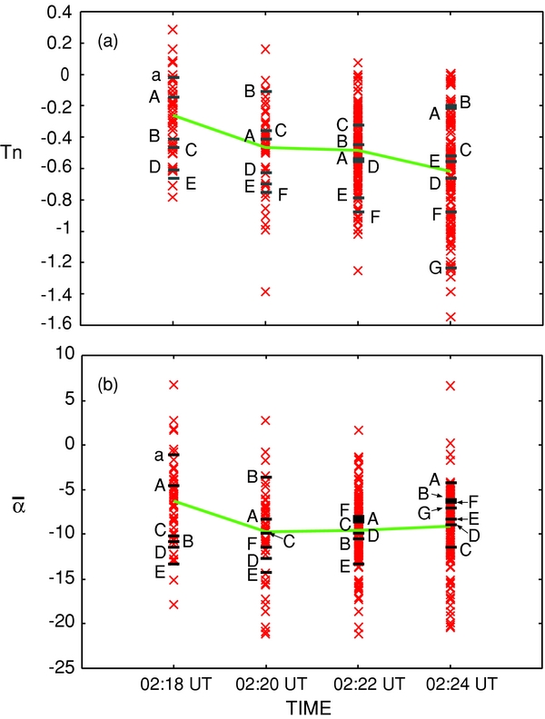
Figure 4. Red crosses represent (a) the twist Tn and (b) the shear parameter  of field lines traced from the ribbons shown in Figure 2. A–G in each time correspond to the selected field lines plotted in Figure 2. The solid green lines connect the average values in each time.
Download figure:
Standard image High-resolution image3.3. Time Evolution of Twisted Flux
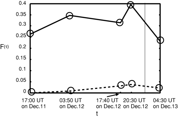
Finally, we study the time evolution of the twisted magnetic flux for about two days before and after the onset of the flare. In Figure 5, we plot the history of the ratio of magnetic flux twisted more than a critical twist τ to the total magnetic flux

where the surface integral is taken on the positive pole Bz > 0 in the region surrounded by the solid square in Figure 1(b).
Figure 5. Time evolution of the fraction of magnetic flux twisted more than τ to the total flux integrated over the square shown in Figure 1. Solid and dashed lines are for τ = 0.5 and 1, respectively. The vertical thin solid line indicates the flare occurring time.
Download figure:
Standard image High-resolution image
We can see that the fraction of a half-turn-twisted flux F(0.5) increased up to 0.4 before the onset of flare (2:10 UT on 2006 December 13), and it drastically decreased to less than 0.25 after the flare (04:30 UT on 2006 December 13). The behavior can be explained well as a consequence of magnetic reconnection in the flare distangling the magnetic twist formed by the counterclockwise rotation of the positive spot. This figure also shows that the fraction of flux twisted by more than one turn F(1) is very small (<0.04), although the tendency in the evolution is similar to the half-turn flux. This result implies that the spot rotation before the flare was not enough to twist a substantial amount of flux to more than one turn, and also that the twist of more than one turn might not necessarily be needed to trigger the onset of the flare. According to Török et al. (2004), the critical twist to destabilize the ideal MHD kink modes in an anchored magnetic loop is about 1.75. Therefore, our result suggests that the ideal MHD instability was hardly relevant to the process triggering the flare.
4. SUMMARY AND DISCUSSION
In this paper, we investigated the connectivity and the twist of magnetic field lines on the flaring AR NOAA 10930 in terms of the NLFFF model extrapolated from time series vector magnetograms. As a result, we have clearly shown that the left-handed twist increased before the onset of the flare, and it quickly decreased after the flare. It is consistent with the store-and-release scenario of magnetic helicity as the basic process of solar flares. Our analysis also revealed that the fraction of magnetic flux that was twisted by more than one turn was small (less than ∼5%), although a substantial amount of magnetic flux was twisted by more than a half turn (∼40%).
Furthermore, we have found that the twist of the field lines connecting to flare ribbons increased as the ribbons were extending outward away from the region near the magnetic polarity inversion line (PIL) in the early phase of the flare. On the other hand, by using Hα observations Asai et al. (2003) showed that the lines connecting the pairs of conjugate footpoints indicated the strong-to-weak shear configuration, and that the sheared angle decreased with the extension of ribbons. However, our analysis of the magnetic twist is not necessarily inconsistent with this previous study, because the twist and the shear are not the same quantities. In Figure 4(b), we show the value of  of each line plotted in Figure 4(a), and we can see that the absolute value of
  tends to decrease weakly with time except for the precise initial moment (2:18 UT), even though the values for each ribbon possess a large scatter. This result is consistent with the previous study, since α is directly related to the sheared angle which Asai et al. (2003) measured.
From these results, we can conclude that magnetic reconnection in a flare may commence from the region where the magnetic field is rather strongly sheared in a magnetic arcade. However, the twist of the first reconnected field is not necessarily highest in the reconnected field. At least in the AR NOAA 10930, the twist of the first reconnected field was smaller than unity and the most strongly twisted region might be located above the first reconnected field lines.
Based on the results above, we infer that the kink mode instability could hardly occur, at least before the onset of the flare, while the strength of the local shear is likely to be relevant to the flare triggering mechanism. For instance, Wang et al. (2008) and Lim et al. (2010) pointed out that some fine structure near the PIL could play a role for the onset of the flare. It is likely that mutual interaction between the large-scale twisted field and the small-scale thin current sheet formed in a highly sheared region leads to the onset of a flare through the nonlinear feedback process (Kusano et al. 2004). However, since the detail dynamics to initiate a flare are still unclear, a careful analysis of the large-scale and small-scale interaction is required. We are currently carrying out more detail analysis, the results of which will be published elsewhere in future.
S.I. thanks Dr. K. Hayashi and Dr. Y. Morikawa for helpful comments and support on this paper. The authors thank Dr. Neel P. Savani for reading the draft paper. The ambiguity resolution code used herein was developed by K. D. Leka, G. Barnes, and A. Crouch with NWRA support from SAO under NASA NNM07AB07C. Hinode is a Japanese mission developed and launched by ISAS/JAXA, with NAOJ as domestic partner and NASA and STFC (UK) as international partners. It is operated by these agencies in cooperation with ESA and NSC (Norway). This work was supported by the Grant-in-Aid for Creative Scientific Research "The Basic Study of Space Weather Prediction" (17GS0208, Head Investigator: K. Shibata), the Grants-in-Aid for Scientific Research (B) "Multi-physics Plasma Dynamics Revealed by Macro-Micro Interlocked Simulations," (19340180, Head Investigator: K. Kusano) and "Understanding and Prediction of Trigger of Solar Flares" (23340045, Head Investigator: K. Kusano) from the Ministry of Education, Science, Sports, Technology, and Culture of Japan. This research was partially supported by Basic Science Research Program (2010-0009258, PI: T. Magara) as well as the WCU (World Class University) program (R31-10016) through the National Research Foundation of Korea. D.S. is supported in part by the Special Postdoctoral Researchers Program at RIKEN. The computational resources, data analysis, and visualization system are supported by the Cybermedia Center Osaka University, and Space Weather Cloud system developed by NICT.