


ABSTRACT
Coherent scattering of limb-darkened radiation is responsible for the generation of the linearly polarized spectrum of the Sun (the Second Solar Spectrum). This Second Solar Spectrum is usually observed near the limb of the Sun, where the polarization amplitudes are largest. At the center of the solar disk the linear polarization is zero for an axially symmetric atmosphere. Any mechanism that breaks the axial symmetry (like the presence of an oriented magnetic field, or resolved inhomogeneities in the atmosphere) can generate a non-zero linear polarization. In the present paper we study the linear polarization near the disk center in a weakly magnetized region, where the axisymmetry is broken. We present polarimetric (I, Q/I, U/I, and V/I) observations of the Ca i 4227 Å line recorded around μ = cos θ = 0.9 (where θ is the heliocentric angle) and a modeling of these observations. The high sensitivity of the instrument (ZIMPOL-3) makes it possible to measure the weak polarimetric signals with great accuracy. The modeling of these high-quality observations requires the solution of the polarized radiative transfer equation in the presence of a magnetic field. For this we use standard one-dimensional model atmospheres. We show that the linear polarization is mainly produced by the Hanle effect (rather than by the transverse Zeeman effect), while the circular polarization is due to the longitudinal Zeeman effect. A unique determination of the full  vector may be achieved when both effects are accounted for. The field strengths required for the simultaneous fitting of Q/I, U/I, and V/I are in the range 10–50 G. The shapes and signs of the Q/I and U/I profiles are highly sensitive to the orientation of the magnetic field.
Export citation and abstract BibTeX RIS
1. INTRODUCTION
Ca i 4227 Å is a preferred line for the exploration of scattering polarization and the determination of the weak magnetic fields in the lower chromosphere (Bianda et al. 1998a, 1998b). This line exhibits the largest degree of linear polarization in the visible spectrum near the limb (Stenflo 1982; Gandorfer 2002; Bianda 2003; Bianda et al. 2003; Sampoorna et al. 2009). A detailed modeling of non-magnetic limb observations of this line has been performed recently by Anusha et al. (2010). The idea of using the Hanle effect near the disk center to measure chromospheric magnetic fields was proposed by Trujillo Bueno (2001). In a one-dimensional axially symmetric atmosphere with no oriented magnetic fields (meaning fields not parallel to the symmetry axis that is the atmospheric normal), the scattering polarization is zero when the line of sight (LOS) is parallel to the atmospheric normal (μ = cos θ = 1, where θ is the heliocentric angle). However, in the presence of an oriented magnetic field, the Hanle effect produces a non-zero scattering polarization. This is usually referred to as the forward-scattering Hanle effect. The first observational evidence for this effect was provided by Trujillo Bueno et al. (2002), who observed it in the He i 10830 Å line. For the Ca i 4227 Å line, Joos (2002) and Stenflo (2003a) showed that the forward-scattering Hanle signatures observed near the disk center (μ = 0.96) can be used for the analysis of weak, horizontal chromospheric magnetic fields. An extensive theoretical study of the linear polarization in the Ca ii IR triplet performed by Manso Sainz & Trujillo Bueno (2010) confirms the usefulness of this effect as a diagnostic tool.
We have performed new full Stokes profile observations of the Ca i 4227 Å line near the disk center, to explore different regions of varying magnetic activity, from very quiet to moderately active. Details of the observations are given in an accompanying paper (Bianda et al. 2011). Here we present an analysis of these observations. The observed circular polarization (V/I) signals indicate that we are observing a solar region with weak longitudinal magnetic flux, which allows us to apply the "weak field approximation" of the Zeeman effect to model the observed V/I profiles (see, e.g., Stenflo 1994; Landi Degl'Innocenti & Landolfi 2004) and thereby determine the longitudinal component of the magnetic flux density. In the weak field approximation V/I is proportional to the derivative of the emergent intensity with respect to wavelength, which can be obtained directly from the observed intensity. Thus the longitudinal component of the vector magnetic flux density is uniquely determined by the observed Stokes V and I, without any model dependence. Since however only one field component is constrained this way, there are multiple solutions (ambiguities) for the field vector itself. When μ ≠ 1 these ambiguities can be eliminated using the observed linear polarization (Q/I and U/I) profiles as additional constraints. When μ = 1 (disk center) these ambiguities cannot be eliminated, because all the Stokes parameters remain unchanged under the transformation χB → χB + π, where χB represents the magnetic field azimuth in the atmospheric co-ordinate system (polar Z-axis along the atmospheric normal).
To model the observed Q/I and U/I profiles the polarized radiative transfer (RT) equation is solved assuming the presence of an oriented vector magnetic field, taking into account partial frequency redistribution (PRD). A standard model atmosphere and a multi-level model atom are used. The solutions at the line center wavelength are used to construct polarization diagrams (i.e., Q/I versus U/I plots; see, e.g., Stenflo 1994). The observed line center data are placed on the polarization diagrams to extract a single vector magnetic field for which the observed and theoretical Q/I and U/I amplitudes at line center agree. Thus the magnetic field values extracted from the V/I profiles with the weak field approximation, together with the Hanle polarization diagrams of Q/I and U/I at the line center, allow us to nicely reproduce the entire wavelength dependence of the observed Q/I, U/I, and V/I profiles. The idea of using a combination of the Zeeman and Hanle effects in magnetic field diagnostics has been explored in several papers in the past (e.g., Bommier et al. 1981; Landi Degl'Innocenti 1982; Ben-Jaffel et al. 2005).
For modeling the observed Q/I and U/I profiles the transverse Zeeman effect can be ruled out for various reasons. (1) The transverse field strengths would have to be more than an order of magnitude stronger than the longitudinal field, implying that all fields would need to "hide" in the transverse plane, which is a very contrived situation. (2) Even then the transverse Zeeman effect is unable to reproduce the Q/I and U/I line shapes with the observed strong π component. (3) The forward-scattering Hanle effect provides a natural explanation of the observed Q/I and U/I, including their profile shapes, with field strengths of the same order as those indicated by the model-independent Stokes V/I fitting for the LOS component.
In Section 2 we briefly describe the theoretical framework of polarized RT used in our calculations. In Section 3, details on the observations are given. Section 4 is devoted to a description of the modeling procedure, where we also give details on the solar atmospheric model, and the model atom. The results and discussions are presented in Section 5. Concluding remarks are given in Section 6.
2. THE RADIATIVE TRANSFER FORMULATION
For our modeling procedure, we have solved non-LTE RT equations for the Hanle effect and for the Zeeman effect but under the weak field approximation.
2.1. Radiative Transfer with the Hanle Effect
2.1.1. Stokes Parameter Formulation
We use the standard notation of line formation theory (Mihalas 1978; Stenflo 1994). The Stokes vector RT equation for a two-level model atom with unpolarized ground level in a one-dimensional planar medium in the presence of weak-field Hanle effect may be written as
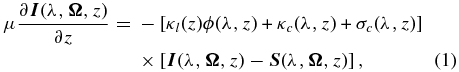
where  = (I, Q, U)T is the Stokes vector and
  the source vector. Here,
  defines the ray direction with θ and φ being the inclination and azimuth of the scattered ray (see Figure 1). The Voigt profile function is denoted by ϕ. The dependence of ϕ on z comes from the damping parameter a = Γtot/4πΔνD. Here

with ΓR being the radiative de-excitation rate. For the Ca i 4227 Å line ΓR = 2.18 × 10⁸ s−1. ΓE and ΓI are the elastic and inelastic collision rates, respectively. ΓE is computed taking into account the van der Waals broadening (arising due to elastic collisions with neutral hydrogen) and Stark broadening (arising due to interactions with free electrons). ΓI includes the inelastic collision processes like collisional de-excitation by electrons and protons, collisional ionization by electrons, and charge exchange processes (see Uitenbroek 2001, and the multi-level atom computer program provided by him). The Doppler width  , where kB is the Boltzmann constant, T is the temperature, Ma is the mass of the atom, vturb is the micro-turbulent velocity (taken as 1 km s−1), and λ0 is the line center wavelength. κl is the wavelength-integrated line absorption coefficient, while σc and κc are the continuum scattering and continuum absorption coefficients, respectively. Other atomic parameters are given in Section 4.1 and Appendix A.
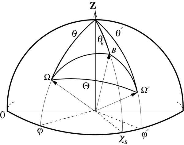
Figure 1. Scattering geometry.  and
and  define, respectively, the directions of the incoming and outgoing beams. Θ is the scattering angle. The Z-axis is along the atmospheric normal.
  defines the orientation of the magnetic field vector.
Download figure:
Standard image High-resolution imageThe total opacity coefficient is κtot(λ, z) = κl(z)ϕ(λ, z) + σc(λ, z) + κc(λ, z). In a two-level model atom with unpolarized ground level, the total source vector  is defined as
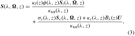
Here,  and Bλ is the Planck function at the line center. The line source vector is
Here,  is the Hanle redistribution matrix (Bommier 1997b).
  is the vector magnetic field taken to be a free parameter. The continuum scattering source vector is
where  is the Rayleigh scattering phase matrix (Chandrasekhar 1960). For simplicity, frequency coherent scattering is assumed for the continuum. The thermalization parameter
  is defined by = ΓI/(ΓR + ΓI). In Equation (4) (λ',
  ) and (λ,
  ) refer to the wavelength and direction of the incoming and the outgoing rays, respectively.
2.1.2. Spherical Irreducible Tensor Decomposition
In general the Stokes source vector  and the Stokes vector
  in Equation (1) depend on
  . As shown in Frisch (2007), the vectors
  and
and  can be decomposed into six cylindrically symmetric components,
  and
and  , with K = 0, 2 and Q ∈ [ − K, +K], if one represents them in terms of the spherical irreducible tensors for polarimetry defined in, e.g., Landi Degl'Innocenti & Landolfi (2004). With these components one can construct an irreducible source vector
  and an irreducible Stokes vector
  . This decomposition is useful because
  becomes independent of the ray direction and
  becomes independent of the azimuthal angle φ. The transfer equation for
  may be written as
In a two-level model atom with unpolarized ground level, the total irreducible source vector  is defined as
Here,  . The irreducible line source vector is
Here, μ' represents the incoming ray direction. The irreducible polarized continuum scattering source vector is
 is the angle-averaged PRD matrix in the irreducible basis for the Hanle effect (see Bommier 1997a, 1997b) given in Equation (A1) of Appendix A. The matrix
  is the Rayleigh scattering phase matrix in the irreducible basis. Its elements are given in Appendix A of Frisch (2007; see also Faurobert-Scholl 1991). We define the total optical depth scale through dτλ = −κtot(λ, z)dz.
The formal solution of Equation (6) can be written as
for μ > 0, and
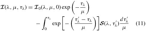
for μ < 0.  represents a radiation field that is incident on the medium. We assume that no radiation is incident on the upper free boundary (τλ = 0), while at the lower boundary Tλ,
  .
.
The redistribution matrices used here are defined under the approximation III of Bommier (1997b; see our Appendix A). We take into account the depth dependence of the branching ratios that appear in the redistribution matrix  , in contrast to Nagendra et al. (2002) and Fluri et al. (2003), where these coefficients were kept independent of depth, because only isothermal atmospheres were considered. The polarized Hanle RT equation is solved for the irreducible Stokes vector
  . The Stokes vector (I, Q, U)T can then be deduced from
  (see, e.g., Frisch 2007; Anusha & Nagendra 2011). The components of
  are (I00, I20, I2x1, I2y1, I2x2, I2y2). If the magnetic field is zero, or micro-turbulent, only the two components I00 and I20 are non-zero. It is easy to see from the expression of Stokes Q that Q = 0 at the disk-center (μ = 1) and maximum at the limb (μ = 0) and that U = 0. The same argument applies to S00 and S20. When the magnetic field is non-zero and has some fixed orientation, then all six components are non-zero. Therefore, Stokes Q will be non-zero at the disk center and U will be non-zero with contributions coming from the four components I2x1, I2y1, I2x2, I2y2. This is what is referred to as the forward-scattering Hanle effect.
2.2. Radiative Transfer with the Zeeman Effect
The non-LTE Zeeman-effect line transfer equation for the Stokes vector (I, Q, U, V)T is given by
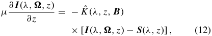
where  is the absorption matrix. In Appendix B we give the relevant trigonometric functions that are required to write the Zeeman absorption matrix in the atmospheric reference frame. The general form of
  for a multi-level model atom can be found in Landi Degl'Innocenti & Landolfi (2004).
We recall that Equation (1) is the Hanle RT equation written for the Stokes parameters (I, Q, U)T (Stokes V is not included because it is not generated by the weak-field Hanle effect). Stokes I is not very sensitive to the magnetic field in the weak field limit (see Equation (13) below). Equation (12) is the Zeeman RT equation written for the Stokes vector (I, Q, U, V)T. The Stokes parameters Q and U appearing in Equations (1) and (12) are the same quantities. In Equation (1) the Stokes Q is generated by resonance scattering but modified by a weak magnetic field  , while Stokes U is generated entirely by the Hanle effect. In Equation (12) Stokes Q and U are generated by the transverse Zeeman effect. However, for the range of fields indicated by the observed V/I amplitudes (see below), Stokes Q and U generated from the transverse Zeeman effect are negligible, and therefore Stokes V decouples from Stokes Q and U in Equation (12). Further, we assume that the amount of atomic polarization in the upper level of the line is weak (due to the small value of the anisotropy of the solar radiation field). Thus, under this approximation combined with the weak field limit the RT equation for the linear polarization (Equation (1)) decouples from the RT equation for the circular polarization (Equation (12)). With the assumption of height independent magnetic fields the weak field approximation (see, e.g., Stenflo 1994; Landi Degl'Innocenti & Landolfi 2004) is defined as
where

with geff being the effective Landé factor (geff = 1 for the Ca i 4227 Å line). The line center wavelength λ0 is given in Å and B in Gauss. ΔλD is the Doppler width expressed in wavelength units.
For the Ca i atom ΔλD = 31 mÅ at the top of the FALC model atmosphere (where T = 9257 K). For the Ca i 4227 Å line we get ΔλH = 8.33487 × 10⁻³B. The Zeeman splitting equals the Doppler width for a field strength of about B = 3720 G . In Table 1 we list the ratio ΔλH/ΔλD for various B values. For B ⩽ 40 G, we have ΔλH/ΔλD ⩽ 1%, so for B ⩾ 50 G the ratio ΔλH/ΔλD starts to become significant.
Table 1. List of the Ratio ΔλH/ΔλD for Various B Values
| B | ΔλH/ΔλD |
|---|---|
| 10 | 0.003 |
| 20 | 0.005 |
| 30 | 0.008 |
| 40 | 0.010 |
| 50 | 0.013 |
| 60 | 0.016 |
| 70 | 0.019 |
| 80 | 0.022 |
| 90 | 0.024 |
| 100 | 0.027 |
| 500 | 0.134 |
| 1000 | 0.269 |
| 2000 | 0.538 |
| 3000 | 0.807 |
Download table as: ASCIITypeset image
Under the weak field approximation (Equation (13)) V/I is simply given by
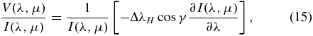
where I(λ, μ) is the emergent Stokes I profile, and

Here, B, θB, and χB represent the strength, inclination, and azimuth of the magnetic field vector (see Figure 1). In all our calculations we set φ = 0° and cos θ = μ = 0.9. Use of Equation (15) allows us to bypass the numerically expensive task of solving the Zeeman RT equation for a range of B, θB, and χB values.
3. OBSERVATIONS OF I, Q/I, U/I, AND V/I IN THE Ca i 4227 Å LINE
The data acquisition was done with the ZIMPOL-3 polarimeter (Ramelli et al. 2010) at IRSOL in Switzerland. More observational details are given in Bianda et al. (2011). The observations were obtained on 2010 October 15 near the active solar region NOAA 1112 (S19 W5). Figure 2 shows the position of the spectrograph slit, which was 60 μm wide (0.5 arcsec on the disk) and subtended 184 arcsec. The slit orientation was parallel to the geographical north limb. The resulting CCD images are 140 pixels high in the spatial direction, with a pixel corresponding to 1.3 arcsec, and 1240 pixels wide in the wavelength direction, with a pixel corresponding to 5.3 mÅ. The total exposure time was about 8 minutes (500 single recordings of 1 s each). These observations correspond to an average μ value of 0.93. Note that μ values determined for near disk center observations are more accurate compared to those determined near the limb. Figure 3 shows the CCD image of the Ca i 4227 Å line. From the Stokes profiles in Figures 7–10 we can see that the orders of magnitude of the observed Q/I, U/I, and V/I are in the range 0.1%–1%. This indicates that the observed regions are weakly magnetized. We have selected a set of eight observed Stokes profiles for analysis. Each of these profiles is a result of averaging over three to four pixels along the slit (to reduce noise). These eight profiles represent different spatial locations on the solar disk and therefore are expected to have different magnetic fields. Henceforward these eight locations are referred to as locations (or observation points) 1–8. Other near disk center observations have been performed at IRSOL. They can be modeled with the same strategy.
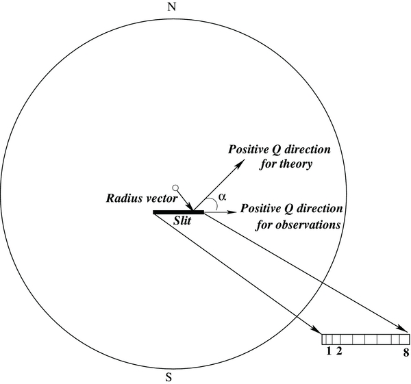
Figure 2. Slit position on the solar disk and the definition of the rotation angle α. The numbers 1, 2, ..., 8 represent eight positions within the slit, from which the spatially averaged observed profiles are extracted for the theoretical modeling. The average value of μ corresponding to the slit position is 0.93. The positive Q direction for the theoretical calculations is defined to be perpendicular to the radius vector.
Download figure:
Standard image High-resolution image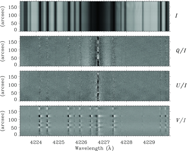
Figure 3. CCD image of the Stokes parameters in a spectral window around the Ca i 4227 Å line. The recording was made on 2010 October 15. See Section 3 for more details.
Download figure:
Standard image High-resolution imageThe positive Q/I direction for the observations is defined to be parallel to the slit direction (or parallel to the geographical north limb), whereas the positive Q/I direction for the RT problem is defined to be perpendicular to the radius vector. For each point on the slit, the observational data must therefore be converted to the system where positive Q/I is oriented perpendicular to the solar radius passing through this point (see Figure 2). So for each point, if (Q', U')T denotes the original observed data, (Q, U)T for a system where positive Q/I is oriented perpendicular to the solar radius is given by
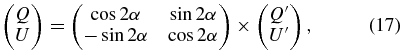
where α is the angle between the slit direction and the vector perpendicular to the radius vector (see Figure 2).
We note that Stokes I and V are unaffected by the rotation angle α (see Equation (13.3) of Stenflo 1994).
Spectropolarimetric observations of the Ca i 4227 Å line at the limb have revealed wing polarization anomalies (see Bianda et al. 2003; Nagendra et al. 2002, 2003; Sampoorna et al. 2009), which have been referred to as the "wing Hanle effect enigma." The work of Sampoorna et al. (2009) has shown that according to the best theoretical approaches now available, it is impossible to explain these wing anomalies in terms of the Hanle effect, and therefore alternative mechanisms have been qualitatively invoked. The wing Hanle effect enigma basically means that the signals that are measured close to the limb are characterized by a faint depolarization in the Q/I wings, while the U/I wings exhibit Q/I like shapes, with amplitudes that are small fractions of the Q/I amplitudes. Our observations indicate that while the signals can be easily found near the solar limb, they quickly become rare when moving toward the disk center. All the polarization effects that we observe and try to model near the disk center for the forward-scattering Hanle effect are concentrated in the inner wings, near the line core, while the wing anomalies observed near the limb would be located significantly further out, in the outer wing region. As we do not observe any polarization effects near the disk center in these outer wing regions, neither in Q/I, nor in U/I, all that we are dealing with in the forward-scattering case has nothing to do with the wing Hanle effect enigma; it is an entirely unrelated phenomenon.
4. MODELING PROCEDURE
The theoretical polarized spectrum is calculated using a two-stage process similar to the one described in Holzreuter et al. (2005). In the first stage a multi-level PRD-capable MALI (Multi-level Approximate Lambda Iteration) code of Uitenbroek (2001, hereafter called the RH-code) solves the statistical equilibrium equation and the unpolarized RT equation self-consistently and iteratively. The RH-code is used to compute the intensity, opacities, and the collision rates. In the second stage, the opacities and the collision rates are kept fixed, and the vector  is computed perturbatively by solving the polarized Hanle transfer equation. The Stokes vector
  can then be deduced using the irreducible vector
  . For simplicity, in the second stage a two-level atomic model is assumed for the particular transition of interest.
In the present paper the RT equations are solved for μ = 0.9. We have verified that one can retain this single μ value to analyze all the observation points along the slit. The vector magnetic field  is a free parameter. In all the calculations
  is assumed to be uniform with height. We also assume that it is filling all the space for reasons that are explained in Section 5.6. Our modeling procedure can be described in three steps (see Sections 4.2–4.4).
4.1. The Model Atmosphere and the Model Atom
We use the FALC model atmosphere (Fontenla et al. 1993), which we find to be better for reproducing the observed linear polarization profiles from the Hanle effect. For comparison we also show theoretical profiles computed with the FALX model atmosphere (Avrett 1995; see our Figure 11).
In the multi-level RH-code, the atomic model of Ca i consists of 20 levels, with 17 line transitions and 19 continuum transitions. The main line is treated in PRD, using the angle-averaged PRD functions of Hummer (1962). All other lines of the multiplet are treated in complete frequency redistribution (CRD). However, for computing the polarization we restrict ourselves to a two-level atom model for the main line transition. All the blend lines are assumed to be depolarizing. They are treated in LTE in the RH-code. Therefore, the blend line absorption coefficient is implicitly included in the continuum absorption coefficient κc.
4.2. Step 1. Polarization Profiles for V/I
In this step we first derive the value of Bcos γ (longitudinal component) that is uniquely determined by the observed V/I profile when compared with the derivative of the observed Stokes I profile (see Equation (15)). We then compute ensembles of B, θB, and χB values that all reproduce the uniquely determined Bcos γ. These ensembles are model independent because they are directly based on the observed V/I and I profiles. For more details see Section 5.1.
4.3. Step 2. Polarization Diagrams for Q/I and U/I at the Line Center
While Step 1 fixes the value of the LOS component of  by using Stokes V, the components in the transversal plane are entirely unconstrained. To determine all three components of the field vector we need two additional observables, namely, the observed Q/I and U/I. We generate theoretical polarization diagrams for Q/I and U/I at the line center computed using the RT equation with the Hanle effect (see Equation (1)) for the sets of
  values already extracted in Step 1. The observed line center values of Q/I and U/I are marked on these diagrams. With the polarization diagrams we can remove the ambiguities in the B, θB, and χB values. For more details see Section 5.2.
4.4. Step 3. Polarization Profiles for Q/I and U/I
In this step we compare the observed profiles with the theoretical profiles calculated with the B, θB, and χB values extracted from Steps 1 and 2. Although in Step 2 we use the Q/I and U/I values only at line center, it turns out that these B, θB, and χB values are also able to reproduce the wavelength dependence of the observed Q/I and U/I profiles in the line core. For more details see Section 5.3.
5. RESULTS AND DISCUSSION
In this section we discuss the results of the modeling procedure described in the previous section.
5.1. V/I Profiles from the Zeeman Effect
Here we discuss in more detail how Step 1 is performed (Section 4.2). For the computation of the V/I profiles in Step 1 using Equation (15) we consider a grid of magnetic field parameters B, θB, and χB, which are in the range B ∈ [0 G, 50 G] in steps of 5 G, θB ∈ [0°, 180°] in steps of 5°, and χB ∈ [0°, 360°] in steps of 11 25. For the computation of the derivative of the intensity with respect to the wavelength in Equation (15) we use the observed Stokes I itself. For differentiation we use an in-built subroutine (in the IDL programming language) that performs a numerical differentiation using a three-point Lagrangian interpolation. For a given location and a given field strength, we get several sets of (θB, χB) values (a minimum of 0 to a maximum of 120 sets) consistent with the observed V/I profiles.6 The field strengths derived here always correspond to weak values of B (10 G–50 G), consistent with the fact that the observed V/I signals are in the range 0.1%–0.9%. We have investigated the behavior of the V/I profiles in the full range of B ∈ [0 G, 50 G], θB ∈ [0°, 180°]. For each observation point the V/I model fitting restricts the values of B and θB to be, respectively, in the smaller sub-intervals of [0 G, 50 G] and [0°, 180°]. No such restriction is imposed on the χB values.
5.2. Polarization Diagrams from the Hanle Effect
The values of B, θB, and χB deduced from Stokes V should also fit the observed Q/I and U/I profiles. For field strengths below a few hundred G the transverse Zeeman effect does not produce any significant Q/I and U/I. In contrast, at these field strengths, the Hanle effect plays an important role: it modifies the Q/I generated by the resonance scattering and creates a non-zero U/I. Hence, Q/I and U/I provide constraints on the magnetic field vector which are independent of those stemming from V/I. We compute the theoretical Stokes profiles (I, Q/I, and U/I) considering only the Hanle effect (see Equation (1)) with B, θB, and χB in the range restricted by the V/I model fitting. Since in the weak field approximation the transfer equation for Stokes V decouples from the transfer equation for (I, Q, U)T, Hanle scattering does not produce any V/I signal unless there exists an initial source of the circular polarization.
We recall that the polarization diagrams are plots of Q/I versus U/I for given values of field strength B, wavelength λ, and LOS defined by μ, φ (see, e.g., Bommier 1977; Landi Degl'Innocenti 1982; Bommier et al. 1991; Faurobert-Scholl 1992; Stenflo 1994; Nagendra et al. 1998). The values of θB and χB are varied in finite steps. A closed curve (hereafter loop) is produced in the (Q/I, U/I) plane as χB is varied from 0° to 360°. Each value of θB corresponds to a different loop. The size and tilt of the polarization pattern in a loop with respect to the vertical (Q/I = 0 line) depend on the value of B and θB. Examples of polarization diagrams are shown in Figures 4 and 5 for B = 10 G, 15 G, 30 G, and 50 G. They are constructed with the theoretical Q/I and U/I values at line center calculated with μ = 0.9 and φ = 0°. Different loops correspond to different values of θB ∈ [100°, 175°], incremented in steps of 5°. In each of the loops the small square symbol corresponds to the first grid point χB = 0°, and as we proceed in the counterclockwise direction, χB takes values between 0 and 360 in steps of 11.25 deg.

Figure 4. Polarization diagrams for two values of B (10 G, 15 G), θB ∈ [100°, 125°], χB ∈ [0°, 360°], for μ = 0.9, and at line center. The solid, dotted, dashed, dot-dashed, triple-dot-dashed, and long dashed lines of the loops, respectively, correspond to θB = (100°, 105°, 110°, 115°, 120°, and 125°) in panels (a) and (b). The points corresponding to χB = 0 are marked by small square symbols. We move along the curves in the counterclockwise direction as χB is increased from 0° to 360°. The line center observations of Q/I and U/I are marked as big squares-i, where i = 1,... , 8 stand for eight locations on the slit. The observations were done on 2010 October 15.
Download figure:
Standard image High-resolution image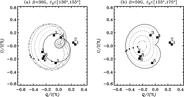
Figure 5. Same as Figure 4, but for the values of the field strength B = 30 G (panel (a)) and B = 50 G (panel (b)). The solid, dotted, dashed, dot-dashed, triple-dot-dashed, and long dashed lines of the loops, respectively, correspond to θB = (130°, 135°, 140°, 145°, 150°, and 155°) in panel (a) and θB = (155°, 160°, 165°, 170°, and 175°) in panel (b).
Download figure:
Standard image High-resolution imageThe observed Q/I and U/I at the line center, averaged over three pixels in the wavelength domain (in order to reduce noise) are marked in the diagrams as big squares-i, where i = 1,... , 8 stand for the eight locations on the slit. We recall that we refer to these eight locations as observation points 1–8.
We find that among the different solution sets (B, θB, and χB) given by the weak field approximation of the Zeeman effect, there is only one choice which can simultaneously fit the observed line center values of Q/I and U/I.
Our results strongly suggest that observed Q/I and U/I are signatures of the Hanle effect and V/I of the Zeeman effect. Whether resolved inhomogeneities in the atmosphere and velocity fields also contribute to the linear and circular polarizations is a question which goes far beyond the scope of this paper.
In Figure 7 we show the Q/I, U/I, and V/I fits for the observation points 1 and 2. The best fit values of the vector magnetic field for these points are (B, θB, χB) = (15 G, 125°, 56°) and (B, θB, χB) = (15 G, 110°, 191°), respectively. Figures 8–10 are similar to Figure 7, but for the observation points 3–8.
5.3. Q/I and U/I Profiles from the Hanle Effect
It can be observed on the CCD image shown in Figure 3 and on the observed spectra shown in Figures 7–10 that the shapes and signs of the Q/I and U/I profiles in the line core region vary significantly along the slit. These variations can be ascribed predominantly to changes in the magnetic field direction. In Figure 6 we show how sensitive indeed are the cores of Q/I and U/I profiles to the values of θB and χB. We also find that the values of B, θB, and χB, which give the best fits to the line center values of the observed Q/I and U/I, also give the best fits to the observed Q/I and U/I at other wavelengths in the line core. The most likely reason is that the frequency dependence of the line core polarization is essentially controlled by the anisotropy of the radiation field. In the wings, the values of U/I tend to zero and those of Q/I are controlled by Rayleigh scattering and PRD effects. A comparison of I, Q/I, and U/I profiles formed under CRD and PRD mechanisms are presented in Figure 7. See Appendix A for the definition of CRD. In the left panel, we compare the theoretical profiles of Q/I calculated with PRD (thick solid lines) and CRD (thin solid lines) for the observation point 1. This figure clearly shows that the wing shapes and peak values can be nicely fitted with PRD but not with CRD. Also note that the line center values of Q/I and U/I computed with CRD are smaller than those computed with PRD (by about 15% in terms of relative difference in Q/I). Moreover, we find that with CRD we are unable to reproduce the line center values of Q/I and U/I, for many of the observation points on the slit. Indeed, most of the observed values of Q/I and U/I lie outside the polarization diagrams constructed with CRD. Our results clearly show that PRD effects need to be taken into account in the determination of the magnetic field from the Ca i 4227 Å line polarization. The analysis of the second solar spectrum by Belluzzi & Landi Degl'Innocenti (2009) suggests that this conclusion could also hold for many other lines.

Figure 6. Illustration of the sensitivity of the Q/I and U/I profiles to the magnetic field orientation. Panel (a) shows the dependence of the Q/I and U/I profiles on θB for a fixed value of χB = 55°. Solid, dotted, dashed, dot-dashed, and triple-dot-dashed curves represent θB = 5°, 30°, 60°, 70°, and 90°, respectively. Panel (b) shows the dependence of Q/I and U/I profiles on χB for a fixed value of θB = 80°. Thick solid, dotted, dashed, dot-dashed, triple-dot-dashed, long dashed, and thin solid curves represent χB = 11°, 34°, 56°, 68°, 79°, 101°, and 113°, respectively.
Download figure:
Standard image High-resolution image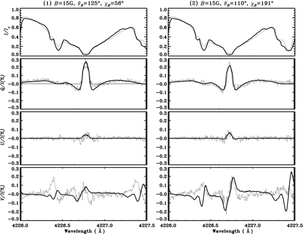
Figure 7. Illustration of the best fit of the theoretical model profiles (solid lines) to the observed profiles (dotted lines) for the observation points 1 (on the left panels) and 2 (on the right panels). The theoretical Q/I and U/I profiles are computed from the Hanle effect and the V/I profiles from the weak field approximation of the Zeeman effect. In the left panels, the thin solid lines represent the profiles computed under the assumption of CRD. The observed V/I profiles show signatures in the wings that are due to Fe blend lines, but here we model only the V/I that is generated by the Ca i 4227 Å line.
Download figure:
Standard image High-resolution image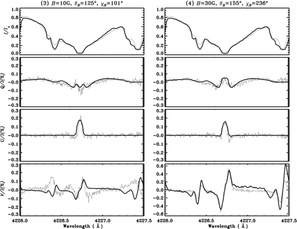
Figure 8. Same as Figure 7 but for the observation points 3 and 4.
Download figure:
Standard image High-resolution image
Figure 9. Same as Figure 7 but for the observation points 5 and 6.
Download figure:
Standard image High-resolution image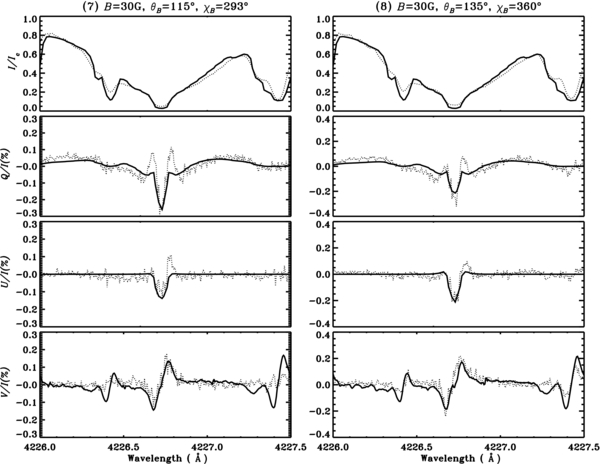
Figure 10. Same as Figure 7 but for the observation points 7 and 8.
Download figure:
Standard image High-resolution imageWe note here that the irreducible components  , Q ≠ 0, only contribute to the line cores of Q/I and U/I, because they are created by the Hanle effect. The component
  on the other hand contributes to both the line core and the wings, but for Q/I alone.
5.4. The Effect of Model Atmospheres
In the left panels of Figure 10 we see positive peaks in the observed profiles of Q/I at 4226.65 Å and in both Q/I and U/I at 4226.8 Å (region of core minima). We have explored the possibility that these peaks could be due to the transverse Zeeman effect. Although these peaks can well be explained in terms of the σ components of the transverse Zeeman effect (but with fields much stronger than the range indicated by the observed Stokes V), it is not possible to fit the core peaks in terms of the π component of the transverse Zeeman effect. Only scattering and the Hanle effect can generate core signatures of sufficient amplitude in the linear polarization. This fact can be seen in Figure 11(a), where we compare the theoretical Stokes profiles computed using the Zeeman effect (using the RH-code) and the Hanle effect with the observational point 7. The  values used for the profiles computed using the Hanle effect are (30 G, 115°, 293°) and those computed using the Zeeman effect are (100 G, 90°, 203°). The curves showing the fit from the Hanle effect are the same as in the left panel of Figure 10.

Figure 11. Panel (a) shows a comparison of the theoretical Stokes profiles (I/Ic, Q/I, and U/I) computed with the Hanle effect (solid lines) and the Zeeman effect (dashed lines) with the observations (dotted lines) for the observational point 7. The  values used for the profiles computed using the Hanle effect and the Zeeman effect are, respectively, (30 G, 115°, 293°) and (100 G, 90°, 203°). The V/I profiles for these two magnetic field configurations computed using the weak field approximation of the Zeeman effect are shown as solid and dashed lines, respectively. Panel (b) shows a comparison of model profiles (I/Ic, Q/I, and U/I) computed using two model atmospheres, FALC (solid lines) and FALX (dashed lines), with the observational data (dotted lines) for the observation point 7. The B and θB values for the FALC and FALX model atmospheres are the same, while the χB values are 293° and 315°, respectively. The V/I profiles for these two magnetic field configurations computed using the weak field approximation of the Zeeman effect are shown as solid and dashed lines, respectively.
Download figure:
Standard image High-resolution imageAnother explanation of the mentioned peaks could be in terms of a different temperature structure of the atmosphere. To verify this we have tested a cooler model atmosphere (FALX). While the FALX model can generate these peaks, it fails to reproduce the observed line center Q/I and U/I amplitudes. The FALC model on the other hand can reproduce the line center peaks but not the peaks near the region of core minima. These results are shown in Figure 11(b), where we compare the theoretical Stokes profiles computed with the FALC and FALX model atmospheres, which give the best fit to the observation point 7. The FALC fit is the same as the one in the left panel of Figure 10. The  values derived from the FALC and FALX model atmospheres are, respectively, (30 G, 115°, 293°) and (30 G, 115°, 315°). We note that the two model atmospheres give two different azimuths χB. However, the FALC model gives an overall better fit than the FALX model. For all other observation points we find that FALX cannot reproduce the line center peaks, and that the overall fit is better in terms of the FALC model. Therefore, we have chosen the FALC model for all our calculations in the present paper.
We note that the positive red and blue peaks in the left panels of Figure 10 are asymmetric in nature. These differences between the red and the blue peaks in the observed Q/I and U/I profiles cannot be interpreted in terms of the Hanle effect, the transverse Zeeman effect, or a different temperature structure. This is because our theoretical profiles always produce symmetric red and blue peaks. In reality we observe such asymmetries often in Stokes spectra, and it is well known that they are due to spatially unresolved, correlated gradients of the magnetic and velocity fields in the solar atmosphere (see Stenflo et al. 1984; Stenflo 2010). However we have not taken up such studies in the present paper.
In Anusha et al. (2010) we found that the FALX model atmosphere gave a better fit to the observed profiles when modeling the non-magnetic limb observations of the Ca i 4227 Å line, while our present disk-center work favors the FALC model. In Figure 12(a) we compare the I/Ic, Q/I profiles computed using FALC and FALX model atmospheres for μ = 0.1 with the observations. We need three free parameters to model the non-magnetic observations. They are (1) an enhancement parameter c, associated with the elastic collision rate ΓE, vW (of the van der Waals type), (2) a global scaling parameter s, and (3) a micro-turbulent magnetic field Bturb (see Anusha et al. 2010, for more details). One can notice that with a proper choice of free parameters FALX gives a better fit than the FALC model atmosphere to the non-magnetic limb observations of the Q/I profiles. This indicates that the actual temperature structure in the solar atmosphere might be better represented by a combination of model atmospheres (two-component models), but such studies are outside the scope of the present paper.
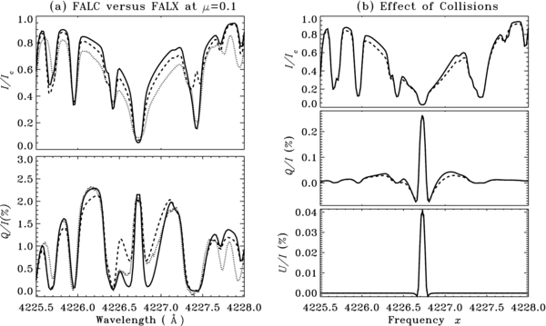
Figure 12. Panel (a) shows comparison of I/Ic and Q/I profiles for μ = 0.1 and for the FALC (solid lines), FALX (dashed lines) model atmospheres with the observations (dotted lines). Two of the three free parameters for FALC and FALX model atmospheres are the same, namely, c = 1.5, s = 1.8. Bturb = 25 G for FALC and Bturb = 30 G for FALX. Panel (b) shows the effect of ΓE, vW on the Q/I and U/I profiles computed for μ = 0.9 for the FALC model atmosphere. We have used c = 1 and c = 1.5 for solid and dashed lines, respectively. The magnetic field values are (B, θB, χB) = (15 G, 125°, 56°).
Download figure:
Standard image High-resolution image5.5. The Role of Collisions
The depolarizing effect of a magnetic field is often mimicked by a similar effect due to collisions and, in many cases, it is difficult to disentangle the two effects. In this paper we assume that the main contribution to the elastic collisions come from the van der Waals type collisions (ΓE, vW). In Anusha et al. (2010) we found that in fitting the limb observations, particularly in reproducing asymmetric Q/I wing shapes, an enhancement of ΓE, vW by a factor of c = 1.5 became necessary. A similar enhancement was also applied by Faurobert-Scholl (1992) to fit the observed Q/I wing polarization. The justification for this can be found in Derouich et al. (2003) and Barklem & O'Mara (1997), who respectively show that the old theories for the depolarizing elastic collision rate D(2) and line broadening elastic collision rate ΓE actually underestimate ΓE, vW.
However, in the present paper, in fitting the near disk center observations we are able to reproduce the wing shapes of Q/I without any enhancement of ΓE, vW. We examine the effect of such an enhancement of ΓE, vW by taking c = 1.5 in Figure 12(b). It is clear that the differences arising due to this effect are small and the effect is mainly in the wings of the Q/I profiles, which are insensitive to the magnetic fields. The line core is unaffected by this modification of ΓE, vW, because the line core is formed higher in the atmosphere where elastic collisions do not play any significant role. Thus our magnetic field determinations are unaffected by the inconsistencies in the theories for the elastic collision rates.
5.6. The Role of a Filling Factor
When interpreting Zeeman-effect observations of photospheric magnetic fields it is generally necessary to introduce a filling factor as a free parameter, since photospheric fields are extremely intermittent, with most of the flux in the form of strong (kG) elements occupying typically only 1% of the quiet photosphere (Stenflo 1973). The introduction of a filling factor as an additional free model parameter opens up a family of new solutions, which is destructive of the uniqueness of the solution unless some appropriate additional observational constraint is brought in. In the case of the photospheric Zeeman effect, the crucial additional constraint has been the introduction of the Stokes V line ratio, using simultaneous observations in two spectral lines that are formed in the same way but differ in their Landé factors.
Adding a magnetic filling factor as an additional degree of freedom in our interpretations of the Hanle forward-scattering observations might therefore seem to open up a Pandora's box of new possibilities, for which we, with our single-line observations, have no useful constraint. The actual situation is however not at all as unconstrained as it may seem earlier, since there are good reasons to believe that the filling factor is close to unity in our case and therefore does not play the role that it does in photospheric Zeeman-effect observations.
The argument for this is as follows: many of our observed polarization amplitudes in the core of the 4227 Å line are so large that theoretical modeling with the FALX atmosphere is unable to produce sufficient polarization, although the implicitly assumed filling factor is the maximum of 100%. Only with a hot atmosphere like FALC does a fit become possible. With any other filling factor the theoretically predicted polarization amplitudes will be smaller, in proportion to the assumed filling factor. This simply brings the observed amplitudes out of reach for a fit. Only with a filling factor close to unity is a fit at all possible in many of the observed cases.
In the case of the photospheric Zeeman-effect observations the situation is very different. The observed polarization amplitudes are mostly very small (on the quiet Sun). Since there is proportionality between circular polarization and field strength over a very wide range, from zero to typically about 500 G, where saturation gradually begins to set in, a tiny filling factor can easily be compensated for by a large field strength to fit the observed polarizations. With the line ratio (determining the differential Zeeman-effect nonlinearity between the two lines) the value of the field strength can be fixed. In contrast to the Zeeman-effect case, however, the Hanle polarization effects do not scale in proportion to the field strength. A small filling factor therefore cannot be compensated for by a large field strength or by any other field parameter, both because the field dependence is very nonlinear, and saturation takes place already for rather weak fields.
The question may then arise why we here conclude that the filling factor must be close to unity, while with Zeeman-effect observations we are used to filling factors that are a couple of orders of magnitude smaller. There are two reasons for this.
The first reason is that our 4227 Å observations refer to the chromosphere, and it is well known that the behavior of the Hanle effect in photospheric lines (like Sr i 4607 Å) and chromospheric lines (like Ca i 4227 Å) is entirely different (Stenflo 2003b). While the photospheric lines do not show much of any spatial structure and rarely any trace of a Stokes U signal, the chromospheric lines are full of spatial structures along the slit in both Q and U. The absence of U signals in the photospheric lines can be understood in terms of tangled fields on scales much smaller than the spatial resolution element, causing cancellation of the positive and negative contributions to Stokes U over each resolution element. The circumstance that we see substantial polarization signals in Stokes U with no evidence for cancellation effects in the chromospheric lines is evidence for resolved fields (filling factor near unity).
The second reason is that the 4227 Å observations that we are trying to fit here do not represent entirely quiet regions on the Sun, but were recorded in the outskirts of active regions, where we found an abundance of clear forward-scattering polarization signatures. In contrast, much less polarization is found far from active regions. The filling-factor concept may be more applicable in such truly quiet regions, but there the signals are so small that they are hard to measure with any acceptable signal-to-noise ratio. Application of the forward-scattering Hanle effect to quiet regions is therefore presently out of reach for two reasons: insufficient signal-to-noise ratio of the observations, and insufficient observational constraints (with single-line observations) when the fields are not spatially resolved.
6. CONCLUDING REMARKS
We have analyzed spectropolarimetric observations of the Ca i 4227 Å line obtained near the center of the solar disk (μ = 0.93). The use of ZIMPOL-3 allows us to attain the required polarimetric precision. We analyze eight positions along the slit, which represent different magnetic fields. These high-quality observations are modeled in three steps.
In the first step we use the weak field approximation of the Zeeman effect as applied to the V/I profiles. We use Equation (15) to compute the V/I profiles with (B, θB, χB) as a free parameter. We extract the values of (B, θB, χB), all of which represent the identical value of Bcos γ (the longitudinal component of  ) that has been fixed by the observed V/I. For each observation data point we obtain a large set of (B, θB, χB) values, which give equally good fits. In the second step we solve the polarized Hanle RT equation (Equation (1)) for the Stokes parameters (I, Q, U)T. The parametric space covered in this step is restricted to the values of (B, θB, χB) already extracted from the V/I model fitting. We construct polarization diagrams of Q/I versus U/I at the line center and mark the "observed" line center data points on these diagrams. With the polarization diagrams we find that only one among the set of (B, θB, χB) values obtained from the V/I model fitting is able to reproduce the observed Q/I and U/I at the line center. In the third step we analyze the shapes of the Q/I and U/I profiles in the line core region. It turns out that the
  values that give good fits to the observations at the line center also reproduce the entire wavelength dependence of the observed Q/I and U/I.
The vector magnetic field constitutes three independent free parameters B, θB, and χB. We have three constraints, namely, the Q/I and U/I profiles generated mainly by scattering and the Hanle effect, and the V/I profile generated by the longitudinal Zeeman effect. Through a combined modeling that uses the Zeeman effect (Step 1) and the Hanle effect (Steps 2 and 3), we have been able to fit, with a single choice of  , the three profiles (Q/I, U/I, and V/I) for the eight observed locations that we have analyzed. In Table 2 we list these (B, θB, χB) values for the eight observed profiles. The extracted field strengths are weak, namely, B ∈ [10 G, 50 G]. The average θB is 136°. The values of χB are quite random. The Stokes I profile is not greatly affected by the range of field strengths that we are interested in (10–50 G).
Table 2. The Values of B, θB, and χB Derived from the Model Fits to the Observed Q/I, U/I, and V/I Data Sets
| Observation point | 1 | 2 | 3 | 4 | 5 | 6 | 7 | 8 |
|---|---|---|---|---|---|---|---|---|
| B (G) | 15 | 15 | 10 | 30 | 50 | 50 | 30 | 30 |
| θB (deg) | 125 | 110 | 125 | 155 | 160 | 165 | 115 | 135 |
| χB (deg) | 56 | 191 | 101 | 236 | 68 | 45 | 293 | 360 |
| Bcos γ | −4.7 | −10.6 | −5.8 | −27.6 | −39.4 | −39.5 | −6.8 | −9.8 |
Download table as: ASCIITypeset image
In summary we have demonstrated that the forward-scattering Hanle effect (for observations near the disk center) combined with the longitudinal Zeeman effect can be used as a good diagnostic of weak vector magnetic fields in the solar chromosphere. Since the transverse Zeeman effect is too insensitive to such fields, they cannot be diagnosed by the Zeeman effect alone; only the Hanle–Zeeman combination can do the job.
The authors are grateful to Dr. Dominique Fluri, who kindly provided the code used to compute the RT results presented here. K.N.N. and L.S.A. thank Dr. Han Uitenbroek for useful discussions and for providing a version of his RH-code. L.S.A. thanks the Indo-Swiss Joint Research Program (ISJRP) and IRSOL for supporting her visit there. IRSOL is financed by Canton Ticino and the city of Locarno, together with the municipalities affiliated to CISL. The project was supported by the Swiss National Science Foundation (SNSF) grant 200020-127329. L.S.A. also thanks the Henri Poincaré Junior Program of the ADION (Association pour le Développement International de l'Observatoire de Nice) for a fellowship covering the international travel costs. We are grateful to the referee for very constructive comments which helped to improve the paper, and also for providing us with the relevant equations presented in Appendix B.
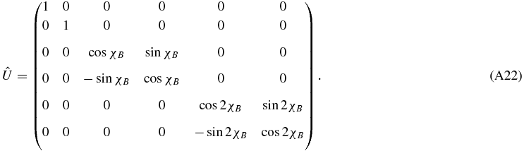
APPENDIX A: THE REDISTRIBUTION MATRICES
In this appendix we give the expression of the Hanle redistribution matrix used in Equation (8) of the text. We use the approximation III of the Hanle redistribution matrix defined in Bommier (1997b) for a two-level atom with unpolarized ground level. In matrix notation, this Hanle redistribution matrix may be written as

RII, III(λ, λ', z) are the angle-averaged redistribution functions of Hummer (1962). Index i (=1, 2, 3, 4, 5) labels different (λ, λ') wavelength domains. We use the same domains as in Bommier (1997b). Indices 1–3 refer to the domains relevant to RIII, and indices 4 and 5 to the domains relevant to RII (see, e.g., Fluri et al. 2003). In Bommier (1997b) the redistribution matrix elements are given in terms of the irreducible spherical tensors. Here we use a matrix notation and work in the irreducible Stokes vector  basis. This implies that we deal with 6 × 6 matrices. For clarity, the explicit expression of the
  matrices are given below.
We introduce the Hanle phase matrix  (see, e.g., Landi Degl'Innocenti & Landolfi 2004), where Γ is the Hanle parameter defined by

Here, gJ is the Landé g factor of the upper level (gJ = 1 for the Ca i 4227 Å line). The magnetic field strength B is expressed in Gauss and ΓR in units of 107 s−1. We also introduce the diagonal matrices


with  being the identity matrix,


and the coefficients

The coefficients α and β(K) are branching ratios introduced in Bommier (1997b, see her Equation (88)). They are given by


with D(0) = 0 and D(2) = cΓE, where c is a constant, taken to be 0.379 (see Faurobert-Scholl 1992).
The expressions given in Bommier (1997b) involve a cutoff frequency vc(a), which is given by the solution of the equation

and a constant  coming from the angle-averaging process. The incident and scattered non-dimensional frequencies are denoted by x' and x. The matrices
  , together with the frequency domains, can be written in the following algorithmic form:
If

then domain 1:

elseif

then domain 2:

else domain 3:

endif.
If

then domain 4:

else domain 5:

endif.
We note that in the CRD approximation we set α = 0, βK = 1 − and RIII(λ, λ', z) = ϕ(λ, z)ϕ(λ', z).
The Hanle phase matrix  is given below:

where
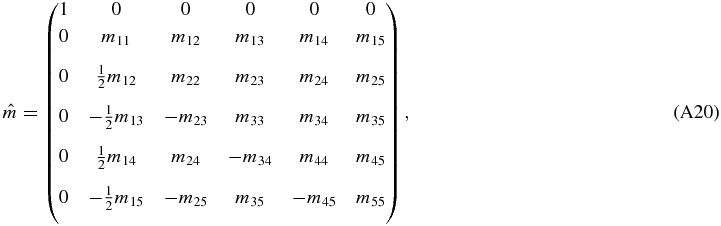
with
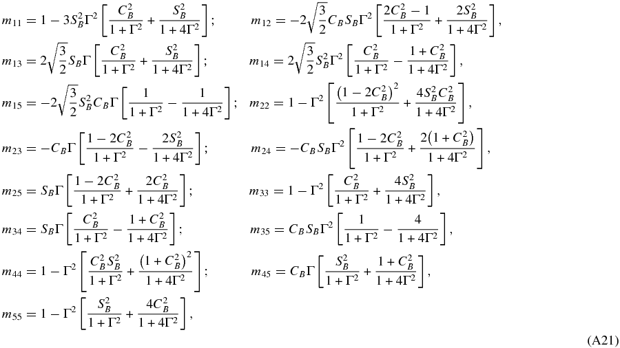
with CB = cos θB, SB = sin θB. The matrix  is given by
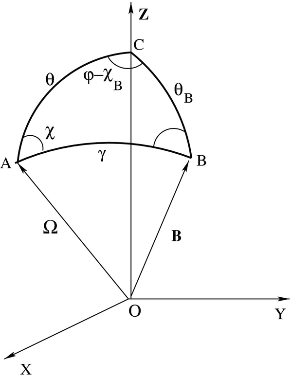
APPENDIX B: THE ZEEMAN RT IN THE ATMOSPHERIC REFERENCE FRAME
The definition of the Zeeman absorption matrix is usually given in an orthogonal reference frame with the z-axis along the LOS. This reference frame is adequate for LTE transfer problems which can be solved ray by ray. Here we must solve the Zeeman transfer equation (Equation (12)) in the atmospheric reference frame (with the z-axis along the atmospheric normal). In the LOS reference frame the elements of the Zeeman absorption matrix depend on the angle γ between the LOS and the direction of the magnetic field vector  , and on χ that represents the azimuth of
  in the transversal plane. In practice the dependence is on cos γ and on cosine and sine of χ and 2χ. Here we show how to express the angular dependence of the Zeeman absorption matrix in terms of the polar angles (θ,φ) of the ray direction
  and (θB,χB) of the vector
  (see Figure 13). We note in Figure 13 that the values of θB, θ, and γ form a spherical triangle, if θ and γ are non-zero. We use spherical trigonometry (see Smart 1960) to transform the terms depending on γ and χ. The geometrical factors entering the Zeeman absorption matrix are cos γ, cos 2γ, sin 2γcos 2χ, and sin 2γsin 2χ. The factor cos γ is simply expressed by the cosine rule

from which we get the factor cos 2γ

Using the sine rule and an analogue of the sine rule we get

and

Subtracting the square of Equation (B3) from the square of Equation (B4) we get

Multiplying Equation (B3) by Equation (B4) and multiplying by a factor of two on both sides of the resulting equation we get

Figure 13. Angles defining the transformation between the line-of-sight reference frame and the atmospheric reference frame, with respect to which both the Zeeman and Hanle line transfer problems are defined in the present paper.
Download figure:
Standard image High-resolution image
Footnotes
- 6
The values of χB are actually defined in a local coordinate system attached to each observation point. Corrections for this effect are not taken into account. They are smaller than 10% as the slab is 184 arcsec for a solar diameter of 1920 arcsec.