


ABSTRACT
We used a large, homogeneous sample of 4178 z ⩽ 0.8 Seyfert 1 galaxies and QSOs selected from the Sloan Digital Sky Survey to investigate the strength of Fe ii emission and its correlation with other emission lines and physical parameters of active galactic nuclei. We find that the strongest correlations of almost all the emission-line intensity ratios and equivalent widths (EWs) are with the Eddington ratio (L/LEdd), rather than with the continuum luminosity at 5100 Å (L5100) or black hole mass (MBH); the only exception is the EW of ultraviolet Fe ii emission, which does not correlate at all with broad-line width, L5100, MBH, or L/LEdd. By contrast, the intensity ratios of both the ultraviolet and optical Fe ii emission to Mg ii λ2800 correlate quite strongly with L/LEdd. Interestingly, among all the emission lines in the near-UV and optical studied in this paper (including Mg ii λ2800, Hβ, and [O iii] λ5007), the EW of narrow optical Fe ii emission has the strongest correlation with L/LEdd. We hypothesize that the variation of the emission-line strength in active galaxies is regulated by L/LEdd because it governs the global distribution of the hydrogen column density of the clouds gravitationally bound in the line-emitting region, as well as its overall gas supply. The systematic dependence on L/LEdd must be corrected when using the Fe ii/Mg ii intensity ratio as a measure of the Fe/Mg abundance ratio to study the history of chemical evolution in QSO environments.
Export citation and abstract BibTeX RIS
1. INTRODUCTION
Fe ii multiplet emission is a prominent feature in the ultraviolet (UV) to optical spectra of most active galactic nuclei (AGNs), including QSOs at redshifts as high as ≳ 6 (e.g., Barth et al. 2003; Freudling et al. 2003; Iwamuro et al. 2004; Jiang et al. 2007; Kurk et al. 2007). Its equivalent width (EW) varies significantly from object to object, ranging from >100 Å to undetectable (<5 Å (1σ)) for the Fe ii λ4570 blend in the 4434–4684 Å region (Boroson & Green 1992). Fe ii emission is an important probe of AGN physics. For example, Boroson & Green (1992) showed that the strength of the Fe ii λ4570 emission relative to [O iii] λ5007 is a dominant variable in the first principal component (PC1 or Eigenvector 1) in their analysis of the correlation matrix of QSO properties, which is generally believed to be linked to certain fundamental parameters of the accretion process (e.g., the relative accretion rate, often expressed as L/LEdd or L/M; Sulentic et al. 2000b; Boroson 2002). Fe ii emission is a strong coolant of the broad-line region (BLR) of AGNs, and thus provides useful information about the BLR from energy budget considerations (Osterbrock & Ferland 2006; see also Vestergaard & Wilkes 2001, and references therein). More importantly, Fe ii emission relative to that of α-elements (e.g., Mg ii) can be considered to be an observational proxy of the Fe/α abundance ratio. If iron is mainly produced by Type Ia supernovae, which have long-lived progenitors, this ratio would have a characteristic delay of ∼1 Gyr from the initial starburst in the QSO host environment. Thus, Fe ii emission in principle can serve as a cosmic clock to constrain the age of QSOs and the epoch of the first star formation in their host galaxies (Hamann & Ferland 1993; and cf., e.g., Matteucci & Recchi 2001).
However, the ionization and excitation mechanisms of the Fe ii emission are very complex due to the low ionization potential of the Fe0 atom (7.9 eV), the low energy levels of the various excited states of Fe+, and particularly the complexity of its atomic structure (see Baldwin et al. 2004; Collin & Joly 2000 and references therein; Joly et al. 2008). Thus, the conversion from Fe ii emission to iron abundance is not straightforward (e.g., Baldwin et al. 2004; Verner et al. 2004). Furthermore, it is possible that Fe ii emission in AGNs arises from several different sites with similarly suitable excitation conditions, including gaseous clouds gravitationally bound in the BLR and narrow-line region (NLR), (the base of) outflows, and the surface of the accretion disk (see, e.g., Collin-Souffrin 1987; Murray & Chiang 1997; Matsuoka et al. 2007; Zhang et al. 2007). This has already been hinted at by the reverberation mapping observations of Fe ii emission, particularly of its optical component, since the cross-correlation function appears to be ill-defined, being broad and flat-topped (Vestergaard & Peterson 2005; Kuehn et al. 2008; see also Kollatschny & Welsh 2001; Wang et al. 2005). Therefore, to use Fe ii emission as a proxy to estimate Fe abundance and to constrain chemical evolution requires a better understanding of its origin and emission mechanisms. In fact, it is well known that the Fe ii/Mg ii intensity ratios of QSOs at the same redshift have a rather large scatter (e.g., Dietrich et al. 2003; Iwamuro et al. 2004; Leighly & Moore 2006).
It is also possible that the excitation mechanisms and sites of Fe ii emission are well governed by certain fundamental parameters (such as Eddington ratio, L/LEdd)8 due to some self-regulation mechanisms that maintain the normal dynamically quasi-steady states of the gas surrounding the central engine of AGNs. Recently, Dong et al. (2009b) found that the EW of the Mg ii λ2800 emission line does not depend intrinsically on AGN luminosity, broad-line width, or BH mass, but is governed solely and strongly by L/LEdd.9 If this is also true for Fe ii emission, then, by accounting for the dependence on L/LEdd, it may be possible to calibrate the relationship between the Fe ii/Mg ii intensity ratio and the Fe/Mg abundance ratio, and thus constrain chemical evolution in QSO environments.
Motivated by these considerations, we carry out a systematic study of the strengths of UV and optical Fe ii emission, by taking advantage of the unprecedented spectroscopic data from the Sloan Digital Sky Survey (SDSS; York et al. 2000). Using the identification and measurement of Fe ii emission lines from Véron-Cetty et al. (2004), we are also able to study narrow-line Fe ii emission systematically for the first time. The paper is organized as follows. In Section 2 we describe the selection criteria of the sample, the spectral fitting and measurements, investigation of Fe ii strength with respect to continuum and other emission lines, and correlation and regression analyses. Section 3 presents the results and our discussion. Section 4 gives conclusions and implications. Throughout this paper, we use a cosmology with H0 = 70 km s−1 Mpc−1, Ωm = 0.3, and ΩΛ = 0.7.
2. DATA ANALYSIS
2.1. Sample and Spectral Fitting
2.1.1. Sample Construction
We first construct a homogenous sample of Seyfert 1s and QSOs (namely type 1 AGNs) from the spectral data set of the SDSS Fourth Data Release (Adelman-McCarthy et al. 2006), according to the following criteria: (1) redshift z ⩽ 0.8; (2) median signal-to-noise ratio (S/N) ⩾10 pixel−1 in the optical Fe ii and Hβ region (4400–5400 Å); (3) weak stellar absorption features, such that the rest-frame EWs of Ca ii K (3934 Å), Ca ii H + H (3970 Å), and Hδ (4102 Å) absorption features are undetected at <2σ significance. The redshift cut is set to ensure that Hβ and the Fe ii λ4570 multiplets are present in the SDSS bandpass. The S/N criterion allows proper placement of local continua and the accurate measurement of emission lines (especially broad and narrow Fe ii emission). The third criterion ensures that the AGN luminosity and emission-line EWs suffer minimally from contamination by host galaxy starlight. Normally, the Ca ii K absorption feature alone can effectively gauge the level of starlight contamination; however, in AGN-dominated spectra, the measurement of this feature in practice can be affected by nearby emission lines in the continuum windows. So, we visually inspect the spectra that have Ca ii K absorption detected at ⩾2σ but no Ca ii H + H or Hδ absorption features detected at ⩾1σ significance. A small fraction (∼10%) of the objects are retained in this way. To quantify the level of galaxy contamination imposed by our selection process, we simulated artificial spectra by combining different proportions of template spectra of pure AGNs (high-luminosity QSOs) and pure starlight (absorption-line or weak star-forming galaxies). As described in greater detail in the Appendix, our selection criterion corresponds to a galaxy contribution of ≲ 10% around 4200 Å. Compared to other sources of errors (see Section 2.1.2), this level of starlight contamination has little effect on the emission-line measurements; it contributes at most 0.002 dex (0.5%) to the variance of emission-line EWs.
After removing duplications and sources with excessive bad pixels in the Hβ or Fe ii λ4570 region, our final sample consists of 4178 type 1 AGNs (hereinafter the full type 1 sample). Of these, 2092 have redshifts z ≳ 0.45 and median S/N ≳ 10 pixel−1 in the UV Fe ii region (2200–3090 Å); this UV subsample will be used to examine the behavior of UV Fe ii and Mg ii λ2800.
2.1.2. Spectral Fitting and Measurements
We use the measured parameters from the Value-added ExtraGAlactic Catalog developed and maintained by the Center for Astrophysics at the University of Science and Technology of China (USTC–VEGAC; X.-B. Dong et al. 2011, in preparation; J.-G. Wang et al. 2011, in preparation). Details of the spectral fitting in the optical and near-UV regions have been described in Dong et al. (2008) and Wang et al. (2009), respectively. Here, we present a brief description of the continuum and emission-line fits. The fits are based on the MPFIT package (Markwardt 2009), which performs χ2-minimization using the Levenberg–Marquardt technique. We corrected the spectra for Galactic extinction using the extinction map of Schlegel et al. (1998) and the reddening curve of Fitzpatrick (1999).
The optical Fe ii is modeled with two separate sets of templates in analytical forms,10 one for the broad-line system and the other for the narrow-line system. These two sets of templates are constructed from measurements of I Zw 1 by Véron-Cetty et al. (2004), as listed in their Tables A1 and A2; see Dong et al. (2008) for details. Within each system, the respective set of Fe ii lines are assumed to have no relative velocity shifts and the same relative strengths as those in I Zw 1. The UV Fe ii is modeled with the tabulated semi-empirical template for I Zw 1 generated by Tsuzuki et al. (2006). In the wavelength region covered by Mg ii emission, they employed a semi-empirical iteration procedure to build the template. They first generated a theoretical Fe ii model spectrum with the photoionization code CLOUDY (Ferland et al. 1998) and subtracted it from the observed spectrum of I Zw 1 around Mg ii. Then the Mg ii doublet lines were fit assuming each line has the same profile as Hα, and finally they obtained the Fe ii template underneath Mg ii by subtracting the Mg ii fit from the observed spectrum. The separation of narrow and broad lines was not taken into account for the UV Fe ii template, but narrow lines in the UV are generally weak (e.g., Laor et al. 1994).
Each line in the Mg ii doublet is fitted with a truncated five-parameter Gauss–Hermite series (Wang et al. 2009; see also Salviander et al. 2007). As the profile of broad Hβ is sometimes rather complex, it is fitted with as many Gaussians as statistically justified; we do not ascribe any particular physical significance to the individual Gaussian components (Dong et al. 2005). We assume that the broad Fe ii lines have the same profile as broad Hβ (see Boroson & Green 1992; Landt et al. 2008; cf. Hu et al. 2008b), but we leave their relative velocity as a free parameter. The fluxes of both broad and narrow Fe ii emission are quite insensitive to the exact line width (Vestergaard & Peterson 2005; Landt et al. 2008) and profile shape assumed for the broad component, which is verified at the end of this section. All narrow emission lines are fitted with a single Gaussian, except for the [O iii] λλ4959, 5007 doublet lines, each of which is modeled with two Gaussians, one accounting for the line core and the other for a possible blue wing seen in many objects. The redshift and width of narrow-line Fe ii are set as free parameters.
The presence of optical narrow Fe ii emission lines in AGNs has been long overlooked. Previously, narrow Fe ii emission has been studied in only a few objects (in the near-UV: Vestergaard & Wilkes 2001; Wang et al. 2008; in the optical: Véron-Cetty et al. 2004, 2007; Bruhweiler & Verner 2008; cf. Section 4.6 of Hu et al. 2008b). A companion paper (Dong et al. 2010), drawn directly from the current sample and analysis, presents the first systematic study of the prevalence of optical narrow Fe ii emission lines in type 1 AGNs and their non-detection in type 2 AGNs. Whether there is a physically distinct boundary between the NLR and BLR is still debated (cf. Laor 2007), particularly considering the likely presence of a region intermediate between them (e.g., the intermediate-line region, Brotherton et al. 1994; the inner NLR, Nagao et al. 2003; see Zhang et al. 2009 for a concise review), and the fact that both the BLR and NLR may be highly stratified and multi-zoned. In this paper, we follow Véron-Cetty et al. (2004), who divided the Fe ii spectrum phenomenologically into two main kinematic sub-systems: a broad (L1; FWHM ≈1100 km s−1) component associated with other prominent broad emission lines, and a narrow (N3; FWHM ≈280 km s−1) component, consisting of both permitted and forbidden transitions, associated with other low-excitation narrow lines. In I Zw 1, there are two additional narrow-line systems, N1 and N2, that appear only in high-excitation lines (not in Fe ii); N1 and N2 are relatively broad and blueshifted (by 1450 and 500 km s−1, respectively), whereas N3 is almost at the systemic redshift of the host galaxy. The broad-line system L1 is also blueshifted by 150–200 km s−1 in both the optical and UV bands (Laor et al. 1997; Véron-Cetty et al. 2004), which distinguishes it from the narrow-line system N3 and made possible the unambiguous identification of narrow Fe ii lines (P. Véron 2009, private communication).
Figure 1 shows the optical spectrum and spectral decomposition of a representative object in our sample (SDSS J092801.30+491817.3). In this object, the optical Fe ii lines have a width (corrected for the instrumental broadening of FWHM = 130 km s−1) of FWHM = 1300 km s−1 for the broad component and FWHM = 250 km s−1 for the narrow component. Note that the individual narrow Fe ii lines marked in the figure (particularly the forbidden lines) are sharp and distinct from nearby broad Fe ii lines, which indicates that our identification and decomposition of the narrow component is robust, not residuals from poor broad Fe ii subtraction due to mismatch of the broad Fe ii model. Strong narrow Fe ii emission is found in AGNs of diverse types: broad-line and narrow-line Seyfert 1s, QSOs with and without broad absorption lines, and radio-loud and radio-quiet systems. Figure 2 displays a sample of spectra in which strong narrow Fe ii emission is seen; the object shown in the bottom panel is the low-ionization broad absorption-line QSO FBQS J152350.4+391405, which is a powerful (L5 GHz = 4.0 × 1031 erg s−1 Hz−1), variable radio source (Becker et al. 2000). An example of spectral fitting for the UV subsample is shown in Figure 3. The detailed decompositions of the line profiles of Hβ and Mg ii have been demonstrated in Dong et al. (2008; their Figure 2) and Wang et al. (2009; their Figure 1), respectively.
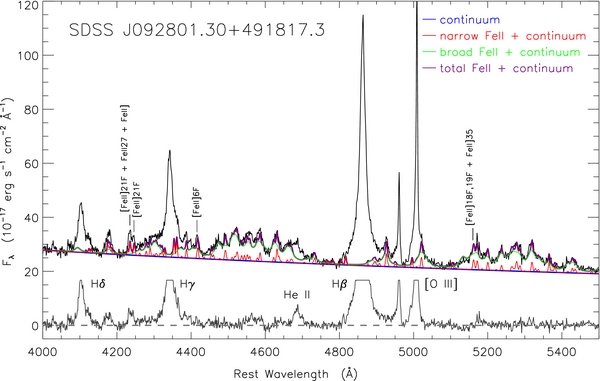
Figure 1. Demonstration of spectral fitting in the optical region. We show the SDSS spectrum (black), the local AGN continuum (blue), the continuum plus narrow-line Fe ii emission (red), the continuum plus broad-line Fe ii emission (green), the pseudocontinuum (continuum plus total Fe ii, purple), and the pseudocontinuum-subtracted residuals (gray). Also marked are some narrow Fe ii lines (particularly the forbidden lines) that are sharp and distinct from nearby broad Fe ii lines. The strong emission lines in the residual spectrum are truncated for clarity.
Download figure:
Standard image High-resolution image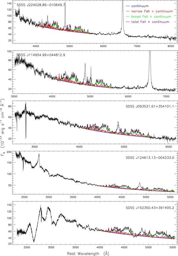
Figure 2. Examples of SDSS spectra of different classes of AGNs with strong narrow Fe ii emission. Also plotted is our continuum fitting in the rest-frame wavelength range 4000–5600 Å. Individual spectral components are denoted as in Figure 1.
Download figure:
Standard image High-resolution image
Figure 3. Demonstration of the continuum fitting in the UV region. We show the SDSS spectrum (black), the local AGN continuum (blue), the pseudocontinuum (continuum plus Fe ii emission, purple), and the pseudocontinuum-subtracted residuals (gray).
Download figure:
Standard image High-resolution imageThe emission-line fluxes are measured from the best-fit models of the line profiles. The EWs are calculated in the rest frame from the best-fit models of both the emission lines and their underlying local continuum, by integrating the line profile with respect to the continuum level pixel by pixel. The fluxes and EWs of narrow and broad optical Fe ii λ4570 emission are integrated in the wavelength range 4434–4684 Å, and those for UV Fe ii are integrated in the range 2200–3090 Å. For all measured emission-line fluxes and EWs, we regard the values as reliable detections when they have greater than 2σ significance; otherwise, we adopt the value plus the 2σ error as an upper limit (see Section 2.1.3 for the estimation of measurement errors). Using 2σ significance instead of the more commonly used 3σ one is a trade-off we have made in order to obtain a sample sufficiently large to explore parameter space, particularly for narrow Fe ii (see Figure 11). We have verified that none of our main conclusions are affected by this particular choice. The continuum and emission-line parameters for the optical and UV subsamples are listed in Tables 1 and 2, respectively; we make available online all the detailed fitting results.11
Table 1. Optical Continuum and Emission-line Parameters of the Full Sample
| SDSS Name | z | log L5100 | β | FWHM(HβB) | log F(Fe iiN) | EW(Fe iiN) | log F(Fe iiB) | EW(Fe iiB) | log F(HβN) | log F(HβB) | EW(HβB) | log F([O iii] λ5007) | EW([O iii] λ5007) |
|---|---|---|---|---|---|---|---|---|---|---|---|---|---|
| (1) | (2) | (3) | (4) | (5) | (6) | (7) | (8) | (9) | (10) | (11) | (12) | (13) | (14) |
| J000011.96+000225.2 | 0.4790 | 44.69 | −2.45 | 3034 | −14.96 | 7.6 | −13.99 | 71.5 | −15.68 | −13.89 | 104.9 | −14.87 | 11.7 |
| J000043.95−091134.9 | 0.4388 | 44.62 | −1.59 | 5973 | < −16.16 | <0.5 | −14.34 | 33.4 | −16.00 | −14.29 | 41.1 | −15.02 | 8.1 |
| J000102.19−102326.8 | 0.2943 | 44.20 | −1.00 | 7748 | −16.04 | 0.7 | −14.98 | 8.2 | −15.16 | −14.02 | 81.3 | −14.20 | 55.4 |
| J000109.14−004121.5 | 0.4166 | 44.32 | −1.62 | 1899 | −16.09 | 1.0 | −14.67 | 27.2 | −15.52 | −14.60 | 35.1 | −14.99 | 15.0 |
| J000110.96−105247.4 | 0.5283 | 44.98 | −2.23 | 6806 | < −16.13 | <0.3 | −14.11 | 35.3 | −15.53 | −13.73 | 97.2 | −14.52 | 16.8 |
| J000111.21−002011.2 | 0.5178 | 44.51 | −1.63 | 3465 | −15.55 | 3.8 | −14.47 | 46.3 | −15.80 | −14.14 | 110.1 | −14.54 | 46.2 |
| J000115.99+141123.0 | 0.4037 | 44.38 | −1.37 | 5178 | < −16.15 | <0.7 | −14.98 | 11.2 | −16.42 | −14.13 | 85.6 | −14.36 | 53.0 |
Notes. Column 1: official SDSS name; Column 2: redshift measured by the SDSS pipeline; Column 3: luminosity of the power-law continuum at 5100 Å, λLλ(5100 Å); Column 4: local continuum slope fitted in the rest-frame wavelength range of 4000–5600 Å (fλ = λβ); Column 5: FWHM of broad Hβ, corrected for instrumental broadening; Column 6: flux of narrow Fe ii λ4570 (integrated in the range of 4434–4684 Å from the best-fit model); Column 7: rest-frame EW of narrow Fe ii λ4570; Column 8: flux of broad Fe ii λ4570 (integrated in the range of 4434–4684 Å from the best-fit model); Column 9: rest-frame EW of broad Fe ii λ4570; Column 10: flux of the narrow component of Hβ; Column 11: flux of the broad component of Hβ; Column 12: rest-frame EW of the broad component of Hβ; Column13: flux of [O iii] λ5007; Column14: rest-frame EW of [O iii] λ5007. Luminosities, fluxes, EWs, and FWHM are in units of erg s−1, erg s−1 cm−2, Å, and km s−1, respectively.
Only a portion of this table is shown here to demonstrate its form and content. A machine-readable version of the full table is available.
Download table as: DataTypeset image
Table 2. Near-UV Continuum and Emission-line Parameters of the UV Subsample
| SDSS Name | log L3000 | FWHM(Mg iiB) | log F(UV Fe ii) | EW(UV Fe ii) | log F(Mg iiN) | log F(Mg iiB) | EW(Mg iiB) |
|---|---|---|---|---|---|---|---|
| (1) | (2) | (3) | (4) | (5) | (6) | (7) | (8) |
| J000011.96+000225.2 | 45.02 | 2898 | −13.04 | 180.6 | −15.81 | −13.79 | 35.4 |
| J000110.96−105247.4 | 45.24 | 6135 | −13.33 | 77.3 | −15.06 | −13.90 | 22.4 |
| J000111.21−002011.2 | 44.71 | 2601 | −13.77 | 93.3 | −15.44 | −14.46 | 20.1 |
| J000559.20+153125.1 | 44.65 | 3014 | −13.38 | 179.5 | −15.88 | −13.98 | 50.2 |
| J000945.46+001337.1 | 45.12 | 2342 | −13.46 | 149.3 | −15.99 | −14.32 | 22.0 |
| J001024.22+153331.3 | 45.69 | 3317 | −13.08 | 102.0 | −15.72 | −13.92 | 15.9 |
| J001104.84−092357.8 | 45.08 | 2199 | −13.57 | 126.5 | −16.07 | −14.45 | 17.6 |
Notes. Column 1: official SDSS name; Column 2: luminosity of the power-law continuum at 3000 Å, λLλ(3000 Å); Column 3: FWHM of broad Mg ii λ2800, corrected for instrumental broadening; Column 4: flux of near-UV Fe ii emission (integrated in the range of 2200–3090 Å from the best-fit model); Column 5: rest-frame EW of UV Fe ii emission; Column 6: flux of the narrow component of Mg ii λ2800; Column 7: flux of the broad component of Mg ii λ2800; Column 8: rest-frame EW of the broad component of Mg ii λ2800. Luminosities, fluxes, EWs, and FWHM are in units of erg s−1, erg s−1 cm−2, Å, and km s−1, respectively.
Only a portion of this table is shown here to demonstrate its form and content. A machine-readable version of the full table is available.
Download table as: DataTypeset image
Lastly, to test the effect of our adopted broad Fe ii line profile on the flux measurements of both broad and narrow Fe ii emission, we experimented with an alternative scheme in which a single Lorentzian with adjustable width is used to model the profile of the individual broad Fe ii lines. This choice is inspired by the fact that the broad Fe ii lines in I Zw 1 are well described by a Lorentzian profile (Véron-Cetty et al. 2004). This alternate scheme yields broad Fe ii line widths that are on average only 0.3 times the broad Hβ with a standard deviation of 0.2 dex (46%), but the line fluxes—the main focus of this study—are statistically unchanged. We find that the fluxes of broad  emission (hereinafter
  ) are similar to those of our default scheme within 0.3 dex (70%) for 97% (4055/4178) of the sample, while the fluxes of narrow
  (hereinafter
  ), agree to within 0.3 dex for 88% of the objects. This is illustrated in Figure 4, where, for clarity, we only plot the objects with fluxes detected at >3σ significance by both schemes. As already reported in Vestergaard & Peterson (2005, their Section 2.3.4) and Landt et al. (2008, their Section 4.4), the broad Fe ii multiplets are so highly blended that their summed overall profile mainly depends on the relative strengths of the multiplets rather than on their velocity widths. According to their experiments, changing the width of the broad Fe ii template (constructed from I Zw 1, which has FWHM = 1100 km s−1) by as much as several thousand km s−1 has only a minor effect on the resulting line fluxes, especially for the cases with larger line widths. Thus, we are confident that the fluxes of both the broad and narrow Fe ii emission, integrated over a large wavelength range, are very insensitive to the exact profile shape or width assumed for the individual broad lines.

Figure 4. Fluxes of broad (left) and narrow (right) Fe ii λ4570 emission detected at >3σ significance, calculated from the best fits using two different schemes: the default scheme where the profile of broad Fe ii is set to that of broad Hβ, and another where broad Fe ii is modeled as a Lorentzian with variable width. The 1σ relative errors for the fluxes of broad and narrow Fe ii λ4570 are only 11% and 17%, respectively. These errors are estimated from the bootstrap method and do not account for the uncertainties caused by possible Fe ii template mismatch.
Download figure:
Standard image High-resolution image2.1.3. Estimation of Parameter Uncertainties
The errors on the fitted parameters provided by MPFIT only account for formal statistical uncertainties and likely underestimate the true uncertainties. They do not include potential systematic uncertainties introduced by, for example, line deblending or pseudocontinuum subtraction (see Marziani et al. 2003 for a detailed discussion).
We estimate the measurement uncertainties due to line deblending using a bootstrap method (Dong et al. 2008; Wang et al. 2009), as follows. We generate 500 spectra by randomly combining the scaled, model emission lines of one object (denoted as "A") to the emission line-subtracted spectrum of another object (denoted as "B"). In order to minimize changes in S/N within the emission-line spectral regions in the simulated spectra, the emission-line model of object "A" is scaled in such a way that it has the same flux for the line in question as in object "B." Then, we fit the simulated spectra following the same procedure as described in Section 2.1.2. For each parameter, we consider the error typical of our sample to be the standard deviation of the relative difference between the input and the recovered parameter values. These relative differences turn out to be normally distributed for each of the parameters concerned. The estimated typical 1σ relative errors are 0.043 dex (10%), 0.035 dex (8%), 0.043 dex (10%), 0.052 dex (12%), 0.048 dex (11%), and 0.074 dex (17%), respectively, for the fluxes of broad Mg ii, broad Hβ, [O iii] λ5007, UV Fe ii, broad Fe ii λ4570, and narrow Fe ii λ4570; 0.087 dex (20%) and 0.065 dex (15%), respectively, for the FWHM of broad Mg ii and Hβ; and 0.035 dex (8%) and 0.022 dex (5%), respectively, for the slope and normalization of the local continua. The errors on EWs are calculated using standard propagation of errors. In the analysis of Sections 2.2 and 2.3, we generally adopt the errors based on the bootstrap method, with the exception of a minority of objects in which the bootstrap errors are actually smaller than the formal MPFIT errors, in which case we adopt the latter.
The uncertainties due to pseudocontinuum subtraction are harder to estimate. Two factors come into play. The first is due to the choice of Fe ii template. Although we have adopted the latest improvements to the Fe ii template (Véron-Cetty et al. 2004; Tsuzuki et al. 2006), the fact remains that essentially all templates used in this field, including ours, are derived ultimately from observations of a single AGN, namely I Zw 1. Our choice of using these templates is motivated entirely by pragmatism: empirically, they seem to work, and they are the best we have at the moment. Unfortunately, there is currently no practical way to quantify the uncertainties that might be introduced by this restriction.
For a given choice of Fe ii template, additional uncertainties arise from the fitting procedure, since we must assume a profile for the broad Fe ii lines, which are too highly blended to be determined independently. Our default fitting scheme—motivated by previous studies—assumes that the broad components of Fe ii and Hβ have exactly the same profile. In detail, of course, this cannot be strictly true. To estimate the likely impact of this assumption, we refit the spectra assuming that Fe ii has a Lorentzian profile (Section 2.1.2 and Figure 4). The standard deviations of the differences in flux between our default scheme and the Lorentzian scheme are 0.09 dex (21%) and 0.12 dex (28%) for broad and narrow Fe ii λ4570, respectively. We suspect that uncertainties of roughly this magnitude (∼0.1 dex) can potentially affect the fluxes of all the Fe ii lines, as well as those of Mg ii and [O iii], which are strongly affected by Fe ii contamination. This additional uncertainty was added to the error budget of the fluxes of these lines. We do not consider this error contribution to the fluxes of other narrow lines or of broad Hβ, the bulk of which is not severely affected by Fe ii emission.
The continuum luminosities employed in our analysis are affected not only by Fe ii subtraction, but also, to some degree, by host galaxy contamination, despite our efforts to mitigate it (see the Appendix). The 3000 Å continuum is additionally influenced by our treatment of the Balmer continuum (Wang et al. 2009). Taking all of these factors into consideration, we estimate that the continuum luminosities at 3000 Å and 5000 Å incur an uncertainty of ∼0.05 dex (12%) on top of that derived from the bootstrapping method.
Typical error bars, which represent the quadrature sum of the uncertainties described above, for the parameters used in our analysis are shown in Figures 5–12. However, because these estimates are only approximate, and it is nearly impossible to derive rigorous errors for every individual object, we will adopt only the bootstrapping errors in the regression analysis below. We will not attempt to estimate the intrinsic scatter of the relations presented in this paper.
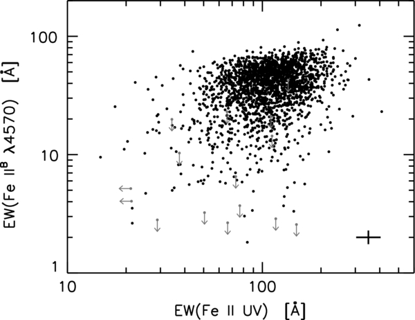
Figure 5. Distribution of EWs of broad Fe ii λ4570 and UV Fe ii emission. Black dots denote reliable detections at ⩾2σ significance; gray arrows give upper limits (see Section 2.1.2). The bottom-right corner shows a representative error bar, the length of which corresponds to the 1σ total error, which includes contributions from uncertainties arising from line deblending and Fe ii fitting (see Section 2.1.3).
Download figure:
Standard image High-resolution image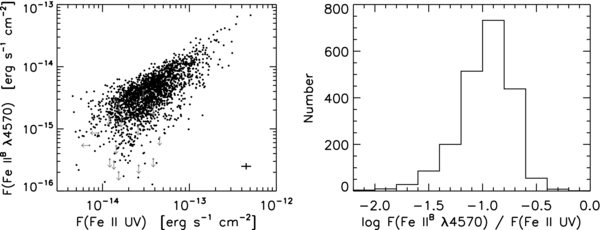
Figure 6. Left: distribution of fluxes of broad Fe ii λ4570 and UV Fe ii emission. The symbols are the same as in Figure 5. Right: histogram of the flux ratios of broad Fe ii λ4570 to UV Fe ii emission, for the objects with both emission lines detected at ⩾2σ significance.
Download figure:
Standard image High-resolution image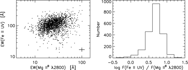
Figure 7. Left: distribution of EWs of UV Fe ii and broad Mg ii λ2800. The symbols are the same as in Figure 5. Right: histogram of the flux ratios of UV Fe ii to broad Mg ii λ2800, for the objects with both emission lines detected at ⩾2σ significance.
Download figure:
Standard image High-resolution image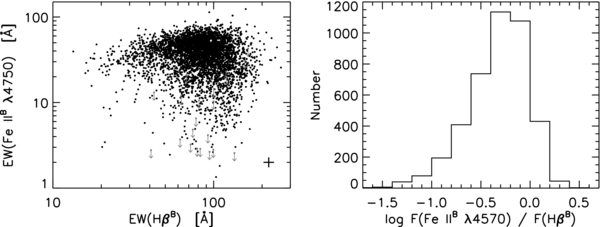
Figure 8. Left: distribution of EWs of broad Fe ii λ4570 and broad Hβ. The symbols are the same as in Figure 5. Right: histogram of the flux ratios of broad Fe ii λ4570 to broad Hβ, for the objects with both emission lines detected at ⩾2σ significance.
Download figure:
Standard image High-resolution image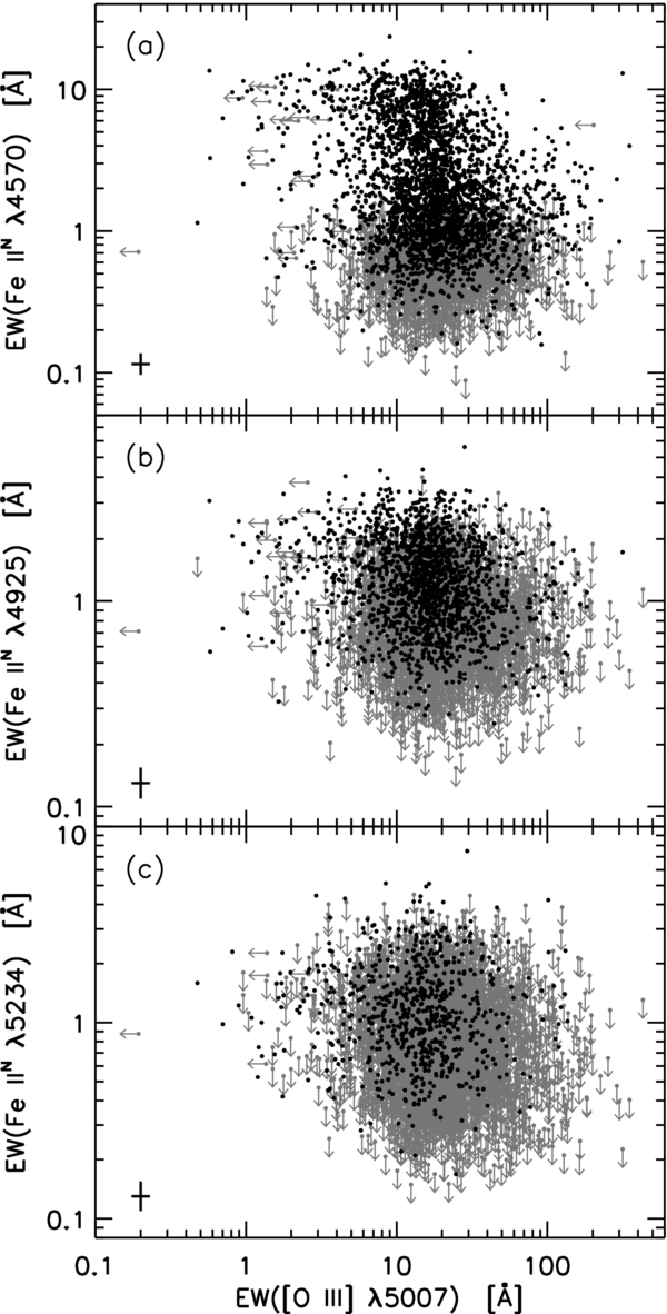
Figure 9. Distribution of EWs of narrow (a) Fe ii λ4570, (b) Fe ii λ4925, and (c) Fe ii λ5234 vs. that of [O iii] λ5007. Fe ii λ4570 and [O iii] λ5007 are measured from the best-fit model, while Fe ii λ4925 and Fe ii λ5234 are measured from the residual spectra after the continuum, broad Fe ii, and other broad emission lines are subtracted. The symbols are the same as in Figure 5.
Download figure:
Standard image High-resolution image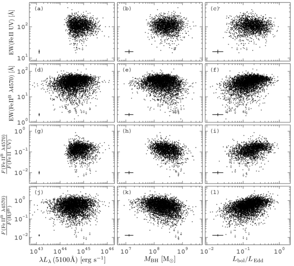
Figure 10. Dependence of broad Fe ii emission on continuum luminosity λLλ(5100 Å), BH mass (MBH), and Eddington ratio (Lbol/LEdd). The symbols are the same as in Figure 5.
Download figure:
Standard image High-resolution image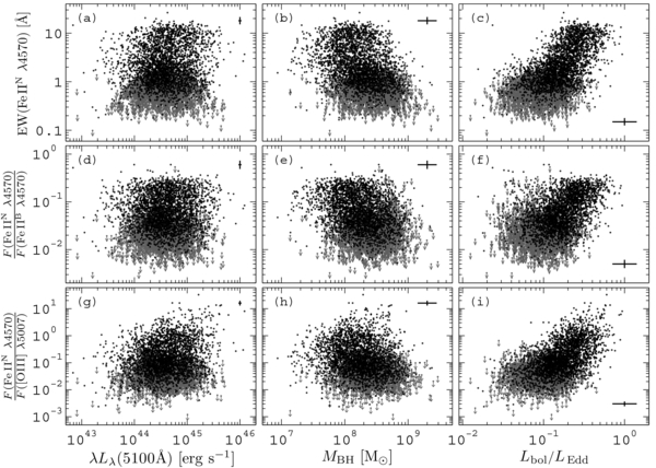
Figure 11. Dependence of narrow Fe ii emission on continuum luminosity λLλ(5100 Å), BH mass (MBH), and Eddington ratio (Lbol/LEdd). The symbols are the same as in Figure 5.
Download figure:
Standard image High-resolution image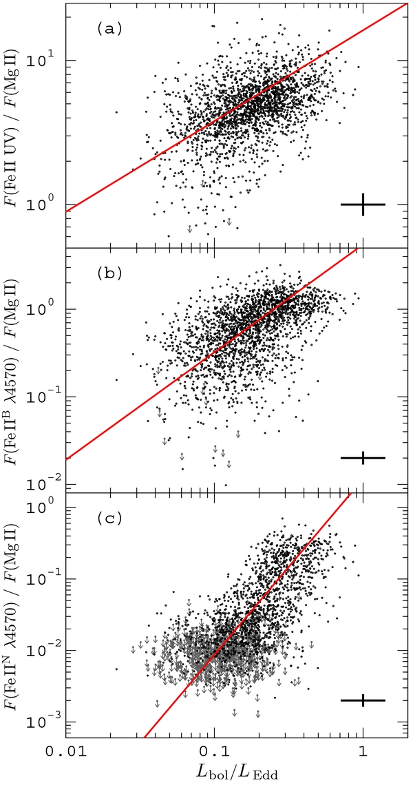
Figure 12. Strength of broad (UV and optical) and narrow Fe ii emission relative to broad Mg ii λ2800 as a function of Eddington ratio. Also plotted are the best-fitting linear relations in log–log scale (see Equations (1)–(3)). The symbols are the same as in Figure 5.
Download figure:
Standard image High-resolution image2.2. The Strength of Fe ii Emission
We calculate the fluxes and rest-frame EWs of strong emission lines and investigate the distributions of the EWs of various Fe ii emissions and their relative strengths with respect to other lines. We have already presented in Dong et al. (2010, their Figure 3) the distributions of the EWs of  and
and  ; the two quantities do not correlate very strongly12 (Spearman coefficient
  , hereinafter in this subsection accounting for upper limits; see Section 2.1.2 for the definition of upper limits), suggesting that the narrow component is not an artifact of measurement uncertainty associated with the deblending of the broad component. The intensity ratios of narrow to broad Fe ii λ4570, for the 2502 objects in which both components are detected at >3σ significance (see Dong et al. 2010), vary by two orders of magnitude, ranging from ∼0.005 to 0.5, with a mean of −1.15 dex (0.07; computed in log-scale, hereinafter for the quantities in this subsection) and a standard deviation of 0.30 dex (circa 0.05 in linear scale equivalently). The distribution of the EWs of
  and UV Fe ii emission is displayed in Figure 5 for the 2092 objects in the UV subsample. From the EW–EW distribution, the Fe ii emissions in the two bands do not appear to be strongly correlated (
 ). Yet, this comparison might be complicated by variations in the continuum shape, since the underlying continuum of the two bands used for the EW calculation spans across a considerable wavelength range. In Figure 6 (left panel), we plot instead the distribution of the fluxes of the two emission blends, which now show a fairly strong correlation (
 ). This is also reflected in the histogram of their flux ratios (right panel), for 2076 of the 2092 objects wherein both blends are reliably detected (at ⩾2σ significance, see Section 2.1.2), which clusters around a mean of −0.96 dex (0.11) with a standard deviation of only 0.25 dex (0.06; see also Sameshima et al. 2011). A similar result holds for the relationship between UV Fe ii and Mg ii (
 ; Figure 7);13 the ratios of UV Fe ii to Mg ii flux peak at 0.67 dex (4.70) with a standard deviation of 0.21 dex (2.27).
  and broad Hβ are less strongly correlated (
 ; Figure 8); their flux ratios have a mean of −0.33 dex (0.47) and a standard deviation of 0.30 dex (0.32). The strength of
  does not correlate at all with that of [O iii] λ5007 (Spearman chance probability Pnull = 0.2 for their flux–flux relationship; see also Figure 9(a) for their EW–EW distribution). In order to check if the measurement of narrow Fe ii is biased by the narrow Fe ii template we used, we further calculate the EWs of two other narrow Fe ii features directly from the residual spectra (after the continuum, broad Fe ii, and other emission lines, except narrow Fe ii, are subtracted), namely Fe ii λ4925 (integrated over the vacuum wavelength range 4918–4938 Å, which is dominated by Fe ii 42 λ4923 and Fe ii] λ4928) and Fe ii 49 λ5234. These two features are relatively distinct from nearby broad Fe ii features. The distributions of their EWs are also displayed in Figure 9 (panels b and c); they also do not show any strong correlation with [O iii] at all.
2.3. Correlation and Regression Analysis
We investigate the correlations of the EWs and intensity ratios of narrow and broad Fe ii, broad Mg ii and Hβ, and [O iii] λ5007 with broad-line FWHM, continuum luminosity L5100 ≡ λLλ(5100 Å), MBH, and L/LEdd. We calculate the black hole (BH) masses based on Hβ using the formalism presented in Wang et al. (2009, their Equation (11)). This formalism was calibrated with recently updated reverberation mapping-based masses and assuming that the BLR radius scales with luminosity as R∝L0.5 (Bentz et al. 2009). The Eddington ratios are estimated assuming a bolometric luminosity correction Lbol ≈ 9 λLλ(5100 Å) (Elvis et al. 1994; Kaspi et al. 2000). The mean and standard deviation (computed in log-scale) of the key variables of the sample are as follows: FWHM of broad Hβ, 3.56 dex (3600 km s−1) and 0.22 dex (circa 1820 km s−1 in linear scale equivalently); λLλ(5100 Å), 44.60 dex (4.0 × 1044 erg s−1) and 0.40 dex (3.7 × 1044 erg s−1); MBH, 8.30 dex (2.0 × 108 M☉) and 0.35 dex (1.6 × 108 M☉); L/LEdd, −0.85 dex (0.14) and 0.28 dex (0.09). We assume the 1σ measurement errors for MBH and L/LEdd to be 0.3 dex (70%; Wang et al. 2009).
We perform the bivariate correlation tests using the generalized Spearman rank method implemented in the ASURV package (Isobe et al. 1986). This method tests for not only a linear relation but a monotonic one, and it can handle censored data in both independent and dependent variables. The correlation results are summarized in Table 3, where we report the Spearman coefficient ( ) and the probability (Pnull) that a correlation is not present. Several striking features emerge from the correlation analysis.
- 1.The strongest correlations for the EWs and intensity ratios of all emission lines are with either L/LEdd or broad-line FWHM. For a particular emission-line EW or intensity ratio, the correlations with FWHM and with L/LEdd are almost equally strong, and both are much stronger than those with MBH or L. The correlation with L is generally the weakest.
- 2.The EW of UV Fe ii has no significant correlation with L/LEdd (Pnull = 0.04), or with the other three quantities, but the EWs of optical Fe ii, both broad and narrow, show moderate to strong, positive correlations with L/LEdd (
 for narrow Fe ii and = 0.40 for broad Fe ii, both with Pnull ≪ 10−15).
 - 3.The intensity ratios of Fe ii—both narrow and broad, both in the UV and in the optical—to Mg ii λ2800 correlate strongly and positively with L/LEdd. Among these, the strongest correlation arises from the narrow component of Fe ii ( = 0.70). Interestingly, the intensity ratios of optical Fe ii (narrow and broad) to Mg ii correlate more strongly with L/LEdd than do the EWs of these lines.


Table 3. Results of Spearman Correlation Analysisa
| FWHM (HβB) | L5100b | MBHb | L/LEddb | |
|---|---|---|---|---|
| EW(Fe iiN λ4570) | −0.659(<1e-15) | 0.102(<1e-15) | −0.401(<1e-15) | 0.671(<1e-15) |
| (Fe iiN λ4570)/Mg ii | −0.731(<1e-15) | 0.097(8e-06) | −0.521(<1e-15) | 0.695(<1e-15) |
| (Fe iiN λ4570)/HβB | −0.680(<1e-15) | 0.079(2e-06) | −0.417(<1e-15) | 0.668(<1e-15) |
| (Fe iiN λ4570)/[O iii] λ5007 | −0.606(<1e-15) | 0.140(<1e-15) | −0.319(<1e-15) | 0.626(<1e-15) |
| EW(Fe iiB λ4570) | −0.333(<1e-15) | 0.156(<1e-15) | −0.150(<1e-15) | 0.398(<1e-15) |
| (Fe iiB λ4570)/Mg ii | −0.567(<1e-15) | 0.116(<1e-15) | −0.397(<1e-15) | 0.557(<1e-15) |
| (Fe iiB λ4570)/HβB | −0.474(<1e-15) | 0.064(2e-05) | −0.288(<1e-15) | 0.451(<1e-15) |
| (Fe iiB λ4570)/[O iii] λ5007 | −0.244(<1e-15) | 0.174(<1e-15) | −0.069(8e-06) | 0.336(<1e-15) |
| EW(Fe ii UV) | 0.020(4e-01) | −0.036(7e-02) | −0.018(4e-01) | −0.044(4e-02) |
| (Fe ii UV)/Mg ii | −0.434(<1e-15) | 0.157(<1e-15) | −0.266(<1e-15) | 0.460(<1e-15) |
| (Fe ii UV)/HβB | −0.161(<1e-15) | 0.042(5e-02) | −0.112(<1e-15) | 0.158(<1e-15) |
| (Fe ii UV)/[O iii] λ5007 | −0.068(2e-03) | 0.133(<1e-15) | −0.024(3e-01) | 0.136(<1e-15) |
| (Fe iiN λ4570)/(Fe ii UV) | −0.698(<1e-15) | 0.060(6e-03) | −0.508(<1e-15) | 0.647(<1e-15) |
| (Fe iiB λ4570)/(Fe ii UV) | −0.434(<1e-15) | 0.042(5e-02) | −0.322(<1e-15) | 0.401(<1e-15) |
| (Fe iiN λ4570)/(Fe iiB λ4570) | −0.580(<1e-15) | 0.065(2e-05) | −0.364(<1e-15) | 0.585(<1e-15) |
| EW([O iii] λ5007) | 0.085(4e-08) | −0.128(<1e-15) | −0.029(6e-02) | −0.175(<1e-15) |
| EW(HβB) | 0.333(<1e-15) | 0.110(1e-12) | 0.278(<1e-15) | −0.205(<1e-15) |
| EW(Mg ii) | 0.496(<1e-15) | −0.216(<1e-15) | 0.280(<1e-15) | −0.552(<1e-15) |
Notes.
aFor each entry, we list the Spearman rank correlation coefficient ( ) and the probability of the null hypothesis that the correlation is not present (Pnull) in parenthesis. For the correlations concerning UV emission lines, the data for the 2092 objects in the UV subsample are used; otherwise, those for the 4178 objects in the full sample are used.
bL5100 ≡ λLλ(5100 Å); the BH masses are calculated using the formalism presented in Wang et al. (2009, their Equation (11)); Eddington ratios (L/LEdd) are calculated assuming that the bolometric luminosity Lbol ≈ 9 L5100.
) and the probability of the null hypothesis that the correlation is not present (Pnull) in parenthesis. For the correlations concerning UV emission lines, the data for the 2092 objects in the UV subsample are used; otherwise, those for the 4178 objects in the full sample are used.
bL5100 ≡ λLλ(5100 Å); the BH masses are calculated using the formalism presented in Wang et al. (2009, their Equation (11)); Eddington ratios (L/LEdd) are calculated assuming that the bolometric luminosity Lbol ≈ 9 L5100.
Download table as: ASCIITypeset image
We must note that because the SDSS spectroscopic survey is magnitude-limited, broad-line FWHM, L5100, MBH, and L/LEdd show apparent correlations with one another. The apparent (likely not intrinsic) correlation between MBH and L/LEdd is further enhanced by the correlation of their measurement uncertainties, because both MBH and L/LEdd are constructed from Hβ FWHM and L5100. The Spearman correlation coefficients of L/LEdd with Hβ FWHM, L5100, and MBH are  = −0.70, 0.52, and −0.19, respectively, for the full sample; for the UV subsample, they are
  = −0.82, 0.48, and −0.40, respectively. In light of the serious interdependence among these four quantities, the correlations of emission-line EWs and intensity ratios with L5100 and MBH are probably only a secondary effect of the stronger (thus presumably intrinsic) correlation with L/LEdd (or broad-line FWHM). To test this possibility, we perform a partial correlation analysis using the generalized partial Spearman rank method (Kendall & Stuart 1979; Macklin 1982). The partial correlation results are summarized in Table 4. Because of the strong interdependence among the four physical variables, unfortunately, even partial correlation tests cannot definitively discriminate which variable is the primary driver. However, several trends do stand out clearly.
- 1.First, for all the EWs and intensity ratios that still have significant correlations with MBH or L5100 controlling for L/LEdd (Pnull ≲ 10−3), their correlations with L/LEdd controlling for MBH or L5100 are also significant (Pnull ≪ 10−15). This is just as expected in light of the bivariate correlations, which are weaker with MBH and much weaker with L5100 than with L/LEdd.
- 2.Second, for almost all the EWs and intensity ratios (except the EW of broad Hβ and the ratio of broad Fe ii λ4570 to UV Fe ii) that have significant correlations with FWHM controlling for L/LEdd (Pnull < 10−3), their correlations with L/LEdd controlling for FWHM are also significant (Pnull ⩽ 10−10).
- 3.Third and most important, for some key emission-line quantities, namely the EWs of broad Fe ii λ4570, Mg ii λ2800, and [O iii] λ5007, the ratio of broad Fe ii λ4570 to [O iii] λ5007 (the dominating variable of the PC1 of Boroson & Green 1992), and the ratio of UV Fe ii to Mg ii λ2800 (the common proxy for abundance ratio Fe/α), their correlations are very significant with L/LEdd controlling for L5100, MBH, or FWHM (Pnull ≪ 10−15), but are much less significant (or not significant at all) with L5100, MBH, and even FWHM controlling for L/LEdd (Pnull > 10−8 and). The best example is the ratio of broad Fe ii λ4570 to [O iii] λ5007, which shows no correlation with L, MBH, or FWHM at all (Pnull > 0.1) controlling for L/LEdd. Another example is the EW of Mg ii λ2800, which was investigated thoroughly in Dong et al. (2009b). This suggests that, at least for these important emission-line EWs and intensity ratios, their apparent correlations with broad-line FWHM, continuum luminosity, and MBH are mainly a secondary effect of their relationship with L/LEdd. L/LEdd is the principal, if not sole, physical driver.

Table 4. Results of Spearman Partial Correlation Analysis
| X | (X, L/LEdd; FWHM(HβB)) | (X, FWHM(HβB); L/LEdd) | (X, L/LEdd; L5100) | (X, L5100; L/LEdd) | (X, L/LEdd; MBH) | (X, MBH; L/LEdd) |
|---|---|---|---|---|---|---|
| EW(Fe iiN λ4570) | 0.391(<1e-15) | −0.358(<1e-15) | 0.727(<1e-15) | −0.388(<1e-15) | 0.661(<1e-15) | −0.376(<1e-15) |
| (Fe iiN λ4570)/Mg ii | 0.243(<1e-15) | −0.394(<1e-15) | 0.742(<1e-15) | −0.374(<1e-15) | 0.622(<1e-15) | −0.373(<1e-15) |
| (Fe iiN λ4570)/HβB | 0.367(<1e-15) | −0.400(<1e-15) | 0.736(<1e-15) | −0.421(<1e-15) | 0.660(<1e-15) | −0.397(<1e-15) |
| (Fe iiN λ4570)/[O iii] λ5007 | 0.356(<1e-15) | −0.302(<1e-15) | 0.654(<1e-15) | −0.277(<1e-15) | 0.608(<1e-15) | −0.261(<1e-15) |
| EW(Fe iiB λ4570) | 0.245(<1e-15) | −0.084(6e-08) | 0.375(<1e-15) | −0.064(3e-05) | 0.381(<1e-15) | −0.082(9e-08) |
| (Fe iiB λ4570)/Mg ii | 0.196(<1e-15) | −0.232(<1e-15) | 0.575(<1e-15) | −0.208(<1e-15) | 0.475(<1e-15) | −0.232(<1e-15) |
| (Fe iiB λ4570)/HβB | 0.190(<1e-15) | −0.249(<1e-15) | 0.490(<1e-15) | −0.223(<1e-15) | 0.421(<1e-15) | −0.231(<1e-15) |
| (Fe iiB λ4570)/[O iii] λ5007 | 0.238(<1e-15) | −0.014(4e-01) | 0.292(<1e-15) | −0.000(1) | 0.330(<1e-15) | −0.006(7e-01) |
| EW(Fe ii UV) | −0.048(3e-02) | −0.028(2e-01) | −0.030(2e-01) | −0.017(4e-01) | −0.056(1e-02) | −0.038(8e-02) |
| (Fe ii UV)/Mg ii | 0.202(<1e-15) | −0.112(2e-07) | 0.444(<1e-15) | −0.082(2e-04) | 0.401(<1e-15) | −0.103(2e-06) |
| (Fe ii UV)/HβB | 0.046(3e-02) | −0.056(1e-02) | 0.157(4e-13) | −0.039(7e-02) | 0.125(1e-08) | −0.055(1e-02) |
| (Fe ii UV)/[O iii] λ5007 | 0.140(1e-10) | 0.076(5e-04) | 0.083(1e-04) | 0.078(4e-04) | 0.138(2e-10) | 0.033(1e-01) |
| (Fe iiN λ4570)/(Fe ii UV) | 0.183(<1e-15) | −0.384(<1e-15) | 0.706(<1e-15) | −0.374(<1e-15) | 0.564(<1e-15) | −0.360(<1e-15) |
| (Fe iiB λ4570)/(Fe ii UV) | 0.088(5e-05) | −0.201(<1e-15) | 0.434(<1e-15) | −0.187(<1e-15) | 0.315(<1e-15) | −0.194(<1e-15) |
| (Fe iiN λ4570)/(Fe iiB λ4570) | 0.308(<1e-15) | −0.295(<1e-15) | 0.646(<1e-15) | −0.344(<1e-15) | 0.564(<1e-15) | −0.318(<1e-15) |
| EW([O iii] λ5007) | −0.162(<1e-15) | −0.053(6e-04) | −0.128(<1e-15) | −0.044(4e-03) | −0.184(<1e-15) | −0.064(3e-05) |
| EW(HβB) | 0.041(8e-03) | 0.271(<1e-15) | −0.308(<1e-15) | 0.259(<1e-15) | −0.161(<1e-15) | 0.249(<1e-15) |
| EW(Mg ii) | −0.292(<1e-15) | 0.092(3e-05) | −0.523(<1e-15) | 0.067(2e-03) | −0.500(<1e-15) | 0.081(2e-04) |
Notes. (X, Y; Z) denotes the partial correlation between X and Y, controlling for Z. For each entry, we list the Spearman rank partial correlation coefficient ( ) and the probability of the null hypothesis (Pnull) in parenthesis. For the correlations concerning UV emission lines, the data for the 2092 objects in the UV subsample are used; otherwise, those for the 4178 objects in the full sample are used. The AGN luminosities (L5100 ≡ λLλ(5100 Å) ), BH masses, and Eddington ratios (L/LEdd) are calculated in the same way as in Table 3.
Download table as: ASCIITypeset image
Regarding other emission-line EWs and intensity ratios (e.g., the ratio of broad Fe ii λ4570 to UV Fe ii, the ratio of narrow Fe ii λ4570 to [O iii] λ5007; cf. Kovačević et al. 2010; Sameshima et al. 2011), it is hard to tell from the statistical tests whether broad-line FWHM or L/LEdd is the primary driver. It is not surprising that their correlations with FWHM are very close to, or even slightly stronger than, that with L/LEdd, since L/LEdd depends strongly on FWHM, by construction. It is possible that the intrinsic, primary driver is indeed L/LEdd, but that the statistical tests are obscured by systematic uncertainties plaguing the estimated values of L/LEdd. One effect is the large uncertainties in virial BH masses, which can be a factor of four (1σ) statistically and perhaps as large as an order of magnitude for individual estimates (Vestergaard & Peterson 2006; Wang et al. 2009). Another uncertainty comes from the bolometric correction assumed for L5100, which is definitely an oversimplification in light of the diverse spectral energy distributions of AGNs (Ho 2008; Vasudevan & Fabian 2009; Grupe et al. 2010).
Figure 10 examines the strength of broad Fe ii emission and its dependence on three AGN physical parameters, L5100, MBH, and Lbol/LEdd. The same is repeated in Figure 11 for narrow Fe ii. Lastly, Figure 12 explores variations of the ratios of broad and narrow Fe ii to Mg ii with respect to L/LEdd. The strong correlations with L/LEdd are striking considering the narrow range of L/LEdd in our UV subsample (1σ = 0.26 dex for a log-normal distribution) and the possible systematic errors in L/LEdd, as discussed above. It is particularly noteworthy that intensity ratios of narrow and broad optical Fe ii to Mg ii correlate more strongly with L/LEdd than do the EWs of these lines (see Table 3). We performed linear regressions (in log–log scale) using the LINMIX code of Kelly (2007). This method adopts a Bayesian approach and accounts for measurement errors, censoring, and intrinsic scatter. The results are as follows:
The intrinsic standard deviations of these relations (red lines in Figure 12), corrected for measurement errors as given by LINMIX, are 0.05 dex, 0.18 dex, and 0.14 dex, respectively.
To check for possible effects of BH mass estimation on our results, we reexamine the above correlation tests with MBH calculated using several other commonly used virial mass formalisms based on broad Hβ and/or Mg ii (McLure & Dunlop 2004; Collin et al. 2006; Vestergaard & Peterson 2006; Vestergaard & Osmer 2009). The alternate masses give similar results to those listed in Table 3 (see also Table 1 of Dong et al. 2009b). This is mainly because the dynamical range on MBH covered by our sample is not very large (∼2.3 dex for the entire sample and ∼1.5 dex for the UV subsample, centered at ∼2 × 10⁸ M☉), and in this range the various formalisms based on single-epoch Hβ or Mg ii have only subtle differences from one another (Wang et al. 2009).
We also reevaluate the correlations using the continuum luminosity in the UV and the Eddington ratio estimated from it, based on the 2092 sources in the UV subsample. The UV luminosity is calculated from the best-fit continuum at 2500 Å, L2500 ≡ λLλ(2500 Å), and the Eddington ratio is estimated assuming a bolometric correction Lbol ≈ 6.3 L2500 (Elvis et al. 1994). The correlation results are very similar to those listed in Table 3 (see also Table 1 of Dong et al. 2009b). For instance, the correlations of the EW of broad Fe ii λ4570 with L2500 and with the corresponding L/LEdd (derived from L2500) have  and 0.39, and Pnull = 0.1 and <10−15, respectively; for the correlations with the EW of narrow Fe ii λ4570,
  and 0.64, and Pnull = 0.1 and <10−15, respectively. These results confirm our conclusion that the EWs of narrow and broad optical Fe ii significantly correlate with L/LEdd but not with AGN luminosity intrinsically. Similarly, the correlations of the EW of UV Fe ii with L2500 and the corresponding L/LEdd are still very weak, having
  and −0.11, although their significance has increased, to Pnull = 2 × 10⁻⁶ and <10−15, respectively. The enhanced significance is probably caused by the fact that the EW of UV Fe ii itself depends on the UV continuum by definition. In any event, the EW of UV Fe ii correlates much more weakly, if at all, with L/LEdd than is the case for the EWs of optical Fe ii. The lack of correlation between UV Fe ii and the optical or near-UV continuum is not very surprising, because in the photoionization picture UV Fe ii is powered by the continuum at shorter wavelengths.
3. RESULTS AND DISCUSSIONS
3.1. L/LEdd Controls the Strength of Narrow and Broad Optical Fe ii
As shown above, a general trend echoed throughout our analysis is that the emission-line EWs and intensity ratios correlate more strongly with L/LEdd than with L or MBH. This paper focuses on the behavior of narrow and broad Fe ii emission, particularly in the optical. We highlight three points.
- 1.First, it is quite unexpected that narrow, rather than broad, Fe ii emission correlates more strongly with L/LEdd, as the gas emitting broad Fe ii should be closer to, and thus more tightly linked with, the central engine than that associated with narrow Fe ii. One possible explanation is that the origin of narrow Fe ii is more homogeneous than that of broad Fe ii (see Section 3.2).
- 2.Second, the EWs of both UV and optical broad Fe ii vary significantly from object to object, with a similar amplitude of about 1.5 dex (see Figure 5); yet, unlike narrow and broad optical Fe ii emission, the EW of UV Fe ii has no correlation at all with L/LEdd.
- 3.Third and probably most important, as mentioned in Section 2.3 and shown in Figure 12, the ratios of Fe ii to Mg ii correlate strongly with L/LEdd, but probably not intrinsically with broad-line FWHM, L, or MBH. This is also the case for the EWs of broad optical Fe ii, Mg ii, and [O iii], as well as the ratio between broad optical Fe ii and [O iii] λ5007, the dominant variable of the PC1 of Boroson & Green (1992). We will discuss this issue further below.
A strong, negative correlation between the EW of C iv λ1549 and L/LEdd has been noted by Baskin & Laor (2004) and Bachev et al. (2004). Both groups suggested that L/LEdd is the fundamental driver of the Baldwin effect—a well-known inverse correlation between emission-line EWs and AGN luminosity (Baldwin 1977). The findings in this paper expand this picture: although the gas environment in the line-emitting region of AGNs may be complex and chaotic, the strength of several important emission lines (C iv λ1549, Mg ii λ2800, and optical Fe ii) are governed by L/LEdd. At face value, from a statistical point of view some correlations are equally strong with broad-line FWHM (e.g., the EW of broad Hβ; but definitely not for broad Mg ii, see Dong et al. 2009b; cf. Boroson et al. 1985; Wang et al. 1996). However, there is no obvious physical process closely related to the line width that can easily explain the above statistical trends. Instead, we propose a unified picture governed by L/LEdd.
The high-ionization line C iv λ1549 is produced by ionizing photons above 47.85 eV. Mg ii λ2800, a low-ionization line, is collisionally excited from Mg+ ions, which are produced by photons above 7.65 eV and destroyed by photons above 15.04 eV. Moreover, the Mg+ ion can be destroyed by the diffuse Balmer radiation field, and Mg ii λ2800, being an optically thick line, can be scattered and absorbed by excited H i atoms. As with Mg ii, Fe ii is produced by photons above 7.9 eV and destroyed by photons above 16.2 eV. However, the optical Fe ii lines, being completely optically thin, do not suffer at all from absorption by excited H i atoms.14 Note that when we speak of an "optically thick" or "optically thin" cloud we are referring to the optical depth of the cloud to hydrogen ionizing photons; the optical depth of a line, on the other hand, refers to the optical depth of a certain cloud to the line. The emerging pattern currently seems to be that, as L/LEdd increases, the EW of high-ionization or optically thick lines decreases whereas the EW of low-ionization and optically thin lines increases.
High-ionization lines are emitted from the illuminated surface of clouds; optically thick lines come either from the illuminated surface (e.g., the recombination line Lyα) or from the thin transition layer of the partially ionized H i* region located immediately behind the hydrogen ionization front.15 By contrast, low-ionization, optically thin lines, such as the optical Fe ii multiplets, arise from the vast volume of the partially ionized H i* region (i.e., from ionization-bounded clouds only). Hence, the correlation patterns described above may be telling us that, as L/LEdd increases, the hydrogen column density (NH) of the clouds in the line-emitting region increases. There evidently exists some physical mechanism—closely linked with L/LEdd—that regulates the global distribution of the properties of the clouds gravitationally bound in the line-emitting region (including the inner NLR; see Section 3.2). Specifically, we propose (see also Dong et al. 2009b, their Section 4) that there is a lower limit, set by L/LEdd, to the hydrogen column density of the clouds gravitationally bound to the AGN line-emitting region. Low-NH clouds, even at small Eddington ratios (L/LEdd ≪1), are blown away because they are not massive enough to balance the radiation pressure force, which is boosted by photoelectric absorption by at least an order of magnitude (Fabian et al. 2006; Marconi et al. 2008). According to the photoionization calculations of Fabian et al. (2006, their Figure 1; see also Ferland et al. 2009), which seem to be supported by observations (Fabian et al. 2009), in dust-free clouds of NH ≳ 1021 cm−2 with photoionization parameter U ≲ 1 (valid for most AGNs), the lower limit of the hydrogen column density of the clouds that can survive in the BLR is approximately proportional to L/LEdd: NH > 1023 L/LEdd cm−2. The limit for dusty clouds is higher, such that NH > 5 × 10²³ L/LEdd cm−2. These calculations suggest that AGNs with higher L/LEdd possess a larger fraction of their line-emitting gas in high-NH clouds, conditions that favor the production of low-ionization, optically thin lines such as Fe ii.
The above mechanism proposed to regulate NH explains the correlation between Fe ii/Mg ii and L/LEdd, but not the increase of EW(Fe ii) with L/LEdd (see also Zhou et al. 2006 for a positive correlation between EW(Fe ii) and L5100), since large-NH, Fe ii-emitting clouds are present whether L/LEdd is high or low. The positive correlation between EW(Fe ii) and L/LEdd requires that the absolute amount of line-emitting gas increases with L/LEdd. This is a natural expectation for any reasonable accretion scenario, as L/LEdd scales with mass accretion rate. On the other hand, the positive correlation between EW(Fe ii) and L/LEdd stands in sharp contrast with the behavior of C iv (Baskin & Laor 2004) and Mg ii (Dong et al. 2009b), whose EWs decrease with L/LEdd. It is not clear how these trends can be self-consistently explained in terms of simple cloud physics. In the case of C iv and Mg ii, we can continue to appeal to a change in the shape of the ionizing continuum with L/LEdd, one of the more popular proposals to account for the classical Baldwin effect (e.g., Zheng & Malkan 1993; Korista et al. 1998). However, this picture does not offer any obvious solution for the opposite dependence of EW(Fe ii) on L/LEdd. This startling property of Fe ii strongly reinforces the notion that it arises from regions that are physically distinct from the bulk of the "normal" BLR, and that it is likely to be excited by mechanisms other than photoionization. In clouds of such high particle and column density as Fe ii emission favors, some researchers have argued that photoionization heating might not be sufficient to power the observed Fe ii line strengths. An additional source of heating, perhaps mechanical, may be necessary to enhance the H i* region (e.g., Véron-Cetty et al. 2006; Joly et al. 2008). Mechanical heating from outflows, whose strength increases with L/LEdd, might be such a source, as there is marginal evidence that broad Mg ii absorption lines, presumably produced by outflows, are more frequently detected in QSOs with stronger Fe ii emission (Zhang et al. 2010). Since outflows are launched from the accretion disk and may have large inclination angles, or may even be equatorial (Murray et al. 1995; Proga et al. 2008), they have a high probability of colliding with clouds in the line-emitting region and the torus.
In the picture proposed here to explain the observed emission-line correlations, our focus has shifted from the detailed physics (microphysics) of the accretion process of the central engine or of individual clouds, as was the case in previous treatments (e.g., Netzer 1985; Zheng & Malkan 1993; Korista et al. 1998; Wandel 1999), to the statistical physics (macrophysics) of the ensemble clouds instead (cf. Baldwin et al. 1995; Korista 1999; Dong et al. 2009b).
Lastly, we note that the strong, positive correlation between Fe ii/Mg ii and L/LEdd is unlikely to reflect any intrinsic relation between the Fe/Mg abundance ratio and L/LEdd. In most plausible scenarios that connect AGN and starburst activity (e.g., Sanders et al. 1988; Davies et al. 2007), as long as the delay between the two events is not more than 1 Gyr (the typical timescale for chemical enrichment by Type Ia supernovae), we expect the α elements to be enhanced relative to the iron-peak elements during the active phase of the AGN. We would thus expect the Fe/Mg abundance ratio to correlate negatively with L/LEdd, which is opposite to the trend seen.
3.2. The Sites of the Fe ii-emitting Regions
As reported in the companion paper by Dong et al. (2010), narrow Fe ii emission is prevalent in type 1 AGNs, yet not present at all in type 2 AGNs. We suggest that narrow Fe ii emission arises from gas in the innermost regions of the NLR located interior to the obscuring torus, in the so-called inner NLR or intermediate-line region proposed previously by some researchers (see references in Section 2.1.2). This is further supported by the strong correlation between the strength of narrow Fe ii and L/LEdd found in the present study, which suggests that the region emitting narrow Fe ii is probably rather homogeneous and well defined. It has been estimated that the torus has an inner edge of a few parsecs, roughly the expected location of the dust sublimation radius (Barvainis 1987; Suganuma et al. 2006, and references therein), and a total radial extent of several tens of parsecs (e.g., Klöckner et al. 2003; Jaffe et al. 2004; see Granato & Danese 1994 for a model). As a low-ionization species, Fe ii may preferentially avoid the ionization cone and be largely confined to a disk-like geometry along the plane of the torus. Because the optical Fe ii lines are emitted most efficiently at high densities (∼106–108 cm−3; Verner et al. 2000; Véron-Cetty et al. 2004), it is likely to be concentrated toward the inner NLR. This is unlike the case of high-ionization, high-critical density narrow emission lines such as [O iii] λ5007, which has a significant component in the inner NLR but lies preferentially in the ionization cone (Schmitt et al. 2003; Zhang et al. 2008, and references therein). The lack of correlation between narrow Fe ii and [O iii] (Section 2.2) supports the notion that they arise from distinct emission regions.
In contrast to the narrow-line emission, the EW of the optical broad Fe ii emission shows only a moderate correlation with L/LEdd. What causes this different behavior? A possible explanation is that broad Fe ii does not originate from a unique site—that is, not only from the clouds bound to the BLR—but from a mixture of different locations. This interpretation is consistent with the reverberation mapping observations of Fe ii, whose broad and flat-topped cross-correlation function (Vestergaard & Peterson 2005; Kuehn et al. 2008) indicates an extended emitting region. A plausible additional site for the formation of broad Fe ii emission and other low-ionization lines (e.g., Balmer lines and Mg ii) is the surface of the accretion disk (Collin-Souffrin et al. 1980; Collin-Souffrin 1987; Murray & Chiang 1997; Zhang et al. 2006), on scales of a few hundred gravitational radii ( ). This is convincingly supported by the detection of low-ionization lines with double-peaked profiles in a minority of AGNs (Balmer lines: Chen et al. 1989; Eracleous & Halpern 2003; Strateva et al. 2003; Mg ii: Halpern et al. 1996), particularly by the discovery of Balmer lines having, in addition to a symmetric broad component located at the system velocity, a separate, extremely broad double-peaked component that is apparently gravitationally redshifted (Chen et al. 1989; Wang et al. 2005; see Wu et al. 2008 for a treatment of the general case of a twisted, warped disk). This disk component contributes partly to the often-called "red shelf" or "very broad component" (see, e.g., Sulentic et al. 2000a) of the Balmer line profile. While double-peaked profiles are neither a necessary nor a sufficient condition for a disk origin, we note that double-peaked Fe ii emission lines are observed in other disk-accreting systems such as cataclysmic variable stars, which, according to Doppler tomography, definitely arise from an accretion disk (e.g., Roelofs et al. 2006; Smith et al. 2006). Note that the accretion disk radii that can emit low-ionization lines are smaller than the critical radius of the gravitationally unstable part of the disk,
  (Collin & Huré 2001). Collin & Huré (2001; see also Leighly 2004) suggest that the gravitationally unstable region of the disk is a source of clouds for the line-emitting region of AGNs, particularly for low-ionization species such as Mg ii and Fe ii discussed in this paper. Other candidate sites for broad Fe ii emission might be outflows, which are prone to fragmentation (Proga et al. 2008), and gas infalling from the torus (Gaskell & Goosmann 2008; Hu et al. 2008a, 2008b). Compared to the gas in the torus, these clouds are located on scales smaller than the dust sublimation radius and are believed to have little or no dust content (see Suganuma et al. 2006; Elitzur & Shlosman 2006, and references therein).
4. CONCLUSIONS AND IMPLICATIONS
We find compelling evidence that narrow Fe ii emission originates from a well-defined location, which we speculate to be the inner NLR on scales smaller than the torus. The lack of correlation between the strengths of narrow Fe ii and [O iii] λ5007 suggests that they are emitted from different regions. On the other hand, consistent with the findings from reverberation mapping studies (Vestergaard & Peterson 2005; Kuehn et al. 2008), the sites of broad Fe ii emission are likely to be more diverse. We speculate that, similar to the situation for broad Hβ, a significant fraction of the broad Fe ii emission may originate from the surface of the accretion disk instead of from clouds gravitationally bound to the BLR. It appears that Fe ii emission can arise from any gas surrounding the central engine of AGNs that has sufficiently high particle density, column density, and heating energy input.
Although the excitation mechanisms of Fe ii emission are complex, and the sites of line formation still poorly known, the relative strength of (optical) Fe ii emission with respect to both the continuum and other emission lines (particularly Mg ii) correlate strongly and positively with L/LEdd, and likely not with AGN luminosity or MBH intrinsically. Their apparent correlations with luminosity and MBH are a secondary effect of their much stronger correlations with L/LEdd.16 Combined with previous findings on C iv λ1549 and Mg ii λ2800 (Bachev et al. 2004; Baskin & Laor 2004; Dong et al. 2009b; cf. Shemmer et al. 2004; Warner et al. 2004; Dong et al. 2009a), this means that, apart from the zeroth-order global similarity in QSO spectra, the first-order variation of these important emission lines, either high-ionization or low-ionization, optically thick or optically thin, is controlled by L/LEdd. We attribute the essential underlying physical mechanism of these correlations to the overall gas supply increasing with L/LEdd, as well as the role L/LEdd plays in regulating the distribution of hydrogen column density of the clouds gravitationally bound to the line-emitting regions. Specifically, we can conclude that the Baldwin effect of C iv, Mg ii and optical Fe ii is driven by L/LEdd (see also Bachev et al. 2004; Baskin & Laor 2004; Dong et al. 2009b).
If the observed large scatter of Fe ii/Mg ii at any given redshift predominantly reflects the spread in L/LEdd of the QSO population, then there is still hope that Fe ii/Mg ii can be used as a measure of the Fe/Mg abundance ratio to study chemical evolution in AGN environments once the systematic variation caused by L/LEdd is corrected according to the empirical relations (Equations (1)–(3)) presented in this paper. In this respect, since their relation with L/LEdd is relatively tighter, the optical Fe ii features, particularly the narrow component, might be more effective than the usually used UV Fe ii features.
We thank the anonymous referee for his/her thorough, critical, and helpful comments. X.-B.D. thanks Kirk Korista, Martin Gaskell, Aaron Barth, Alessandro Marconi, Philippe Véron, Monique Joly, Daniel Proga, Xueguang Zhang, and Feng Yuan for helpful discussions and comments. He is grateful to Sheng-Miao Wu, Lei Chen, and Fu-Guo Xie for their warm hospitality and brainstorming discussions during visits to Shanghai Observatory. We thank Zhen-Ya Zheng for the help in improving the IDL figures, and Yifei Chen, Qian Long, and Paul Collison for computing support. This work is supported by Chinese NSF grants NSF-10703006, NSF-10728307, NSF-10973013, NSF-11033007, and NSF-11073019, a CAS Knowledge Innovation Program (Grant No. KJCX2-YW-T05), a National 973 Project of China (2009CB824800), and the Fundamental Research Funds for the Central Universities (USTC WK2030220004). The research of L.C.H. is supported by the Carnegie Institution for Science. The visit of X.-B.D. to Carnegie Observatories is mainly supported by OATF, USTC (up to 2010 April). Funding for the SDSS and SDSS-II has been provided by the Alfred P. Sloan Foundation, the Participating Institutions, the National Science Foundation, the U.S. Department of Energy, the National Aeronautics and Space Administration, the Japanese Monbukagakusho, the Max Planck Society, and the Higher Education Funding Council for England. The SDSS Web site is http://www.sdss.org/. The SDSS is managed by the Astrophysical Research Consortium for the Participating Institutions. The Participating Institutions are the American Museum of Natural History, Astrophysical Institute Potsdam, University of Basel, University of Cambridge, Case Western Reserve University, University of Chicago, Drexel University, Fermilab, the Institute for Advanced Study, the Japan Participation Group, Johns Hopkins University, the Joint Institute for Nuclear Astrophysics, the Kavli Institute for Particle Astrophysics and Cosmology, the Korean Scientist Group, the Chinese Academy of Sciences (LAMOST), Los Alamos National Laboratory, the Max-Planck-Institute for Astronomy (MPIA), the Max-Planck-Institute for Astrophysics (MPA), New Mexico State University, Ohio State University, University of Pittsburgh, University of Portsmouth, Princeton University, the United States Naval Observatory, and the University of Washington.
APPENDIX: SELECTION CRITERION TO MINIMIZE CONTAMINATION FROM HOST GALAXY STARLIGHT
The SDSS spectra were taken through a 3'' diameter fiber aperture, which corresponds to ∼17.4 kpc at the mean redshift of the full sample (z = 0.46), and thus generally includes a large amount of host galaxy starlight. To ensure that starlight does not dominate the total flux and significantly impact the measurement of the AGN continuum and the EWs of emission lines, we design a selection criterion that requires that the EWs of the Ca ii K (3934 Å), Ca ii H + H (3970 Å), and Hδ (4102 Å) absorption features be undetected at 2σ significance. We calculate the EWs of these absorption features following Balogh et al. (1999), by summing the observed flux in a narrow wavelength range centered on each line above/below the local continuum level. The continuum is determined by linearly fitting line-free windows placed on either side of the line. As our goal is not to measure accurately the absorption-line EWs but instead to detect and eliminate objects with significant absorption lines, we place the continuum windows as close as possible to the absorption features, choosing a relatively narrow wavelength range to minimize the contamination from nearby emission lines. The [Fe v] λ4072 emission line is masked out from the continuum window blueward of Hδ. The wavelength windows for the lines and local continua are listed in Table A1. The measurement uncertainties of the EWs are estimated in a similar way as Balogh et al. (1999), accounting for both the error in the continuum fit and the error in every pixel comprising the line. Generally, the Ca ii H + H or Hδ features are only auxiliary, and Ca ii K alone can effectively detect starlight because this feature is free from contamination by emission lines. Nevertheless, in AGN-dominated spectra the measurement of Ca ii K absorption can be inaccurate because of emission-line contamination in its continuum windows. Thus, for objects that have Ca ii K absorption detected at ⩾2σ significance but Ca ii H + H or Hδ detected at <1σ, we inspect them visually to avoid false detection of Ca ii K absorption. Roughly 10% of the 4178 sources in our sample are picked up this way; such a small fraction do not impact seriously the efficiency of the above selection criterion.
Table A1. Definition of Stellar Absorption-line Equivalent Widths
| Index | Blue Continuum | Line | Red Continuum |
|---|---|---|---|
| Ca ii K | 3899–3919 | 3919–3952 | 3990–4010 |
| Ca ii H + H |
3899–3919 | 3957–3985 | 3990–4010 |
| Hδ | 4046–4066, 4076–4086 | 4086–4120 | 4120–4150 |
Note. Wavelengths are measured in vacuum, in units of Å.
Download table as: ASCIITypeset image
We performed simulations to test the effect of our selection criterion on limiting starlight contamination. We select SDSS spectra of 50 QSOs at z < 1.16 with monochromatic luminosity at 4200 Å >5 × 1045 erg s−1, and 200 spectra of galaxies with little or no emission lines. We build artificial spectra by adding together galaxy and QSO spectra with various starlight contributions. Applying our absorption-line selection to the artificial spectra, we find that the detected fractions of QSOs are 99%, 83%, 21%, and 8% for spectra with starlight contributions at 4200 Å of 5%, 10%, 15%, and 20%, respectively. Thus, our selection criterion corresponds to a starlight contribution of ≲ 10% around 4200 Å, which introduces, at most, 0.002 dex (0.5%) to the variance (namely, the square of the 1σ error) of the emission-line EWs.
Footnotes
- 8
The Eddington ratio, L/LEdd, is the ratio between the bolometric and Eddington luminosities. The Eddington luminosity (LEdd), by definition, is the luminosity at which the gravity of the central source acting on an electron–proton pair (i.e., fully ionized gas) is balanced by the radiation pressure due to electron Thomson scattering;
, where G, c, M, mp, are the gravitational constant, speed of light, mass of the central source, proton mass, and Thomson scattering cross-section, respectively. In accretion-powered radiation systems, L/LEdd is often referred to as the dimensionless accretion rate (the accretion rate normalized by the Eddington accretion rate ; , being the mass accretion rate and η the accretion efficiency), as is not a direct observable. Yet, the two notations are different, both in meaning and in scope of application. The Eddington ratio applies to any radiation system, whether accretion-powered or not. Even in accretion-powered radiation systems like AGNs, L/LEdd (L) is not equivalent to (), except in the simple thin accretion disk model of Shakura & Sunyaev (1973); see, e.g., Merloni & Heinz (2008). This distinction should be kept in mind. - 9
- 10
The implementation of the two template functions in Interactive Data Language (IDL) is available at http://staff.ustc.edu.cn/~xbdong/Data_Release/FeII/Template/.
- 11
Available at http://staff.ustc.edu.cn/~xbdong/Data_Release/ell_effect/, together with auxiliary code to explain and demonstrate the fitting and the parameters.
- 12
Throughout the paper, we regard a correlation as statistically significant when the probability of obtaining the null hypothesis that the correlation is not present (Pnull) is less than 1%, and regard one as strong when it is significant and has a Spearman correlation coefficient
. Since the correlation test used in our analysis does not handle the attenuation of correlation strength caused by measurement error, the correlation strengths reported here are likely to be weaker than their intrinsic values; this should be particularly true for the variables whose dynamical range is relatively small with respect to the measurement error. This effect, however, will not nullify the already significant/strong correlations presented in this paper. - 13
- 14
- 15
For instance, Mg ii λ2800 originates only from a thin layer with optical depth at the hydrogen Lyman limit in the range 10 to 104 (Collin-Souffrin et al. 1986).
- 16


