


ABSTRACT
We analyze the kinematics and morphology of a coronal mass ejection (CME) from 2010 April 3, which was responsible for the first significant geomagnetic storm of solar cycle 24. The analysis utilizes coronagraphic and heliospheric images from the two STEREO spacecraft, and coronagraphic images from SOHO/LASCO. Using an empirical three-dimensional (3D) reconstruction technique, we demonstrate that the CME can be reproduced reasonably well at all times with a 3D flux rope shape, but the case for a flux rope being the correct interpretation is not as strong as some events studied with STEREO in the past, given that we are unable to infer a unique orientation for the flux rope. A model with an orientation angle of −80° from the ecliptic plane (i.e., nearly N–S) works best close to the Sun, but a model at 10° (i.e., nearly E–W) works better far from the Sun. Both interpretations require the cross section of the flux rope to be significantly elliptical rather than circular. In addition to our empirical modeling, we also present a fully 3D numerical MHD model of the CME. This physical model appears to effectively reproduce aspects of the shape and kinematics of the CME's leading edge. It is particularly encouraging that the model reproduces the amount of interplanetary deceleration observed for the CME during its journey from the Sun to 1 AU.
Export citation and abstract BibTeX RIS
1. INTRODUCTION
Since the 2006 launch of NASA's STEREO mission the Sun has been inactive to a historic extent. The minimum of solar cycle 23 is the longest and deepest since the dawn of the space age (Lee et al. 2009; Russell et al. 2010). However, the new cycle 24 officially began in 2008, and in late 2009 the Sun finally began to pull out of its torpor and shows signs of increasing magnetic activity. The date of 2010 April 5 provided another milestone for the awakening Sun, with the first significant geomagnetic storm of the new solar cycle. Starting on April 5, the planetary K index remained at storm levels for nearly two days, briefly reaching Kp = 8 at the start, qualifying this as a severe geomagnetic storm on NOAA/SWPC's space weather scale.
The cause of this geomagnetic activity was a coronal mass ejection (CME) associated with a modest B7 flare beginning at 09:04 UT on April 3. This CME was observed by coronagraphic and heliospheric imagers on the two STEREO spacecraft at 1 AU, one (STEREO-A) orbiting 67° ahead of the Earth at the time and the other (STEREO-B) orbiting 71° behind. Closer to Earth, the CME was observed as a halo event by the venerable Large Angle Spectrometric Coronagraph (LASCO) instrument (Brueckner et al. 1995) on board the Solar and Heliospheric Observatory (SOHO), an early indication that the CME was destined to hit Earth.
Despite the weakness of the accompanying flare, the CME proved to be a reasonably fast one, and bright enough for imagers on the STEREO spacecraft to track it continually from the Sun to the time it struck Earth on April 5. This event provides the first opportunity to use STEREO observations to study the structure of a geoeffective CME. As such, we here present a detailed assessment of the CME's morphological and kinematic properties using two very different analyses: an empirical reconstruction of the CME's basic three-dimensional (3D) shape and a computational MHD model of the event. Both models are confronted with the data in a particularly direct manner by computing synthetic images from them for comparison with STEREO and LASCO images. Möstl et al. (2010) and Rouillard et al. (2011) have also studied this CME, focusing more on the in situ observations, and on the shock and energetic particles.
2. THE APRIL 3 EVENT: A FLUX ROPE CME?
Each STEREO spacecraft carries four white-light telescopes that observe at different distances from the Sun, all of which are part of a package of instruments called the Sun–Earth Connection Coronal and Heliospheric Investigation (SECCHI) (Howard et al. 2008). There are two coronagraphs, COR1 and COR2, which observe the solar corona at angular distances from Sun center of 0 37–107 and 07–42, respectively, corresponding to distances in the plane of the sky of 1.4–4.0 R☉ for COR1 and 2.5–15.6 R☉ for COR2. And there are two heliospheric imagers, HI1 and HI2, that monitor the interplanetary medium (IPM) in between the Sun and Earth, where HI1 observes elongation angles from Sun center of 4°–24° and HI2 observes from 187–887 (Eyles et al. 2009). Figure 1 shows the locations of STEREO-A and STEREO-B relative to the Earth at the time of the April 3 CME, and also explicitly shows the fields of view of HI1 and HI2.
Figure 1. Locations of Earth, STEREO-A, STEREO-B, and the Sun (at the origin) on 2010 April 5 are indicated in heliocentric aries ecliptic coordinates. The gray-scale image indicates the structure of the April 3 CME in the ecliptic plane as it reaches 1 AU, based on Model A (see Section 4). The dotted and dashed lines indicate the fields of view of the HI1 and HI2 telescopes, respectively.
Download figure:
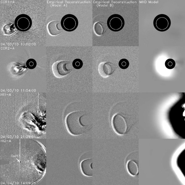
Standard image High-resolution imageFigure 2 shows examples of images from all four of the STEREO telescopes, with Figure 2(a) illustrating STEREO-A's view of the CME and Figure 2(b) showing STEREO-B's perspective. These images demonstrate STEREO's ability to follow the CME continuously from the Sun to 1 AU, though the presence of the Milky Way makes it very difficult to perceive the CME in the HI2-B image. All of the images are displayed in running difference format, with the previous image subtracted from its following image. This is the best technique for subtracting static structures and focusing attention on the dynamic CME material, but it does have the disadvantage of leaving the "shadow" of the previous CME location superimposed onto each image. In any case, the April 3 CME is observed off the east limb of the Sun as seen from STEREO-A and off the west limb from STEREO-B's view. With both STEREO spacecraft having similar lateral perspectives of the event, albeit from opposite sides, the CME appearance in the A and B images is quite comparable.
Download figure:
Standard image High-resolution image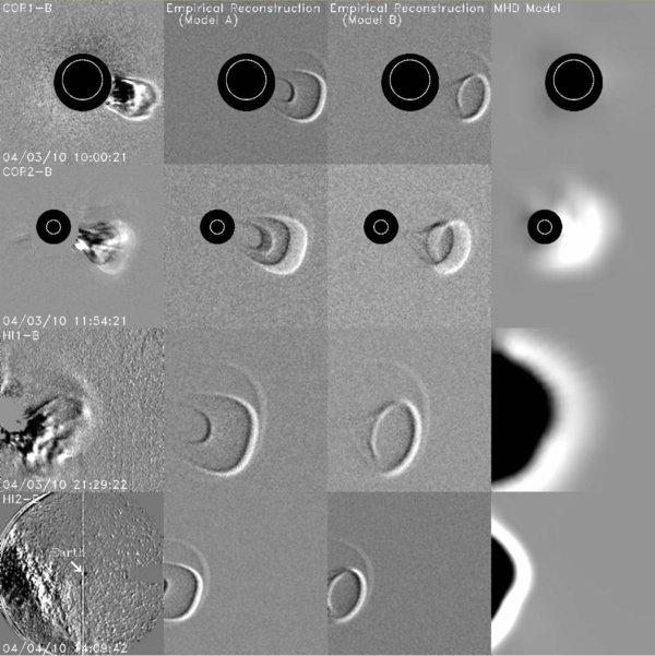
Figure 2. (a) The left panels display STEREO-A images of the April 3 CME, with one image shown for each of STEREO-A's four white-light telescopes. These images are compared with synthetic images computed from three different models of the event. The middle two panels show synthetic images computed from two empirical reconstructions of the CME structure (Models A and B; see Section 4), and the right panels show synthetic images computed from a physical MHD model (see Section 5). The 3 R☉ inner boundary of the MHD model is not close enough to the Sun to allow a synthetic COR1-A image to be computed, so that panel is left blank. (b) Similar to (a), but showing four images from STEREO-B, taken at the same times as the four STEREO-A images in (a). The CME is not apparent in the HI2-B image due to the presence of the Milky Way in the field of view.(An Animation of this figure is available in the online journal.)
Download figure:
Standard image High-resolution imageThe COR1 CME images show two loops, an outer flat-topped loop and an inner more rounded loop. This simple structure becomes more distorted as the CME moves outward into the COR2 and HI1 fields of view, the inner loop in particular becoming harder to discern. The two nested loop appearance in COR1 is consistent with the 3D morphology being that of a tube arcing from a near-equatorial footpoint toward a more southerly one, with the two two-dimensional (2D) loops marking the inner and outer edges of the tube. This picture is consistent with the magnetic flux rope paradigm of CME structure.
One of the fundamental questions about CMEs that the STEREO mission is expected to address is whether magnetic flux ropes lie at the heart of all CMEs. Signatures of CMEs observed by in situ instruments on spacecraft that encounter them in the IPM often have rotating magnetic fields that are suggestive of a magnetic flux rope morphology, defined by a tube-like shape wrapped in a helical magnetic field (e.g., Marubashi 1986; Burlaga 1988; Lepping et al. 1990; Bothmer & Schwenn 1998). But inferring global morphology from single-point measurements is problematic. The LASCO coronagraphs on SOHO have over the years provided numerous outstanding images of CMEs of all sorts, and many can be interpreted as being consistent with a flux rope morphology (Chen et al. 1997; Gibson & Low 1998; Wu et al. 2001; Manchester et al. 2004; Thernisien et al. 2006; Krall 2007). But 3D interpretations of the optically thin 2D white-light CME images are not unique. By observing CMEs from different locations, STEREO can hopefully provide the additional constraints necessary to conclusively demonstrate that tube-shaped structures are truly present in at least some CMEs, which are likely the white-light analogs of the magnetic flux rope signatures detected by in situ instruments.
To date, the STEREO-observed CMEs that have provided the strongest evidence for a flux rope morphology are probably ones from 2008 April 26 and 2008 June 1. Both events eventually struck STEREO-B. Also worthy of mention is a CME from 2007 May 21 that was detected by in situ instruments on MESSENGER near Venus (Rouillard et al. 2009). The in situ observations of the June 1 CME provide one of the best flux rope signatures of any CME in the STEREO era, making this the best example yet of a CME with strong evidence for a flux rope morphology from both imaging and in situ data (Möstl et al. 2009; Wood et al. 2010). The in situ case for a flux rope for the April 26 event is much weaker, but the imaging case for a flux rope shape is particularly strong for this event, as the outline of the flux rope is particularly clear both from a lateral perspective, as viewed from STEREO-A, and from a frontal perspective, as viewed from STEREO-B, which sees the CME as a halo event (Wood & Howard 2009). Thernisien et al. (2009) demonstrate that COR2 images of many other events can be interpreted as being consistent with the flux rope paradigm.
The aforementioned 2008 April 26 CME is particularly relevant here, because it bears some similarity to the 2010 April 3 CME. Both events contain two distinct morphological components. There is a central part of the CME that can be modeled as a flux rope, and there is a front out ahead of this flux rope that can be interpreted as being a compression wave created by the flux rope plowing into slower solar wind material. In Figure 2, the leading compression wave is most visible in the HI1 and HI2 images. It is not visible at all in COR1. Though not clearly visible in the COR2 images in Figure 2 either, hints of it can be discerned in COR2 movies of the CME.
As mentioned in Section 1, the April 3 CME was directed toward Earth and was perceived as a halo CME by SOHO/LASCO at the L1 Lagrangian point near Earth. With both STEREO spacecraft having similar lateral views of the CME, this event is one in which consideration of SOHO/LASCO data is very helpful in assessing the CME's structure, because the halo appearance of the CME from SOHO's perspective is very different from the views of either STEREO spacecraft. Figure 3 shows an image of the event from LASCO's C2 coronagraph. We will describe below how we interpret the bright front expanding south of the Sun as being the outline of a broad flux rope moving toward the observer, but the broad width of the front casts doubt on the initial assumption of a N–S orientation for the flux rope based on the COR1 appearance. Just beyond this front in the C2 image there is a much fainter, more circular halo centered on the Sun that we associate with the leading compression wave. (See Rouillard et al. 2011 for more LASCO images.)
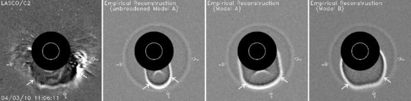
Figure 3. The left panel displays a LASCO/C2 image of the April 3 CME, which is compared with synthetic images computed from three empirical reconstructions of the event (see Section 4). Solid arrows identify the feature we identify with a flux rope, and hollow arrows identify a feature we associate with a compression wave driven ahead of the flux rope. The second panel shows an image computed from a version of Model A assuming a circular cross section for the flux rope, while the third panel shows the actual Model A image computed with an elliptical cross section, which better matches the real image. The third panel displays the synthetic image predicted by Model B.
Download figure:
Standard image High-resolution image3. EMPIRICAL KINEMATIC MODEL
Before attempting to model the 3D morphology of the event in a comprehensive manner considering all available images, it is necessary to understand how the CME expands with time. To this end, we measure the angular distance from the Sun of the top of the flux rope component of the CME in STEREO-A images, throughout its journey from the Sun to the Earth. This provides us with measurements of the elongation angle from Sun center,  . What we really want to know, though, is not but the actual distance from Sun center, r. We compute r using the so-called Fixed-ϕ approximation (Kahler & Webb 2007; Howard et al. 2007, 2008; Sheeley et al. 2008; Wood et al. 2010),
where d is the distance of the observer (STEREO-A in this case) from the Sun, and ϕ is the angle between the CME trajectory and the observer's line of sight to the Sun. This approximation assumes a very narrow CME propagating radially from the Sun in the direction defined by ϕ. Use of Equation (1) requires ϕ to be known. This can be derived from the morphological analysis described in Section 4, which yields ϕ = 65°.
There are two other approximations that we tried as well, the "Point-P" approximation assuming a circular CME centered on the Sun, and the "Harmonic Mean" approximation assuming a circular CME centered halfway between the leading edge and the Sun (Kahler & Webb 2007; Lugaz et al. 2009a; Wood et al. 2010). The best way to decide which approximation works best is to see which leads to constant velocities far from the Sun in the HI2 field of view, where one would expect any CME acceleration or deceleration to have ceased or at least decreased to undetectably low levels. For the 2008 June 1 CME we found that the Harmonic Mean approximation worked best (Wood et al. 2010), but the Fixed-ϕ approximation seems to work best here.
In any case, the top panel of Figure 4 shows the distance versus time measurements for the top of the flux rope. In order to extract velocity and acceleration measurements for the CME, we fit the data points with the same sort of kinematic model that we used to model the 2008 April 26 event (Wood & Howard 2009). This model assumes three kinematic phases: an initial period of constant acceleration, a1, ending at some time, t1; a period of constant deceleration, a2, ending at some time, t2; and finally a period with the CME coasting at a constant velocity. This simple model has only six free parameters, the four mentioned above plus a starting height and a time shift parameter to move the model time grid onto that of the data.
Figure 4. The top panel shows the distance from Sun center of the leading edge of the flux rope component of the 2010 April 3 CME as a function of time. The solid line is a fit to these data points based on a simple kinematic model assuming an initial acceleration phase, a second deceleration phase, and then a constant velocity phase. The bottom two panels show the velocity and acceleration profiles suggested by this fit. Dashed lines indicate the kinematic behavior of the CME front predicted by the MHD model (see Section 5).
Download figure:
Standard image High-resolution imageFigure 4 shows our best fit to the data, indicating an initial acceleration of a1 = 106 m s−2 ending at t1 = 1.73 hr, followed by a deceleration of a2 = −2.32 m s−2 ending at t2 = 37.6 hr. Note that the t = 0 reference time assumed here is the time of the flare quoted in Section 1 (2010 April 3, 9:04 UT). The CME reaches a maximum velocity of 960 km s−1 at a distance of 7.3 R☉ in the COR2 field of view. It then decelerates well into the HI2 field of view, where it reaches its final velocity of 660 km s−1 at 0.73 AU. This speed is in good agreement with the ∼700 km s−1 speed observed for the CME by in situ data near Earth (Rouillard et al. 2011). The deceleration in the IPM is presumably due to drag forces induced by the CME's motion through the slower solar wind.
It is important to emphasize that these measurements are for the top of the flux rope, and not the leading compression wave ahead of it. This wave ultimately becomes brighter and easier to follow than the flux rope in the HI2 field of view, so in the kinematic analysis one has to be careful not to follow it instead of the top of the flux rope. (In the movie version of Figure 2 available in the online journal, a plus sign is used to mark the top of the flux rope to explicitly show what we are tracking.)
4. EMPIRICAL RECONSTRUCTION OF THE 2010 APRIL 3 CME
We reconstruct the 3D structure of the 2010 April 3 CME from the STEREO images following the same prescription used previously to model the 2008 April 26 and 2008 June 1 events (Wood & Howard 2009; Wood et al. 2010). This prescription includes a simple parameterized functional form capable of producing either 3D flux rope shapes or 3D lobular fronts. In this second mode the functional form can reconstruct the leading compression wave of the April 3 CME, and in the first mode it can reconstruct the bulk of the CME behind it that we believe is the flux rope.
The principle here is to construct 3D density distributions within this framework that can be used to compute synthetic images of the CME for comparison with the actual images. The parameters controlling the shape and trajectory of the CME are adjusted to maximize agreement between the synthetic images and the data. This empirical reconstruction is similar in principle to that used by Thernisien et al. (2009) in reconstructing the 3D shapes of 26 CMEs observed by STEREO, but our functional form is more complex and versatile, and we aim to reproduce the CME's appearance in all STEREO images, including HI1 and HI2, whereas Thernisien et al. (2009) focused only on COR2. We ultimately consider SOHO/LASCO data as well.
Our simple prescription for empirical CME reconstruction starts with the computation of a 2D loop in polar coordinates using the following equation:
In order to get a density distribution for a lobular front from this shape, the loop is first converted to Cartesian coordinates, and then densities are mapped onto the 2D grid assuming a Gaussian density profile across the surface:
where δ(x, y) is the distance to the loop from a point within the xy-plane. To allow for an x-dependence for the density, the densities are further modified by
For β>0, densities will increase with distance from the Sun, while for β < 0 they will decrease. Rotating this 2D loop about the x-axis yields a 3D front that can be used to represent structures like the leading compression wave seen in the HI1 and HI2 images in Figure 2.
Flux rope shapes can be computed in a similar fashion. The first step is the computation of not one but two 2D loops using Equation (2), representing the inner and outer edges of the flux rope. This 2D flux rope can be converted into a 3D flux rope by assuming circular cross sections between the inner and outer loops. Densities are then distributed across the surface of the flux rope using Equations (3) and (4), the only difference being that n1 and n2 are in this case already 3D distributions instead of 2D.
The final step is to rotate our front and flux rope to the desired directions. This means defining a longitude and a latitude (lF, bF) that indicate the direction of the front and/or flux rope in a heliocentric aries ecliptic coordinate system (as shown in Figure 1). Unlike the leading front, the flux rope component is not rotationally symmetric, so the flux rope requires an additional orientation angle, ϕfr, defining the orientation of the flux rope with respect to the ecliptic plane. After all the rotations are applied, the flux rope and leading front are combined into a single density cube, which can then be used to compute synthetic images. The scale size of the density cube as a function of time is established according to the kinematic model from Section 3 (see Figure 4). We assume a simple radial, self-similar expansion of the CME, allowing the same density cube to be applicable at all times.
The synthetic images are generated using a white-light rendering routine to perform the necessary calculations of Thomson scattering within the density cube (Billings 1966; Thernisien et al. 2006; Wood et al. 2009b). As mentioned above, we adjust the parameters of the model to maximize the agreement between the synthetic and actual images. Given the substantial number of STEREO images, this means that in practice we compare real and synthetic movies of the CME as it progresses from close to the Sun in COR1 all the way out to 1 AU and beyond in HI2.
The parameters of our best-fit model are listed in Table 1. The rmax and nmax parameters are simply normalized to 1 for the leading front, and other distances and densities are given relative to these values. A normalized distance is necessary, as it is the kinematic model in Figure 4 that actually provides an absolute size scale as a function of time. As for the density, we are here interested purely in reproducing the appearance of the CME in the STEREO and LASCO images and not its precise brightness, so we do not bother with absolute density values. The trajectory of the flux rope component defined by lF and bF corresponds to a direction 2°W of Earth and 16°S (i.e., S16W02), only about 11° from the direction expected from the flare site (S23W11).
Table 1. CME Morphological Parameters
| Quantity | Front | Flux Rope | ||
|---|---|---|---|---|
| (Outer Edge) | (Inner Edge) | |||
| rmax | 1 | 0.95 | 0.63 | |
| σ (deg) | 42.5 | 27.6 | 21.2 | |
| α | 3.3 | 3.0 | 4.0 | |
| nmax | 1 | 4.29 | ||
| σn | 0.0085 | 0.0085 | ||
| β | 3 | 3 | ||
| ϕfr (deg) | ⋅⋅⋅ | −80, 10a | ||
| ηfr | ⋅⋅⋅ | 1.6 | ||
| lF (deg) | 195 | 195 | ||
| bF (deg) | −8 | −16 | ||
Note.a The flux rope orientation is ϕfr = −80° for Model A and ϕfr = 10° for Model B.
Download table as: ASCIITypeset image
Figures 2 and 3 show synthetic images computed from this reconstruction, which in the figures can be compared with the actual images. The synthetic images are displayed in the same running difference format as the real images, and we have added random noise to the synthetic data. In the online version of this paper we present a movie version of Figure 2. This not only provides a more thorough data–model comparison, but in movies it is much easier to perceive the CME in the HI2 images, where it is quite faint. There are clearly some changes to the CME's appearance as it moves away from the Sun, but the self-similar expansion assumption used here seems to be a reasonable approximation. This was also the case for the 2008 April 26 CME, but not the case for the 2008 June 1 event, which required a time-dependent morphology (Wood et al. 2010).
The second column in Figure 2 shows our model of the CME assuming a nearly N–S orientation for the flux rope (ϕfr = −80°, to be precise), which we call Model A. This was the orientation we inferred from the COR1 appearance of the CME (see Section 2). However, problems develop when the model is compared with the LASCO data. The second panel of Figure 3 indicates how Model A predicts that LASCO should see the flux rope as a relatively narrow front extending south of the Sun (marked by two solid white arrows). There is such a front in the actual C2 image, but it is much broader than Model A initially predicts.
The only way to solve this problem is to abandon our assumption of a circular cross section for the flux rope and allow it to have an elliptical profile. We do this by simply stretching the flux rope perpendicular to its plane of orientation by a factor of ηfr = 1.6, so the broadening factor ηfr becomes an additional parameter for the flux rope shape that we list in Table 1. The third panel of Figure 3 shows that this leads to much better agreement with the LASCO/C2 image. This change in the flux rope shape has almost no effect on the appearance of the CME from the perspective of the two STEREO spacecraft, as their lateral views provide little depth perception in the direction along which the flux rope was broadened.
However, we find that the increased degree of freedom involved in allowing non-elliptical flux rope cross sections complicates our ability to infer the orientation of the flux rope from the images. In this modified flux rope paradigm, we find that we can also reproduce the STEREO and LASCO images reasonably well with a flux rope oriented E–W instead of N–S. We call this Model B, which assumes ϕfr = 10°, a 90° rotation from the Model A flux rope. Figure 5 shows the 3D structures of both Model A and Model B. The only difference between the flux rope morphologies of these two models lies in the 90° rotation quantified by the ϕfr parameter.
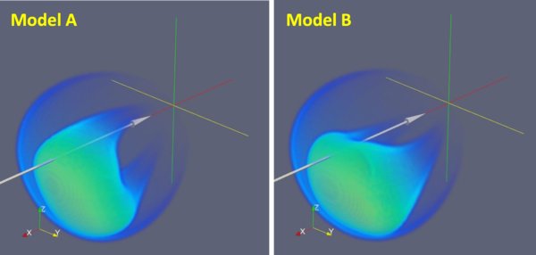
Figure 5. Two models of the density distribution of the April 3 CME. The xy-plane is the ecliptic plane. The arrow indicates Earth's trajectory through the CME structure.
Download figure:
Standard image High-resolution imageThe third column of Figure 2 and the fourth panel of Figure 3 illustrate the synthetic images predicted by Model B. Model B reproduces the LASCO/C2 image at least as well as Model A, and may even be better in reproducing the CME appearance in the COR2 and HI1 images. It is only in the COR1 images that Model A is clearly superior. In Model A, the southern LASCO/C2 front is assumed to be the outline of the southern leg of the flux rope, while in Model B it is the outline of the southern side of the flux rope. Overall, we find it impossible to decide which of these two models is preferable based on the imaging data alone, so we present both interpretations here. The one conclusion that seems unavoidable is that if the central part of the CME that we have been modeling as a flux rope is indeed a flux rope, it cannot have a circular cross section. It must be significantly elliptical.
Various analyses of in situ data have suggested that the data are often best explained by flux ropes that are flattened in their propagation direction, a picture consistent with the predictions of many MHD models (e.g., Mulligan & Russell 2001; Vandas et al. 2002; Manchester et al. 2004; Riley & Crooker 2004; Démoulin & Dasso 2009). This flattening is expected to occur as the CME plows through the ambient solar wind in the inner heliosphere. Our inference of an elliptical cross section for the April 3 CME is generally consistent with this picture, but our analysis indicates that the flux rope channel of the April 3 CME is elliptical right from the start, and does not simply acquire its ellipticity during its journey through the IPM.
Analogous to our difficulty deciding between Models A and B, Thernisien et al. (2009) also reported significant uncertainties in the orientation of many of the flux rope CMEs that they analyzed with STEREO. In general, the orientation should be better defined for narrow flux ropes, in which the CME extent along the axis is much greater than in the transverse direction. This is the case for the April 26 CME (Wood & Howard 2009), but is certainly not the case here. Both our flux rope models present a similar, squarish visage from a frontal perspective (see Figure 5). We would also emphasize that inferring a CME's underlying magnetic structure from images will always require that mass be loaded into the structure in such a way as to outline it in the images. Clearly that has not happened well enough here to allow for a unique interpretation.
In principle, in situ observations of flux rope CMEs in the IPM can be used to infer an orientation for the flux rope, and this CME was in fact observed in situ by the ACE and Wind spacecraft when it reached Earth. Unfortunately, Möstl et al. (2010) found that even though the in situ signature of the CME fulfils many of the criteria of a magnetic cloud (Burlaga et al. 1981), the magnetic field signature cannot be fitted well with either a force-free or Grad–Shafranov flux rope model, so no clear orientation can be inferred. They infer a total size of ∼0.4 AU for the magnetic cloud-like region. This sizable distance agrees well with what we would expect based on Model A, which predicts a lengthy path for the Earth through the CME, since it has the Earth traveling down the northern leg of the flux rope (see Figure 5). In contrast, Model B, which has the Earth merely skimming the northern edge of the elliptical flux rope channel (see Figure 5), suggests a much smaller encounter region of only ∼0.2 AU.
Figure 6 shows a magnetogram of the source region for the April 3 CME, from the Michelson Doppler Imager (MDI) instrument on SOHO (Scherrer et al. 1995). A solid line is used to estimate the neutral line orientation of this active region, and this is compared with the flux rope orientations suggested by our two reconstructions of the CME, Model A and Model B. The former implies that the flux rope is roughly parallel to the neutral line. This would be consistent with previous work that has found that flux rope orientations inferred from either in situ data or coronagraphic imaging are usually oriented roughly parallel to the filament channels and/or source region neutral lines (Bothmer & Schwenn 1998; Zhao & Hoeksema 1998; Cremades & Bothmer 2004; Yurchyshyn et al. 2006; Démoulin 2008).
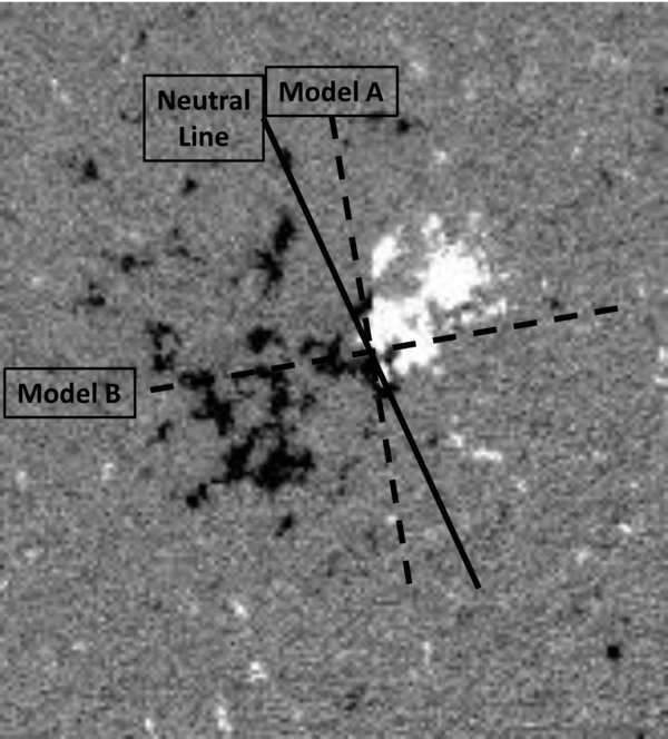
Figure 6. SOHO/MDI magnetogram of the active region that is the source region of the April 3 CME, taken shortly before the flare that accompanies the CME. The solid black line is an estimate of the neutral line of the active region. The dashed lines show two very different orientations of the flux rope suggested by two distinct empirical reconstructions of the April 3 CME (Model A and Model B).
Download figure:
Standard image High-resolution imageThere are exceptions, though (e.g., Zhao & Hoeksema 1998; Webb et al. 2000), and it is particularly relevant to point out that the 2008 April 26 CME, which we have argued is similar to the 2010 April 3 CME in appearance and kinematics, is one of these exceptions. The STEREO observations of the April 26 event clearly show that the flux rope of that CME inferred from the white-light imaging is perpendicular to the neutral line of the source region (Wood & Howard 2009; Cheng et al. 2010). Our Model B of the 2010 April 3 event would be consistent with that geometry. One difference between the April 26 and April 3 events that might be relevant here is that only the April 3 event's source region actually has a filament along the neutral line, which erupts along with the CME. There is no clear filament marking the neutral line of the April 26 CME's source region.
More flux rope CMEs with well-defined orientations from STEREO data would be helpful to better address the connection between flux rope orientation and underlying photospheric magnetic field topology. But our struggle to find a truly unique flux rope morphology for the April 3 CME despite constraints from three different observatories in three very different locations illustrates the difficulties. Without a unique solution, it is not even possible to claim with any great confidence that our analysis has demonstrated that a visible flux rope is actually the best interpretation of this CME's appearance. At the very least, the case is not nearly as convincing as that for the 2008 April 26 and 2010 June 1 CMEs (Wood & Howard 2009; Möstl et al. 2009; Wood et al. 2010). Even if only CMEs that are well observed from multiple perspectives are considered, apparently only a fraction will present an appearance revealing a flux rope's presence in a truly unambiguous manner.
Although the flux rope paradigm seems shaky for the April 3 CME with regard to both its visual and in situ signatures, it is not clear to us that any other simple existing model would do any better. There are, for example, various spheromak conceptualizations that envision CMEs as being toroids of magnetic field traveling outward from the Sun (Ivanov & Harshiladze 1985; Vandas et al. 1993, 1998). The usual argument against detached spheromak structures is that without connection to the Sun they cannot explain the counterstreaming electrons often observed during in situ encounters with CMEs. From an imaging perspective, many if not most CMEs show visual evidence for lines of connection back to the Sun, including this one (see Figure 2). However, a "tethered spheromak" picture (Gibson & Low 1998, Gibson & Fan 2008) could conceivably resolve this issue and in principle do no worse than we have done here operating within the flux rope paradigm.
5. PHYSICAL MODELING OF THE 2010 APRIL 3 CME
The empirical reconstruction procedure discussed in the last section is a very useful way to try to interpret CME imaging data, but there is little or no physics in this process. To provide greater physical insight into the nature of this CME and its propagation through the IPM, we also present here a numerical model of the event, computed using a procedure developed by Wu et al. (2007a, 2007b). This model combines the Hakamada–Akasofu–Fry (HAF) code (version 2; Fry et al. 2001), which computes the solar wind's evolution out to 18 R☉, and a fully 3D MHD code that then carries the simulation out to 285 R☉ (Han et al. 1988). The inner boundary conditions for the HAF part of the code are derived from solar magnetograms and resulting source surface maps using the procedures of Arge & Pizzo (2000).
The model as described above establishes the characteristics of the steady, quiescent solar wind into which the April 3 CME propagates. The CME itself is produced by introducing a pressure pulse at the inner boundary, at the time and location of the flare associated with the event (i.e., at 9:04 UT, at a position S23W11 relative to the Sun–Earth axis). The pressure pulse consists of a 54 minute exponential rise in wind velocity to a peak of 900 km s−1, followed by a 54 minute exponential decay back to the original value. Note that this MHD simulation was not done as a real-time prediction test, but with the magnitude of the velocity pulse adjusted to make the resulting CME front arrive at Earth at the observed time of 7:58 UT on April 5.
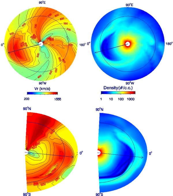
Figure 7 shows velocity and density maps suggested by this model at 17:00 UT on April 5, about 9 hr after the CME first reaches Earth. Because the model provides 3D density distributions in the inner heliosphere, we can use these densities to compute synthetic STEREO images, just as we did for the density distributions derived from the empirical reconstruction process described in Section 4. The last column of Figure 2 shows these synthetic images. No COR1 images are shown, as the COR1 field of view resides mostly inside the inner boundary of the model. The synthetic COR2 images suffer somewhat from a lack of sufficient spatial and time resolution (1 R☉ and 1 hr, respectively) in that field of view. Figure 2 represents one of the first side-by-side comparisons of real STEREO images and synthetic images computed from a numerical model of the inner heliosphere. Lugaz et al. (2009b) previously used the Space Weather Modeling Framework (SWMF) package (Tóth et al. 2005) to model a pair of interacting CMEs observed very early in the STEREO mission in 2007 January. Odstrcil & Pizzo (2009) present synthetic HI2 images of STEREO-observed CMEs using their ENLIL code, but the actual HI2 observations of those events are shown elsewhere.
Figure 7. Numerical model of the 2010 April 3 CME's propagation into the IPM, at April 5, 17:00 UT about 9 hr after encountering Earth. The upper two panels show the velocity and density distribution in the ecliptic plane. The circle indicates Earth's orbit, with Earth on the left at 0°. The bottom two panels illustrate the velocity and density distribution in a meridional plane. A circle is drawn to indicate at 1 AU from the Sun. The Earth would be to the right on this circle at 0°.
Download figure:
Standard image High-resolution image
Since there is no real structure to the model CME, the numerical model obviously cannot match the observed CME's internal appearance. It is more relevant to compare the model CME front with the shape of the leading compression wave of the observed CME, and the model does not do too bad a job in that respect. For one thing, the model is able to reproduce the somewhat flattened appearance of the CME front in the southern half of the HI2 field of view. (See both the lower panels of Figure 7 and the synthetic HI2 images in Figure 2.) The direction in which this flattening is seen corresponds to the location of the heliospheric current sheet, where ambient solar wind velocities are somewhat lower than above and below the sheet. The lower velocities inhibit the expansion of the CME front somewhat, producing the flattening, which we believe is consistent with the observations. (As always, the faintness of structures in the HI2 images makes it advantageous to refer to the movie version of Figure 2 in the online journal.)
Another instructive exercise that we can perform with the numerical model is to compare the kinematics of the model CME front with that of the real one, as shown in Figure 4. In order to define the model front's radial distance as a function of time, we fit a Gaussian to the front's radial density profile. This leads to the dashed line in the top panel of Figure 4. The limited spatial resolution of the model and the manner in which the numerical CME is launched lead to a front significantly broader than the real one. This is the reason the numerical CME distances are significantly below the real distances at early times in the COR2 and lower HI1 fields of view.
In order to infer velocities and accelerations for the model CME, we first fit an eighth-order polynomial to its distance versus time curve in order to smooth out some of the small-scale "noise" associated with uncertainties in the Gaussian fitting procedure. The CME velocity is then computed from this polynomial fit, and the result is displayed as a dashed line in the middle panel of Figure 4. Finally, CME accelerations are inferred from the time-dependent velocity measurements in a similar fashion.
It is encouraging that the ∼900 km s−1 CME velocity close to the Sun inferred from the model agrees well with that observed in the data. Furthermore, both the model and observations indicate similar amounts of deceleration for the CME front during its IPM travel to 1 AU, leading to a front velocity at Earth of about 700 km s−1, consistent with in situ observations of the CME from ACE and Wind (Möstl et al. 2010; Rouillard et al. 2011). This would support the use of numerical models such as this for inferring CME IPM decelerations in real time, potentially improving 1 AU arrival time predictions for space weather forecasting purposes.
6. SUMMARY
Using STEREO and SOHO/LASCO observations, we have performed a detailed analysis of the 3D structure and kinematics of the first geoeffective CME of solar cycle 24, which was launched from the Sun on 2010 April 3. This analysis has two parts: an empirical reconstruction and a computational model. Our findings can be summarized as follows.
- 1.Morphologically the CME consists of two distinct parts, a bright, central structure and a leading front ahead of it that we interpret as a compression wave created by the fast CME plowing into slower ambient solar wind. Our kinematic model of the CME indicates that the CME reaches a maximum velocity of 960 km s−1 in the COR2 field of view and then gradually decelerates in the IPM until it reaches a final coasting velocity of 660 km s−1 at 0.73 AU, consistent with velocities observed for the CME by the ACE and Wind spacecraft near Earth.
- 2.The bright central structure of the CME is reasonably well matched by a 3D flux rope shape, but the case for such a flux rope geometry is not as strong as for the 2008 April 26 and 2008 June 1 CMEs that we have analyzed in the past (Wood & Howard 2009; Wood et al. 2010). We cannot infer a unique orientation for the flux rope. A model with a nearly N–S orientation (Model A) best explains the CME's appearance at early times in COR1 images, while a more E–W orientation (Model B) seems to work better at later times, especially in HI1. Regardless of orientation, a flux rope shape reproduces the STEREO and SOHO/LASCO images collectively only if the flux rope has a very elliptical cross section, flattened in the radial direction of propagation from the Sun.
- 3.The CME is directed 2°W and 16°S of Earth, with Earth being hit by either the northern leg of the flux rope (Model A) or the top of the apex of the flux rope (Model B), as shown explicitly in Figure 5.
- 4.The numerical model of the CME is reasonably successful in reproducing the shape of the observed compression wave of the CME. Of particular note is a flattening of the front in the south that the model suggests is due to the presence of the heliospheric current sheet (and therefore lower ambient solar wind speeds) at that location. The model is able to approximate the observed velocity of the CME both close to the Sun and at 1 AU, meaning that it is doing a reasonable job of reproducing the amount of deceleration experienced by the CME in the IPM due to interaction with the ambient solar wind.
This work has been supported by NASA award NNH10AN83I to the Naval Research Laboratory. The STEREO/SECCHI data are produced by a consortium of NRL (US), LMSAL (US), NASA/GSFC (US), RAL (UK), UBHAM (UK), MPS (Germany), CSL (Belgium), IOTA (France), and IAS (France). In addition to funding by NASA, NRL also received support from the USAF Space Test Program and ONR. We have also utilized data from the LASCO and MDI instruments aboard SOHO, which is a project of international cooperation between ESA and NASA.