


ABSTRACT
This paper reports the extension of a previously reported experimental method for the identification and characterization of astrophysical weeds in millimeter and submillimeter spectra to the widely used 210–270 GHz atmospheric window. At 300 K, these spectra contain contributions from approximately 40 vibrational states in addition to the cataloged ground state. The quantum mechanical analysis of such a large number of states would be a formidable challenge due to the complex interactions among these dense vibrational states. A new heterodyne receiver-based system is reported, as well as its intensity calibration. Results are presented in the standard astrophysical catalog format as well as our previously described point-by-point format that is effective for the characterization of blends. We also describe and validate an additional spectral synthesis approach, based on the much smaller line list catalog, which is useful in the blended line limit.
Export citation and abstract BibTeX RIS
1. INTRODUCTION
Advances in the sensitivity and angular resolving power of millimeter and submillimeter telescopes (Becklin 2005; Clery 2009; Turner & Wooten 2006) are rapidly outpacing the spectroscopic database, especially as they make possible more detailed studies of regions such as hot molecular cores. There is a strong consensus that the major contributors to this spectroscopic challenge are the spectra of difficult to analyze, low-lying vibrational states that are excited at these temperatures, the so-called astrophysical weeds (Goldsmith et al. 2006).
We have recently proposed (Medvedev & De Lucia 2007) and demonstrated (Fortman et al. 2010a) an alternative approach to the usual quantum mechanical (QM) assignment and analysis procedure used to calculate line lists for astrophysical catalogs (Muller et al. 2005; Pickett et al. 1998). This approach uses intensity-calibrated millimeter and submillimeter spectra, taken at several hundred different temperatures, to calculate the astrophysically important lower state energies and transition strengths of observed lines, without the need for QM assignment.
In this paper, we describe the application of this approach to ethyl cyanide in the widely used 210–270 GHz region. This allows us to compare the results with our earlier study of this same molecule in the 570–645 GHz region. We also describe a new synthesis approach of particular use in crowded and blended spectral regions. In the 210–270 GHz region, only 317 of the 3096 strongest lines in the experimental spectrum are in the catalogs, while 936 of the lines in the catalogs are not among the 3096 strongest experimental lines. Figure 1 shows a more detailed comparison.

Figure 1. Absorbance of the 3096 strongest experimentally observed lines (upper black trace) and that of the 517 strongest catalog lines (lower red trace) for the ethyl cyanide spectrum between 210–270 GHz, both sorted by strength. The points plotted are so dense as to make each family of points appear as a continuous line.
Download figure:
Standard image High-resolution imageWe have also completed similar experimental work for seven other well-known astrophysical weeds: methyl formate, acetaldehyde, dimethyl ether, methanol, sulfur dioxide, methyl cyanide, and vinyl cyanide. Preliminary analyses show similar results for all species except SO2, whose simpler spectroscopy has led to a more complete spectral database.
The excited vibrational states of ethyl cyanide are difficult to analyze partially because there are so many of them (the results reported in this paper include contributions from about 40 different vibrational states) and especially because many, if not most, excited vibrational states are mixed and perturbed by other nearby states. The lowest lying vibrational states are ν21 at 222 cm−1, ν13 at 226 cm−1, ν20 at 378 cm−1, and the combinations 2ν21, 2ν13, and ν21 + ν13 near 450 cm−1 (Heise et al. 1981). Some of the lines in ν21 and ν13 have been identified (Brauer et al. 2009) and used to assign lines from the interstellar medium (Mehringer et al. 2004), but the more perturbed lines have been a bigger challenge and thus these vibrational states are as yet not included in the catalogs.
Figure 1 can be understood in the context of this vibrational state structure. Since ethyl cyanide is a semi-rigid molecule, the rotational structure in these excited states can be expected to approximate that of the ground state. Under this assumption, in the intensity sort of Figure 1, it would be expected that the strongest lines not included in the catalog would be in the ν21 and ν13 vibrational states and that they would be weaker than the strongest ground state lines by the vibrational Boltzmann factor, ∼3 at 300 K. Inspection of Figure 1 shows that this expectation is realized.
An important astrophysical question is how this factor varies as a function of temperature. As is well known, interstellar temperatures vary widely, with many being at very low temperatures. However, with the ability of arrays to resolve smaller hot cores, much higher temperatures have been observed. For example, with the Submillimeter Array a rotational temperature of 578 ± 134 K has been measured for ethyl cyanide in G19.61–0.23, with similarly high temperatures for other species (Qin et al. 2010). Presumably with the high angular resolving power of ALMA even smaller and hotter cores will be observed. Accordingly, Figure 2 shows these intensity factors over the 100–500 K range both for the excited states near 200 cm−1 and the complex of states around 400 cm−1. The results are a very steep function of temperature. At 100 K, the strongest lines not included in the spectra are weaker by a factor of ∼20, but those due to the states around 400 cm−1 are weaker by a factor of ∼400. Thus, the inclusion of an analysis that contains the states near 200 cm−1 would make the catalog rather complete at 100 K. However, at 500 K, even the states around 400 cm−1 would contribute lines whose intensities were reduced by only a factor of ∼4.

Figure 2. Boltzmann population factors for the ν21 and ν13 vibrational states near 200 cm−1 and the ν20, 2ν11, 2ν13, and ν11 + ν13 around 400 cm−1.
Download figure:
Standard image High-resolution image2. EXPERIMENTAL
2.1. The Spectrometer
The spectrometer used in this work is based on a synthesized ×24 frequency multiplied probe, with a heterodyne receiver, coupled to a temperature-controlled 6 m long cell. The temperature of the cell (Fortman et al. 2010a) was slowly ramped from 240 K to 385 K over a period of 295 minutes. During this period, 437 spectral scans were recorded. Each scan measured the spectral intensity at 25 kHz intervals, with an integration time of ∼15 μs bin−1 and a total scan time of 40 s. The temperature variation over each scan was small enough that the assumption of a constant temperature did not significantly impact the error budget of the experiment.
The microwave spectrometer is described in a recent publication (Medvedev et al. 2010). Because an analysis of the experimental spectrum, without QM assignment, is the product of this work, it is important that this system not have spurious responses. These are most likely at multiples of the 8.75–11.25 GHz drive frequency of the ×24 multiplier chain. In our earlier work in the 570–645 GHz band, spurious responses were below 5 × 10⁻⁴, even with the use of a broadband detector. However, the broader fractional bandwidth of the ×24 probe system (25% versus 12.5%) resulted in unacceptably large (∼5%) power at ×23 and ×25 of the drive frequency. The use of the frequency selective heterodyne receiver reduced these spurious responses to a level well below the weakest lines reported here.
2.2. Intensity Calibration
A foundation of spectroscopy in the millimeter and submillimeter is that it is possible to use the sharpness of spectral features to separate them from wider system variations in power. However, this ordinarily sacrifices knowledge of absolute power and often modifies lineshapes as well. In our system, we directly measure the output of the intermediate frequency (IF) detector to provide a DC-coupled measure of power.
After using an automated procedure to cut each spectral line from the data, we use a spline fit to interpolate across each region that contains one or more spectral lines (Fortman et al. 2010a). The resulting line-free spectrum is subtracted from the signal channel spectrum to remove the baseline. This is done individually for each of the 437 temperature scans because the baseline is a function of temperature. Finally, to produce the absolute intensities, the spectrum is normalized by dividing by the channel that preserves the DC power levels.
As in our earlier work, we used the intensity residuals of our temperature calibration fit (see Sections 3 and 4) as a measure of the accuracy of the intensity calibration. While we expected that the more conventional electronic detector approach of the 210–270 GHz system would be more linear than the helium temperature bolometer used in our earlier work, this did not prove to be the case. However, we found that by calibrating the response of the IF amplifier–diode detector combination and by attenuating the probe power by ∼100, that excellent (∼1%) intensity calibration could be obtained. Inspection of the spectra showed that they contained about 1% vinyl cyanide. However, because of the intensity calibration and well-defined Doppler linewidths it was straightforward to subtract this spectrum to high accuracy.
3. ANALYSIS
We have previously reported the general approach of our method (Medvedev & De Lucia 2007) as well as the specific procedures (Fortman et al. 2010a). Briefly, we selected 105 assigned lines that are included in the cataloged output of QM analyses (Muller et al. 2005; Pickett et al. 1998) to use as references. All of the lines chosen as reference lines are a-type lines, thereby avoiding the issues associated with the ambiguity of the size of the b-type transition moments for this molecule (Fortman et al. 2010a; Heise et al. 1974; Laurie 1959). Since these reference lines have known strengths Sijμ2 and lower state energy levels El from the QM analyses, and Doppler widths δνD and line frequencies ν0 from the known temperature and measured frequencies of our experiment, we can use a fit of their measured peak absorbance,
to obtain the spectroscopic temperature T and nL/Q, where n is the number density of the molecules, L is the effective path length of the spectroscopic cell, and Q is the molecular partition function. This fit is preformed for each of the 437 spectra obtained over the temperature range 240–385 K.
Because we are at a lower frequency than in our earlier work, we found that even at 0.5 mTorr there was a small contribution from pressure broadening to the observed linewidth. Since this contribution was small and because in heavy molecules such as ethyl cyanide there is little state dependence for pressure broadening, we accounted for the impact of varying linewidth on the peak absorbance by introducing a factor of  into Equation (1). With ν in MHz, the fit for this term yielded k = −57,333 MHz, corresponding to about a 5% effect across each spectrum.
Next we use two complimentary analysis procedures, both based on Equation (1), to provide the astrophysically meaningful data. Because most lines of significant intensity are included in the QM catalog at 77 K, for the point-by-point analysis of Section 3.2 we take advantage of this fact to include in our analysis a 77 K spectrum calculated from the QM analysis.
3.1. A Line List Catalog
In the first approach, after a peak finder locates the individual lines, they are fit to Gaussian lineshape functions, producing a line list of frequencies, line strengths, and linewidths. In congested areas multiple Gaussians are fit simultaneously. Software then collects the information for each of the 3096 lines and performs a least squares fit as a function of the 437 temperature scans to determine Sijμ2 and El for each of the lines, both assigned and unassigned. This produces the usual astrophysical catalog data. Because of the possibility of blends, this software also provides figures of merit to inform the user of spectral features whose origins may be from more than a single transition. As we have previously noted, these blends are a problem not only for this approach, but also for the usual QM catalog approach because a number of cataloged lines are overlapped by significantly stronger lines that are not included in the catalogs. In Section 4.3, we demonstrate a simulation strategy that minimizes the effect of these blends and overlaps.
3.2. A Spectral Point-by-point Catalog
The second approach makes no attempt to identify and characterize individual lines, but rather seeks to predict, on a point-by-point basis, the spectra as a function of temperature. Because of the exponentials in the Gaussian lineshape and in the lower state energy term, the absorbance as a function of frequency can be recast as

with the Doppler width (HWHM) given by
where Na is Avogodro's number and M is the molecular mass.
The absorbance normalized by the nL/Q factor then becomes
with
According to Equation (4) every frequency slice of the data (437 points, one for each temperature) can be represented by two parameters  ijμ2 and
  . On line center, when ν = ν0,
  equals the lower state energy, while
  ijμ2 corresponds to the line strength. Off line center, the meanings of
  ijμ2 and
  are less physical, but Equation (4) is still a valid fitting function for describing the spectral intensity for an unblended line.
4. RESULTS
Figure 3 shows small portions of the experimental spectrum of ethyl cyanide, along with predictions from analyses described below. In areas that contain many closely spaced lines, especially of varying strengths, it is harder to remove the baseline. The region between 224.41 GHz and 224.51 GHz is an example of one of the more difficult regions. The fact that the experimental trace goes negative around the weak lines near the strong line at 224.460 is indicative of an error in the baseline normalization. However, these errors for a challenging region are less than 2% of the strength of the strongest lines. Moreover, both the catalog Gaussian fit and the point-by-point fit suffer less from this problem, in all likelihood because of the aforementioned averaging over the 437 spectral scans.
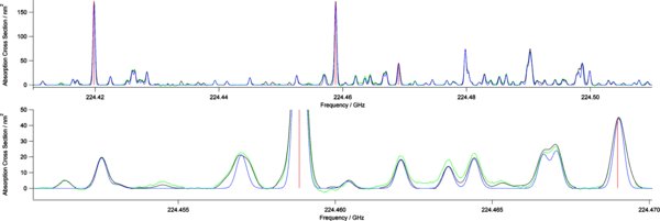
Figure 3. Portion of the ethyl cyanide spectrum between 224.41 and 224.51 GHz at 300 K. The green trace is a single scan at 300 K, the blue scan is a simulation based on all of the 3096 catalog lines, and the black trace a simulation based on the point-by-point analysis of the 437 temperature scans. The red stick spectra represent the lines that are included in the QM catalogs.
Download figure:
Standard image High-resolution imageTable 1 shows examples of the measured spectroscopic temperatures and nL/Q parameters for 10 of the 437 spectral scans. These are included in the archives available in the online journal along with the experimental data for each temperature. Each spectral file consists of 2.4 million absorbances, starting at 210 GHz and incrementing in steps of 25 kHz. We include these files so as to make the results below traceable to the data on which they are based and to make possible alternative or more extended analyses in the future. Because they are intensity calibrated, an unusual attribute in the millimeter/submillimeter, and variable temperature, they should also be of considerable utility in the extension of QM analyses to higher vibrational states (Fortman et al. 2010b).
Table 1. Experimental Temperatures and nL/Q Parameters for 10 of the 437 Spectral Scans
| Index | T (K) | nL/Q (nm−2) |
|---|---|---|
| 50 | 250.474 | 0.0014179 |
| 51 | 250.783 | 0.0014089 |
| 52 | 251.279 | 0.0014006 |
| 53 | 251.552 | 0.0013920 |
| 54 | 251.779 | 0.0013842 |
| 55 | 252.144 | 0.0013777 |
| 56 | 252.261 | 0.0013709 |
| 57 | 252.645 | 0.0013640 |
| 58 | 253.228 | 0.0013574 |
| 59 | 253.265 | 0.0013479 |
Only a portion of this table is shown here to demonstrate its form and content. A machine-readable version of the full table is available.
Download table as: DataTypeset image
4.1. The Catalog Results
Table 2 shows the results for 13 of the 3096 lines analyzed in this work in the catalog format described in Section 3.1. As described in our earlier work (Fortman et al. 2010a), this table includes a column that tags potentially unreliable results according to "W" (a line that is too wide in comparison to its expected Doppler width), "G" (a line whose Gaussian fits did not converge), and "T" (a line whose temperature dependence is unphysical). The full table is available in the electronic archives of this journal. While these tags are primarily designed to find problems associated with blends, they also serve to highlight problems in the highly automated analysis of a very large amount of spectral data.
Table 2. Example of the Results of This Work in Catalog Format
| Frequency | Sijm2 | Energy | Figures of Merit |
|---|---|---|---|
| (MHz) | (D2) | (cm−1) | |
| 242319.392 | 126 | 376 | |
| 242319.852 | 743 | 480 | |
| 242320.76 | 427 | 558 | |
| 242324.984 | 157 | 383 | |
| 242325.414 | 488 | 397 | |
| 242331.441 | 329 | 616 | W |
| 242332.629 | 417 | 804 | W, T |
| 242334.097 | 250 | 427 | |
| 242334.513 | 400 | 473 | |
| 242336.997 | 316 | 791 | W |
| 242339.645 | 368 | 576 | |
| 242348.834 | 348 | 709 | |
| 242349.364 | 380 | 687 |
Only a portion of this table is shown here to demonstrate its form and content. A machine-readable version of the full table is available.
Download table as: DataTypeset image
To provide a measure of the physical basis of this approach, we compared both the lower state energies and transition strengths obtained from the experimental data with the results of the QM calculations. As expected, the accuracy is related to the experimental absorbances, both because of the experimental noise in the system and the impact of uncataloged overlapping lines on this comparison. Of the 317 lines that exist both in the catalogs and in our spectra, for the 74 strongest lines the rms difference is 8.4 cm−1 in their lower state energies and for the 134 strongest lines the rms difference is 10.4 cm−1 in their lower state energies. Although it is difficult to evaluate the impact of overlaps on this comparison, a reasonable elimination of lines suspected to be due to overlap results in a large majority of the differences being <50 cm−1. Most of the larger of these are due to the weakest of the 317 lines.
4.2. The Point-by-point Results
Table 3 shows a subset of the 2.4 million pairs of  ijμ2 and
  coefficients of Section 3.2. The complete set is available in the electronic archives of this journal. In it
  ijμ2 is reported in units of D2 (Debye squared) and
  in units of cm−1. To provide an easy way to calculate the absorbance scaled by the nL/Q parameter at an arbitrary temperature using archived
  ijμ2 and
  coefficients, we reformulate Equation (4) as
with
and M the molecular weight in amu, T the temperature in K, and ν the frequency in MHz.
Table 3. Parameters of the Point-by-point Fit
 |
 |
|---|---|
| (D2) | (cm−1) |
| 206.104 | 962.644 |
| 280.137 | 982.967 |
| 316.401 | 967.523 |
| 388.789 | 971.572 |
| 447.064 | 962.762 |
| 458.688 | 934.691 |
| 549.453 | 941.656 |
| 610.615 | 936.118 |
| 605.825 | 908.508 |
Only a portion of this table is shown here to demonstrate its form and content. A machine-readable version of the full table is available.
Download table as: DataTypeset image
Because this approach is based on frequency points, not spectral lines, there is no explicit line count. However, there are more than 9500 features at 300 K with signal-to-noise ratio greater than 2 and whose absorbances are greater than 0.001. This number is larger than the 3096 lines included in the line-by-line catalog in part because the fitting procedure effectively averages over the 437 spectra. This not only reduces the random noise in the spectrum, but also improves the spline baseline subtraction because much of the baseline varies as a function of temperature over the 437 spectral scans. Because of the rapid growth of the density of vibrational states with energy, these 9500 lines have their origins in approximately 40 vibrational states. Some of the lines in this analysis are also due to the 13C isotopic species.
4.3. An Alternative Method for the Use of the Catalog Results
Of the 3096 lines in the catalog of Table 2, 1068 are tagged, usually indicating a blend. While the point-by-point approach of Table 3 provides an alternative, it involves the use of a relatively large amount of data. It is also not in the standard astrophysical catalog data format. Accordingly, we have explored an alternative spectral simulation approach that may be of more use to the astrophysical community. It also shows the impact of overlaps and blends in both laboratory and astrophysical spectra.
The Gaussian fitting procedure used in the production of the catalog used up to 11 overlapping Gaussians to describe features in the observed spectra. Since we constrain the center frequency of these Gaussians to remain constant as the temperature is varied, the parameters of the Gaussians (their frequencies, intensities, and widths) constitute a well-defined set of parameters that describe the observed spectra, but with many fewer data points than the point-by-point files: specifically, 3096 Gaussians in comparison to 2.4 million spectral points. While, because of the strong correlations among the overlapping Gaussians, they may fail to provide meaningful characterizations of the line strengths and lower state energies of individual lines, their sum can still accurately provide the overall spectral information.
The blue trace in Figure 3 shows such a simulation based on all of the 3096 lines in the catalog, irrespective of whether or not they are tagged as a potential problem. We note the following.
- 1.Both approaches include many lines that are not in the QM catalogs.
- 2.The simulation based on the complete catalog is comparable to that based on the more data intensive point-by-point fit.
- 3.Because we use the Doppler width in this simulation, lines that are broadened but still fit by a single Gaussian have linewidths that are too narrow. The alternative of including the measured Gaussian linewidth in the simulation would require us to produce a non-standard catalog with an additional column for the measured linewidth.
- 4.The point-by-point analysis correctly includes the contributions from blends that were not separately identified in the Gaussian analysis. See for example the blends at 224.457 and 224.469 GHz (both are these tagged in the catalog).
- 5.The line at 224.465 is included in the point-by-point analysis but not the simulation based on Gaussian analyses because the average over both white noise and baseline effects that are a part of the point-by-point analysis is more sensitive to weak lines than analyses that begin by identifying lines in individual temperature scans.
Thus, we conclude that while it appears that the tagging of the lines is in general accurate, if the goal is to accurately reproduce the spectrum, it is better to include them in simulations.
4.4. Uncertainties
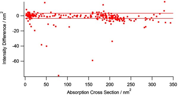
Figure 4 shows the differences between the observed absorbances and those calculated via the catalog method as described in Section 4.1 for the 317 lines that are both in the experimental data and the QM catalog. For the 105 reference lines, these are the same as the residuals of the temperature fit described in Section 3. Since at the line centers, all three approaches provide very similar results, this distribution is representative of the methods described in Sections 4.2 and 4.3 as well and can be considered as a measure of the uncertainty of the results reported here. Large negative differences are likely due to overlapping lines which add intensity at the location of catalog lines rather than to uncertainties associated with the analysis procedures reported here. Inspection of the spectra shows that the two largest positive differences involve blends, but the third largest appears to result from uncertainties in our analysis procedure related to the removal of the baseline.
Figure 4. Intensity difference between the experimentally observed intensity and the catalog intensity for all 317 lines that are included in both. The horizontal lines represent 1% of the intensity of the strongest lines. Large negative differences are in all likelihood due to overlaps with uncataloged lines.
Download figure:
Standard image High-resolution image
5. SUMMARY
This paper reports the complete, variable temperature spectrum of the astrophysical weed ethyl cyanide in the widely observed 210–270 GHz window and the analysis and archiving of these results in astrophysically convenient form. As with the 570–645 GHz region, we find that the QM analyses that form the basis of the usual astrophysical catalogs are massively incomplete at 300 K, primarily due to the difficulty of analyzing perturbed, low-lying vibrational states. We also considered this incompleteness as a function of temperature and found that at 100 K the catalogs would be rather complete with the addition of the interaction states near 200 cm−1, but at temperatures that correspond to recently observed hot cores (500 K) that they would be very incomplete even if the cluster of interacting states near 400 cm−1 were analyzed and included as well. This paper also introduces and validates a spectral synthesis technique that effectively deals with blends and the large data sets that include the spectra of the excited vibrational states, while at the same time being based on data collections in the usual astrophysical catalog format.
We thank the National Science Foundation and JPL/Herschel for their support of this work. This work was also supported by NASA Headquarters under the NASA Earth and Space Science Fellowship Program—Grant NNX09AP10H.