


ABSTRACT
We use the Michelson Doppler Imager and TRACE observations of photospheric magnetic and velocity fields in NOAA 10759 to build a three-dimensional coronal magnetic field model. The most dramatic feature of this active region is the 34° rotation of its leading polarity sunspot over 40 hr. We describe a method for including such rotation in the framework of the Minimum Current Corona model. We apply this method to the buildup of energy and helicity associated with the eruptive flare of 2005 May 13. We find that including the sunspot rotation almost triples the modeled flare energy (1.0 × 1031 erg) and flux rope self-helicity (−7.1 × 1042 Mx2). This makes the results consistent with observations: the energy derived from GOES is 1.0 × 1031 erg, the magnetic cloud helicity from WIND is −5 × 1042 Mx2. Our combined analysis yields the first quantitative picture of the helicity and energy content processed through a flare in an active region with an obviously rotating sunspot and shows that rotation dominates the energy and helicity budget of this event.
Export citation and abstract BibTeX RIS
1. INTRODUCTION
High-quality observations of the slow evolution of photospheric magnetic fields in active regions, in concert with improved models of the gradual storage of coronal energy associated with them, are presently advancing understanding of the physical processes that power solar flares and coronal mass ejections (CMEs) much beyond a qualitative cartoon level. Sunspot rotation was first observed nearly a century (Evershed 1910; St. John 1913). However, accurate measurement of the rate and amount of rotation with high spatial resolution and temporal continuity for long periods of time is a much more recent capability. Brown et al. (2003) studied seven cases of rotating sunspots using white light observations from TRACE (Handy et al. 1999), and found sunspots that rotated as much as 200° over 3–5 days. Comparable values have been found by others (Zhang et al. 2007; Liu et al. 2008). Zhang et al. (2007) studied several rotating spots in NOAA 10930 and found 240° total rotations in periods from two to three days. Liu et al. (2008) studied the super-AR NOAA 10486 and found about 220° over six days.
Stenflo (1969) and Barnes & Sturrock (1972) first suggested that such sunspot rotation may build up energy that is later released in flares. Several authors have found temporal and spatial relationships between rotating sunspots and flares (Brown et al. 2003; Tian & Alexander 2006; Yan & Qu 2007; Yan et al. 2008; Zhang et al. 2008; Tian et al. 2008; Nightingale et al. 2002). However, the temporal relationship is not strong (Zhang et al. 2008), as one would expect if the energy and helicity are stored in the corona, and not promptly released after it passes through the photosphere.
In this work, we focus our attention on the slow coronal energy and helicity storage that is associated with sunspot rotation, and study its magnitude in comparison to all other motions in an active region whose major spot shows strong rotation. Zhang et al. (2008) estimated the five-day helicity transport through the photosphere associated with the rotation of several sunspots in NOAA 10486 using a simple cylindrical approximation. They showed that it was comparable to that derived by local correlation tracking (LCT) of magnetic features in an MDI magnetogram sequence of the whole active region over the same five days. Our work differs from that of Zhang et al. (2008) in one important respect: we explicitly address the issue of the storage of helicity and energy in the corona, through the use of the Minimum Current Corona (MCC; Longcope 1996), a self-consistent, analytical model of the quasi-static evolution of the three-dimensional coronal field due to photospheric motions. We explicitly develop the model to enable our study of the importance of sunspot rotation relative to, for example, braiding motion of magnetic features. The MCC model provides a powerful tool for quantifying the energetic and topological consequences of changes of connectivity by reconnection and subsequently the helicity transfer between magnetic domains.
This slow energy storage is often inferred observationally using the time-rate-of-change of relative helicity flux as a proxy (Berger & Field 1984; van Driel-Gesztelyi et al. 2003). The time-rate-of-change of relative helicity due to photospheric motions is given by a surface integral involving velocity and magnetic field. For brevity, we hereinafter refer to this total integral as the helicity flux, recognizing that there is no spatially resolved density capable of revealing the local distribution of helicity changes (Pariat et al. 2005). The helicity flux integral can be decomposed into a sum of terms corresponding to distinct types of photospheric motion and modes of energy storage. A term involving vertical velocity corresponds to the injection of helicity and energy by emergence of current-carrying flux. Terms involving the horizontal velocity are further separated into braiding and spinning contributions (Welsch & Longcope 2003; Longcope et al. 2007b). The braiding term captures energy and helicity injected as photospheric magnetic features move relative to one another, while the spinning term captures energization when they rotate.
Models have tended to investigate energization most often by emergence or braiding and not by internal spinning. Shearing of an arcade, for example, is a case of pure braiding as the opposite polarities sweep past one another parallel to the polarity inversion line (Klimchuk & Sturrock 1989; Longcope & Beveridge 2007).
We present here the case of a large solar flare in an active region (NOAA 10759) that had for many days undergone no major change other than the rotation of its largest sunspot. The M8.0 eruptive solar flare occurred on 2005 May 13 starting at 16:03 UT during a quiet period of solar activity, in a relatively simple global magnetic configuration. The active region exhibited a sigmoidal structure in ultraviolet, strong Hα emission from two flare ribbons, and a very fast CME (Yurchyshyn et al. 2006; Liu et al. 2007). Jing et al. (2007) carried out a multi-wavelength study to describe the observations with sigmoid-to-arcade transformation. However, no quantitative study has been done to explain energetics of this flare due to sunspot rotation. We are able to quantitatively model the coronal energy storage that would have occurred without the sunspot spinning (i.e., due to braiding alone), as well as that which did occur with the sunspot rotation. Through a comparison, we find that the sunspot rotation alone was responsible for the most of the energy storage, and furthermore, that the energy stored is consistent with that released by the subsequent large flare.
Our work builds on the analysis of Longcope et al. (2007a, Paper I), which constructed the first quantitative model of flux and helicity processed through three-dimensional reconnection in a two-ribbon flare and CME. Longcope et al. (2007a) used the MCC model to study the energetics and topology of the X2 flare of 2004 November 7. They partitioned a magnetogram sequence to create a model of the evolving photospheric magnetic field as moving discrete flux sources, computed the evolving coronal magnetic field, and applied the MCC model to estimate the stored energy and helicity. They found that the amount of flux that would need to be reconnected during the flare in order to release the stored energy compared favorably with the flux swept up by the flare ribbons measured using TRACE 1600 Å images. They showed that the amount of stored energy predicted by the model was comparable to that released by the observed X-ray flare. However, the flux rope associated with this event was observed to contain at least 4 times more magnetic helicity than the model prediction.
Because the active region hosting the flare/CME event of 2004 November 7 (from Paper I) showed no obvious sunspot rotation, the authors anticipated that the analysis using the MCC model and the representation of each magnetic feature by a single point magnetic charge needed only to account for the braiding motion of those charges. In the present paper, we further develop the method used in Paper I, examining the M8.0 flare/CME event on 2005 May 13, whose preflare magnetogram sequence was different in an important respect—obvious sunspot rotation was present. We describe how we included rotation into the model using a quadrupolar representation of the rotating sunspot, rather than a unipolar one. On the basis of the MCC model and the quadrupolar representation, we calculate the amount of flux, energy, and helicity transferred by reconnection and compare these quantities for rotating and non-rotating cases. We find that the rotation of the large positive sunspot produces 3 times more energy and magnetic helicity than the non-rotating case, and our inclusion of sunspot rotation in the analysis brings the model into substantial agreement with observations.
The paper is organized as follows. In Section 2, we present the magnetogram data used in the study. In Section 3, we discuss the helicity injected by the photospheric motions derived from the MDI magnetograms, describe rotation of the large positive sunspot observed with TRACE and the way we incorporate it in our model. In Section 4, we calculate the reconnection flux from the model and compare it with the measured flux from the flare observations. Section 5 lists properties of the separators found in the coronal topology at the time of the flare. In Section 6, we compare results in two cases: rotating and non-rotating. Finally, we summarize our results in Section 7.
2. PARTITIONING OF THE MAGNETOGRAM SEQUENCE
For the topological analysis that follows we partition the observed photospheric magnetic field into a set of persistent unipolar regions (Barnes et al. 2005; Longcope et al. 2007b). Our magnetic field data consist of a sequence of 25 low-resolution Solar and Heliospheric Observatory/The Michelson Doppler Imager (SOHO/MDI) magnetograms (2'' resolution, level 1.8, Scherrer et al. 1995) obtained at 96 minute intervals over a 40 hr period beginning at t0= May 11 23:59 UT and ending at tflare= May 13 16:03 UT, near the start time of the flare. We correct each individual pixel of each magnetogram for the viewing angle assuming the photospheric field to be purely radial. The basic step in partitioning is grouping pixels exceeding a threshold Bthr = 35 Gauss downhill from each local maximum into individual partitions. We then combine partitions by eliminating any boundary whose saddle point is less than 300 Gauss below either maximum it separates. Finally, we discard any partitions with less than 7.6 × 10¹⁹ Mx of net flux on the premise that they are too small to contribute significant energy to the active region magnetic field. As a result, approximately 84% of the flux in each polarity is assigned to one of 48 different partitions.
Each partition is assigned a unique label, which it maintains throughout the sequence. To accomplish this, we derive a local correlation tracking (LCT) velocity (November & Simon 1988) from all successive pairs of magnetograms in the sequence. To prevent spurious effects from noise, we correlate only pixels with magnetic field strength over 45 Gauss. We use a Gaussian apodizing window of 7'', generate a reference partitioning by advecting the previous partitions to the present time using LCT velocity pattern, and assign a partition the label of the reference partition which it most overlaps. We find that performing the process in reverse chronological order back from the flare time provides the most stable partitioning.
Applying these procedures to the magnetogram sequence results in a set of evolving unipolar partitions. In Figure 1, we show the spatial distribution of these partitions in the magnetogram nearest to the flare time, on 2005 May 13 16:03 UT. The largest positive partition, P01, has flux 1.1 × 10²² Mx, which is more than half of the total positive flux (2.0 × 10²² Mx); negative flux is not similarly concentrated in any one dominant partition.

Figure 1. Partitions are determined for NOAA 10759 on May 13 16:03 UT, near the start time of the flare, see Section 2. The gray scale magnetogram shows the radial magnetic field Bz(x, y) scaled from −1000 G to 1000 G. The partitions are outlined and the centroids are denoted by +'s and x's (positive and negative respectively). To account for rotation, we divide P01 into three sources of equal flux which rotate with angular velocity inferred from TRACE white light data, as described in Section 3.4. Axes are labeled in arcseconds from disk center.
Download figure:
Standard image High-resolution imageThe methods of calculation of energy and helicity buildup that we use in this paper, following Paper I, do not accommodate flux emergence or cancelation. By assumption all changes in coronal connectivity in the calculation are due to translational centroid motion. We thus form what we call the reduced model of the partitions, in which all individual partition fluxes are held strictly constant and equal to the fluxes at the time of the flare (tflare = May 13 16:03 UT). During the 40 hr covered by the magnetogram sequence the total flux of the active region in the actual observations remains almost constant—the total positive (negative) magnetic flux is  (−2.2 × 10²² Mx) at t0 and
  (−2.1 × 10²² Mx) at tflare. Hence the reduced model is not unrealistic in the present study.
The MDI observations exhibit magnetic field saturation inside P01, which lowers its total flux. To estimate the importance of this saturation, we identify the saturated area with an outer contour of 1800 G. If we arbitrarily fill the saturated area with pixels of 2200 G field strength (a plausible value), then it changes the flux of P01 by only 2%. We therefore ignore this saturation effect.
We now represent each magnetic partition  resulting from the partitioning process as a magnetic point charge (or magnetic point source) described by the coordinates of its centroid (
 ) and its magnetic flux (Φa)
Since our objective is to calculate changes in connectivity due to proper motion of the charges, we project the centroid location of each point charge from the image plane onto a plane tangent to the solar surface. We compensate for rotation by fixing the plane's point of tangency, also the coordinate origin, to a point on the solar surface rotating at a given latitude-dependent speed (Howard et al. 1984).
Ideally, each partition tracks a particular photospheric flux cell from one frame to another. If we discard emergence or submergence, the net flux of a "good" partition  should be conserved (dΦa/dt = 0), and the velocity of its centroid
  should match the flux-weighted LCT velocity
where u(x, y) is the horizontal photospheric velocity field from local correlation tracking, and  is the centroid position defined in Equation (1). If there is some vertical flow vz across the photosphere in addition to a horizontal component vh, then u becomes "flux transport velocity": u = vh − (vz/Bz)Bh (Démoulin & Berger 2003).
3. SPIN HELICITY
3.1. Basic Definition
From the vertical magnetic field Bz(x, y) and the horizontal velocity field u(x, y) (found from the LCT, for example) the time rate of change of relative helicity, i.e., helicity flux is given by the surface integral
where AP is the vector potential, required to be divergence-free through the corona and tangent to the photosphere, which generates the potential field matching the photospheric normal field, Bz, (see Equation (10) in Longcope et al. 2007b).
We may decompose the full vector potential AP into a sum of contributions from each magnetogram partition by restricting the region of integration. Then expression (Equation 3) becomes
The first term is a sum of spin helicity fluxes from individual partitions, denoted  , and the second term is the exact braiding helicity flux,
  (Welsch & Longcope 2003; Longcope et al. 2007b). The vector potential AaP generates a potential field whose normal matches Bz within
  and Bz = 0 everywhere outside
  ; it is subject to the same conditions as AP.
The definition of a spin helicity flux for a single partition seems at odds with the inherent non-localizability of helicity flux. It was shown by Pariat et al. (2005) that the helicity flux integral cannot be meaningfully restricted to any portion of the photosphere in order to deduce where helicity is coming from. The spin helicity flux is not, however, a simple restriction of the helicity flux integral since it contains the vector potential AaP rather than AP. In fact, the spin helicity,  , can be interpreted as the difference between total helicity fluxes, integrated over the entire photosphere, from two velocity fields u and v differing only within
  . The first, u, is the actual velocity field, including any spinning motion internal to
  . The second, v, is identical to u everywhere except in
  . Even there it produces the same field evolution

but the total spinning motions over the partition  cancel, by which we mean
Subtracting the total helicity fluxes generated by these two velocity fields, we obtain
In the second term on the right-hand side of Equation (7) ∇ × AbP = Bbz = 0, hence AbP = ∇χb. Then after integration by parts and using  and Equation (5) the second and the third terms of Equation (8) become zero. The result is an integral over
  alone, equal to the term
  .
.
The above decomposition appears similar to a decomposition of the total helicity integral into self-helicity and mutual helicity3 based on a subdivision of the coronal volume into subvolumes (Longcope & Malanushenko 2008). Even if the coronal subvolumes are based on the photospheric partitions, they will generally subdivide partitions according to coronal field connectivity. There will therefore usually be different numbers of coronal subvolumes to which self-helicities are assigned than partitions to which spin helicities are assigned. Furthermore, the self-helicity, or its time-rate-of-change, depends on coronal interconnection between partitions (Pariat et al. 2005). These discrepancies make it clear that the time-rate-of-change of a self-helicity does not correspond to any spin helicity flux; the two decompositions are not directly related. For that matter the spin helicity flux attributed to one particular region cannot be equated with helicity injected into field lines connected to that region alone. Instead it is the helicity which would not have been injected had the internal motion within that particular region been different (i.e., satisfied Equation (6)).
3.2. Spin Helicity from LCT Using the MDI Data
In our calculations, instead of the exact expression for the braiding helicity flux, we use a simplified version, denoted  , in which the integrals are expanded in powers of the separation between partitions
  and
and  :
:
When the active region is at the disk center, we may calculate helicity through the plane of the sky as observed. However, when the active region is far from the disk center the projection effects are important. Hence, we compute the relative helicity flux through the tangent plane.
For the NOAA 10759, we apply LCT to the 40 hr magnetogram sequence before the flare to find the flow field u. Using this flow field in Equation (3) and integrating over the entire sequence gives a net change in total relative helicity ΔHLCT = −6.1 × 1042 Mx2. Using the flow field, along with the partitions, in Equation (4) gives a spin helicity ΔHLCT, sp = −2 × 1042 Mx2. From Equation (10) the simplified braiding helicity is  . Their sum is
  . The discrepancy between ΔHLCT and
  is caused by approximating the braiding helicity contribution by the motions of the region centroids as described in Equation (10):
  .
.
Since the spin helicity flux is proportional to the magnetic flux squared and P01 dominates the magnetic flux of the active region, the spin helicity fluxes from other partitions are negligible compared with that from P01. The spin helicity flux of P01 alone,  , found from the LCT can be used to compute an effective rotation rate (pluses in Figure 2):
Figure 2. Top: GOES light curve. Bottom: Evolution of the rotation rate of P01 inferred from; diamonds—TRACE WL observations, plus signs—LCT velocity field. Dotted lines indicate the start and the end of the magnetogram sequence (left, May 11 23:59 UT; right, May 13 16:03 UT), see Section 3.
Download figure:
Standard image High-resolution image
where Φ is the magnetic flux of P01 (Longcope et al. 2007b).
We show in the following section that the resolution of the MDI observations (96 minutes, 2'' pixels, 7'' apodizing window) covering the flare in NOAA 10759 is insufficient to accurately measure the rotation rate within the large sunspot P01. This failure is consistent with Longcope et al. (2007b), who showed that the rotation rate scales inversely with the LCT apodizing window and is twice as high from the high-resolution MDI data (0 6 pixels) as from the low-resolution data (2'' pixels) for a 1-hr magnetogram cadence. To obtain a measurement of the rotation rate more accurate than possible from our low-resolution 96 minute MDI data, we use TRACE white light (WL) observations of P01. Since this single rotation is expected to dominate the overall spin helicity, we forego improved measurements for any other region.
3.3. Spin Helicity from TRACE White Light Data
Observations in NOAA 10759 of the large, leading sunspot in TRACE white light images show it to be rotating around its umbral center during 2005 May 11–16 at about 14° N solar latitude. From previous measurements of rotating sunspots observed in the high-resolution TRACE WL data (Brown et al. 2003), the rotation speeds may vary from about 0 5 to 3° hr−1, mostly counter-clockwise (CCW) in the northern solar hemisphere and clockwise (CW) in the southern hemisphere for solar cycle 23. We have developed a single-slice procedure used previously in Tian et al. (2008) to measure the rotation speeds of sunspots observed by TRACE. It is less complex than the computer-intensive image comparison method of Brown et al. (2003). The procedure utilizes some of the slice tools in the ANA Browser (Hurlburt et al. 1997), which can be found online as part of SolarSoft (SSW; Freeland & Handy 1998). We have the browser select TRACE WL images with a 10 minute cadence over a 6 hr interval and overlay and align them to best remove the effects of solar rotation. A circle slice is generated, using the browser tools, whose radius is located from the center of the umbra to about one-third of the way into the penumbra from the umbral-penumbral interface. The latter position is approximately where the maximum rotation speed along the radius was found in Brown et al. (2003). Circle slices of the temporal set of overlaid images are then combined into a time–distance plot for the image set, from which a diagonal linear feature is selected, providing the rotation speed and the direction of rotation, if any, for that 6 hr interval. Typically, only one feature can be identified (i.e., see Figure 7 in Brown et al. 2003).
Of course other methods and other data sets could be used, i.e., MDI magnetic field measurements. However, TRACE WL observations have three important advantages. First, the TRACE observing cadence is much higher (10 minutes versus 96 minutes). Second, the TRACE WL spatial resolution is higher (1'' versus 2''). Finally, the TRACE WL observations have much more structure resolved in the penumbra.
In Figure 2, we compare the rotation rate of P01 during 40 hr inferred from the TRACE WL observations (diamonds) with the rotation rate of P01 inferred from the MDI observations (pluses, see Equation (11)). The diamonds are the average of two successive measurements. The vertical bars indicate the range of those two measurements which may reflect two different fittings of the linear feature (see Figure 7 in Brown et al. (2003)). From the plot, we see that our LCT analysis found a rotation rate 4–10 times smaller than the TRACE rotation rate (01–02 hr−1 from MDI versus 08–10 hr−1 from TRACE WL). In fact, it is only 01 hr larger than the rotation rate of the whole active region. We suspect that the observational limitations like low cadence and low spatial resolution along with the large apodizing window compromise the MDI rotation measurement. Independently of the observational limitations, it has been demonstrated that the LCT method intrinsically fails to measure any motion parallel to the isolevels of the distribution of the magnetic field (Gibson et al. 2004) and hence cannot determine the velocity field of an axisymmetric rotating sunspot (P01). Hence we use the average TRACE WL value of the rotation rate of 085 hr−1 (34° in 40 hr).
3.4. Including Spin Helicity in MCC Models
To calculate the energy that can be released by the flare we use the Minimum Current Corona model (MCC; Longcope 1996). This model characterizes the coronal field purely in terms of how it interconnects photospheric source regions. The total flux, interconnecting regions  and
and  , called a domain flux ψa/b, could be computed from the partitioned magnetogram alone. Replacing each unipolar flux region with a single point charge, as we choose to do, results in values of ψa/b only slightly different (Longcope et al. 2009). As the regions or charges move they would be interconnected by different amounts of flux, ψ(v)a/b(t), had the coronal field remained potential. The MCC finds the minimum energy of a field which does not change those connectivities—it constrains the domain fluxes.
Constraining as it does the interconnections between moving sources, MCC is capable of capturing braiding helicity flux into the field. The braiding helicity flux of the moving point sources,  , is given by Equation (10), where
  and
and  are the position and velocity of charge a. The MCC does not, however, constrain the internal anchoring of field lines within a region or source, and therefore cannot constrain spin helicity flux into the field. The unconstrained footpoints are free to execute internal spinning motions in response to evolution, so the spin helicity is not in general zero (Longcope & Magara 2004). On the other hand, the MCC provides no control over what value the spin helicity flux of a given region actually assumes.
In the present case, the major source of helicity flux, and possibly of energy storage, is the spin helicity flux from region P01. In order to accurately model, the energy storage due to this purely internal motion (internal to the region defined by our partitioning) using MCC we must modify the photospheric model. Rather than constraining connection to P01 as a whole, we represent that partition with three separate point sources, P01a, P01b, and P01c, and constrain connections to each one separately. This approach, dubbed a hierarchical model by Beveridge & Longcope (2006), introduces more constraints thereby naturally raising the value of the constrained minimum energy. More significantly, it permits the triad of point charges to be moved relative to one another to create braiding helicity flux beyond what the single-charge model would yield. This "internal" braiding helicity flux can be controlled in order to reproduce the observed spin helicity flux from the same region.
Partition P01 is represented by three equal point sources located about the ellipse so as to match the first three multipole moments of the magnetogram (see Figure 3). The process for doing this, the so-called quadruple method, is described in Appendix A. The original braiding helicity flux,  , will contain a number of terms where P01 is paired with other sources, a. Each such term will be replaced, in the quadrupole model, by three terms pairing a with P01a, P01b, and P01c in turn. The sum of these three terms will approximate the original one as long as the linear dimension of partition P01 is small compared to the separation between P01 and xa. The modified braiding helicity flux will also include six new terms which we collectively designate
where i and j take on values P01a, P01b, and P01c, and  is the rotation rate of the separation vector
  (Berger & Field 1984). To represent the rotation of P01, the three sources P01a, P01b, and P01c are moved about the ellipse by varying the free parameter ζ so as to inject the helicity into P01 at the desired rate
where  is a rate of change of the average angle between the charge pairs (see Figure 3 and Equation (A10) in Appendix A). From here and Equation (11)
where ωP01 is the angular rotation rate of P01 given by TRACE WL observations. This modification allows the quadrupole representation to introduce a form of internal braiding by which we may control spin helicity.
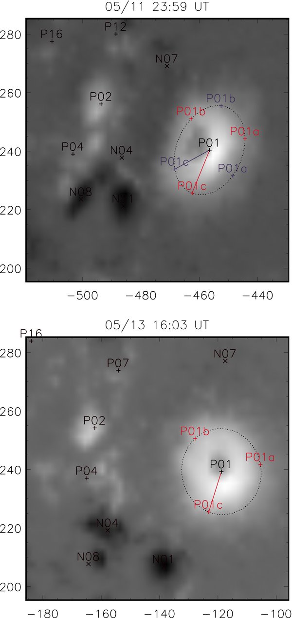
Figure 3. Representation of the rotation of P01 using three poles on an ellipse (dotted curve). Top: Fitted ellipse 40 hr prior to the flare. Bottom: fitted ellipse at the flare time. Blue: 40 hr prior to the flare. Red: flare time. The 34° rotation angle inferred from TRACE WL is used for the value of ψ. Axes are labeled in arcseconds from disk center.
Download figure:
Standard image High-resolution imageThe importance of the P01 spinning as a source of helicity injection is demonstrated by comparing braiding helicity flux of the whole active region from two different quadrupole models. In the first P01a, P01b, and P01c move so as to reproduce the spin helicity flux computed from MDI LCT (01 hr−1, pluses on the Figure 2), while in the second they reproduce the spin helicity flux derived from TRACE WL (085 hr−1, diamonds on the Figure 2). The time-integrated braiding helicity fluxes of the whole active region in the two different cases are

Evidently, rapid motion of the three poles of P01 relative to the other poles injects almost 3 times more helicity than the case where three poles move more slowly. Clearly for meaningful helicity calculations, we must take rotation into account.
4. DOMAIN FLUX CHANGE, ENERGY RELEASE, AND RECONNECTION
We now use our quadrupolar photospheric model (only P01 is represented by a charge triad) to model the energy buildup prior to the flare. To apply the model, we compute connectivities, ψ(v)a/b, from potential fields before and after the energy buildup: t0= May 11 23:59 UT and tflare= May 13 16:03 UT. To calculate the domain fluxes, ψ(v)a/b, at either time, we use a Monte Carlo method (see Barnes et al. 2005) wherein field lines are initiated from point charges in random directions and followed to their opposite end.
Values of ψ(v)a/b from the magnetogram sequence, ψ(v)a/b(t0= May 11 23:59 UT), ψ(v)a/b(tflare= May 13 16:03 UT), and their difference, Δψ(v)a/b = ψ(v)a/b(tflare) − ψ(v)a/b(t0), are listed in each cell of Table 1 where a (b) are positive (negative) sources listed in the first column (row), and t refers to the time dependence that arises from the point source motions during the sequence. Domains with Δψ(v)a/b>0 (Δψ(v)a/b < 0) gain (lose) domain flux due to magnetic charge motions. In Figure 4, dotted paths show the motions of each point charge during the preflare magnetogram sequence. Straight solid and dashed lines connect poles whose domains exhibit the larger changes in domain flux, i.e., changes above 0.23 × 10²¹ Mx.

Figure 4. Motions and important connections of the labeled poles in the preflare magnetogram sequence, see Section 4. The dotted curves show the paths taken by the poles in forty hours in the co-rotating plane from May 11 11:58 to May 13 16:03 UT, ending at the corresponding pole labels, which show positions on May 13 16:03 UT. The paths of P01a,b,c clearly show the CCW rotation of this spot. The solid (dashed) lines connect each pole pair whose potential-field domain flux ψ(v)a/b has increased (decreased) by more than 0.23 × 10²¹ Mx in forty hours between May 11 11:58 UT sand May 13 16:03 UT: |Δψ(v)a/b|>0.23 × 1021 Mx (see Table 1).
Download figure:
Standard image High-resolution imageTable 1. Domain Fluxes ψ(v)a/b and their Changes Δψ(v)a/b from Selected Point Sources as Described in Section 4; All Values are in Units of 1021 Mx
| Source | N01 | N02 | N03 | N04 | N05 | N06 | N08 | N10 | Φa | dP | dN |
|---|---|---|---|---|---|---|---|---|---|---|---|
| P01a | ⋅⋅⋅ | 0.2 − 0.20.0 | 0.0 + 0.30.3 | ⋅⋅⋅ | ⋅⋅⋅ | 1.1 − 0.01.1 | ⋅⋅⋅ | ⋅⋅⋅ | 3.6 | 0.3 | −0.3 |
| P01b | ⋅⋅⋅ | 0.0 + 0.70.7 | 1.7 + 0.11.8 | 0.0 + 0.20.2 | 0.5 − 0.30.3 | 0.7 − 0.10.6 | 0.0 + 0.00.0 | ⋅⋅⋅ | 3.6 | 1.1 | −0.4 |
| P01c | 0.9 − 0.10.9 | 1.3 − 0.70.6 | 0.2 − 0.20.0 | 0.7 − 0.20.4 | 0.0 − 0.00.0 | 0.3 + 0.20.5 | 0.1 + 0.20.4 | ⋅⋅⋅ | 3.6 | 0.4 | −1.2 |
| P02 | ⋅⋅⋅ | 0.3 + 0.40.6 | 0.5 − 0.20.3 | 0.2 − 0.20.0 | 0.0 − 0.00.0 | 0.0 + 0.00.0 | 0.0 − 0.00.0 | 0.5 − 0.10.4 | 1.4 | 0.4 | −0.4 |
| P03 | 0.0 + 0.10.1 | 0.3 − 0.20.0 | ⋅⋅⋅ | ⋅⋅⋅ | ⋅⋅⋅ | 0.0 + 0.00.0 | 0.0 + 0.00.1 | ⋅⋅⋅ | 1.6 | 0.1 | −0.2 |
| P04 | ⋅⋅⋅ | 0.7 + 0.10.9 | ⋅⋅⋅ | 0.1 + 0.20.2 | ⋅⋅⋅ | ⋅⋅⋅ | 0.3 − 0.20.0 | 0.1 − 0.10.0 | 1.1 | 0.3 | −0.3 |
| P07 | ⋅⋅⋅ | ⋅⋅⋅ | 0.0 + 0.00.0 | ⋅⋅⋅ | 0.0 + 0.20.2 | 0.0 − 0.00.0 | ⋅⋅⋅ | 0.0 + 0.10.1 | 0.2 | 0.3 | −0.0 |
| P12 | ⋅⋅⋅ | ⋅⋅⋅ | 0.1 − 0.10.0 | ⋅⋅⋅ | 0.4 + 0.10.5 | ⋅⋅⋅ | ⋅⋅⋅ | 0.0 + 0.00.0 | 0.5 | 0.1 | −0.1 |
| P16 | ⋅⋅⋅ | ⋅⋅⋅ | 0.2 − 0.20.0 | ⋅⋅⋅ | 0.1 + 0.20.3 | ⋅⋅⋅ | ⋅⋅⋅ | 0.0 + 0.00.0 | 0.3 | 0.2 | −0.2 |
| Φb | 1.0 | 2.9 | 2.6 | 0.9 | 1.3 | 2.5 | 0.5 | 0.5 | |||
| dP | 0.1 | 1.2 | 0.5 | 0.4 | 0.5 | 0.3 | 0.3 | 0.1 | 3.2 | ||
| dN | −0.1 | −1.2 | −0.7 | −0.4 | −0.3 | −0.2 | −0.2 | −0.1 | −3.1 | ||
Notes. Each row or column is one of the largest positive or negative sources. Each entry gives the fluxes at May 11 23:59 UT (upper left) and May 13 16:03 UT (lower right) and the net change (center); a dash indicates that no connection exists between those sources. The two far right columns (bottom rows), dP and dN, give sum of all negative (flux excess) and all positive (flux deficit) numbers in the row (column). Φa and Φb give the total source flux of that region. These are greater than the sums across the rows or columns due to the contributions of omitted sources.
Download table as: ASCIITypeset image
Under the assumption that no reconnection occurs during the 40 hr of the magnetogram sequence, the domain fluxes could not have changed, and the field could not have remained in a potential state. In this way, the lack of reconnection leads to a storage of free magnetic energy, energy above that of the potential field, which could then be released by reconnection. To achieve the maximum energy release, the field inside the flaring domains would need to relax to its potential state. In other words, reconnection will need to transfer flux from flaring domains for which Δψ(v)a/b < 0 and into flaring domains for which Δψ(v)a/b>0. Our working hypothesis is that the transfer of this flux through reconnection was responsible for the M8.0 flare beginning at tflare= May 13 16:03 UT. In the following section, we first use observations by TRACE to identify the flaring domains, and then we measure the reconnection flux for those domains.
4.1. Model Reconnection Flux from Connectivity Matrix
A topological skeleton describes the topology of the magnetic field in the photosphere and corona. Several features are relevant to the present discussion (Gorbachev et al. 1988, 1989; Mandrini et al. 1991, 1993; Démoulin et al. 1993, 1994; Bagalá et al. 1995; Priest et al. 1997; Longcope & Cowley 1996; Longcope 2005). A null is a point where all three components of the magnetic field vanish—for example, a point between two point charges of the same polarity. A spine is a line between two such charges, connecting them through their associated null. In a typical two-ribbon flare geometry, the ribbons lie along the photospheric projections of spine lines to within the accuracy of the point-charge representation of the magnetic field. A separatrix surface is a boundary between different domains. A separator is a line in three dimension where two separatrix surfaces intersect, at which reconnection can take place.
We have computed the topological skeleton at the end time of the preflare magnetogram sequence, immediately before the flare. A superposition of the spine lines from this skeleton onto a TRACE 1600 Å flare ribbon image is shown in Figure 5. This overlay of TRACE ribbons gives an indication of which domains are involved in the flare. The overlay suggests that the eastern ribbon is associated with the spine connecting null points A01, A02, A03, A04, A05, A06, A07, and A08, and the western ribbon with the spine connecting B09, B10, B11, B12, and B13. The largest negative poles adjacent to those nulls are N18, N05, N10, N03, N06, N02, N08, N04, and N01. The largest positive poles are P03, P01c, P01a, P01b, P02, and P04. The total magnetic flux in these polarities is well balanced: −1.3 × 10²² Mx versus 1.5 × 10²² Mx. The identification of these poles helps to determine the flaring domains.

Figure 5. TRACE 1600 Å image, plotted as reverse gray scale, with elements of the topological skeleton superimposed. The skeleton calculated for 16:03 is projected onto the sky after its tangent plane has been rotated to the time of the TRACE observations (16:52 UT). Positive and negative sources are indicated by +'s and x's, respectively. The triangles represent the labeled null points. The curved line segments show spine lines associated with the reconnecting domains, as discussed in Section 4.1. Axes are in arcseconds from disk center.
Download figure:
Standard image High-resolution imageTable 1 lists the domain flux measurements associated with these poles. The pre-reconnection domain flux of the actual field is the one at the beginning of the stressing: ψa/b = ψ(v)a/b(0), on the assumption that the field began in a potential state at 2005 May 11 23:59 UT. The difference between connectivities of the present potential field and the actual field value is quantified by
since ψa/b = ψ(v)a/b(t0).
Domains with excess flux (relative to the potential field) are those with Δψa/b>0; these have negative values in Table 1. Domains with deficit flux are those with Δψa/b < 0. The total flux excess (deficit) of all ribbon domains, ΔΨ↓ (ΔΨ↑), can be found by summing all the negative (positive) domain flux changes in the Table 1. These give two estimates for the net flux transfer which must occur in the two-ribbon flare: ΔΨ↓ = 2.8 × 10²¹ Mx, ΔΨ↑ = 2.7 × 10²¹ Mx (within the flaring domains connecting sources on the ribbon N18, N05, N10, N03, N06, N02, N08, N04, and N01 and P03, P01c, P01a, P01b, P02, and P04). The arrows indicate how the fluxes will change under reconnection: those with an excess will decrease, while those with a deficit will increase. Were it not for connections outside the ribbon set with external sources, these two quantities would exactly match, since one domain's increase comes from another domain's decrease: ΔΨ↓ = 3.1 × 10²¹ Mx, ΔΨ↑ = 3.2 × 10²¹ Mx (adding external sources P16, P12, P07, see Table 1).
4.2. Observed Reconnection Flux from Ribbon Motion
The model reconnection flux discussed in the previous section could be compared with measured reconnection flux from the ribbon observations. The M8.0 flare was observed by TRACE at 1600 Å with 20–30 s cadence between 16:00 UT and 20:20 UT. The two flare ribbons became visible in 1600 Å images at 16:27 UT and peaked at 16:57 UT. To measure the total reconnection flux, we count all pixels that brightened during any period of the flare and then integrate the signed magnetic flux encompassed by the entire area (Qiu et al. 2007). According to the standard atmosphere model of Vernazza et al. (1981), we choose h = 2000 km as the presumed formation height of the ribbons in the chromosphere. We extrapolate the MDI photospheric magnetogram to the height of 2000 km using a potential field extrapolation algorithm. This correction reduces the value of the observational reconnection flux by approximately 20% (Qiu et al. 2007).
The total measured reconnection fluxes at 17:02 UT, when the reconnection flux rate is close to zero, amount to Ψ+ = (4.1 ± 0.4) × 1021 Mx, and Ψ− = (4.0 ± 0.4) × 1021 Mx for positive and negative fluxes respectively (for h = 2000 km, the ribbon-edge cutoff is taken to be 10 times the background intensity). The uncertainties come from estimates of the mis-alignment between the MDI and TRACE data, ribbon edge identification and inclusion of transient non-ribbon features with the ribbon areas. The modeled reconnection flux we gave in Section 4.1 (ΔΨ↑ = 2.8 × 10²¹ Mx) compares favorably with that derived from TRACE (Ψ+ = (4.1 ± 0.4) × 1021 Mx).
As an aside, we consider how much of the flux in the ribbon poles is reconnected during the flare. The modeled reconnection flux ΔΨ↓ = 3.1 × 10²¹ Mx is only a fraction of the total flux in all of the source regions on the ribbon (1.5 × 10²² Mx, − 1.3 × 10²² Mx). It means that only one-fourth (3.1/13 ≈ 1/4) of the field anchored to these source regions has been stressed to the point that reconnection would be energetically favorable.
5. FLARE ENERGY AND FLUX ROPE HELICITY
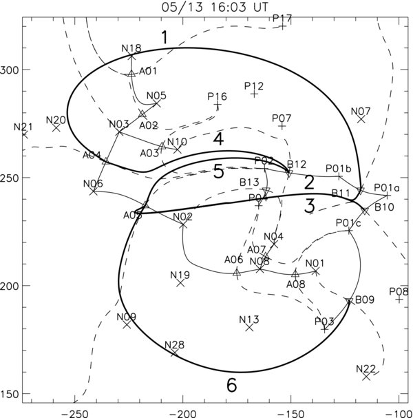
We apply the MCC (as described in Appendix B) to the quadrupolar model where rotation rate is determined from the TRACE observations. This produces an estimate of the energy and helicity available for the flare. From the 19 separators, which link the 13 null points lying on the ribbon, we chose six most energetic flaring separators with separator flux larger than 2 × 10²⁰ Mx. Figure 6 shows the structure of the topological skeleton with these six separators (bold). Table 2 lists their index (i, same as in Figure 6), nulls they connect (nulls), length (Li), maximum height (zi,max ), flux (Δψi), current (Ii), energy ( ) and helicity (Hi). We group six separators into two groups according to the nulls they connect. The first group, internal to the P01 flux system (1, 2, 3), contains one of the nulls whose spines connect to components of P01: B10 or B11. The second group, external to the P01 flux system (4, 5, 6), connects the nulls lying outside P01. Table 2 indicates that the most energetic separator (i = 3) connecting A05–B10 (4.6 × 1030 erg) has the largest separator flux Δψi = −0.68 × 10²¹ Mx. It connects two nulls: A05 which lies between N02 and N06 and B10 which lies between P01c and P01a. In the bottom row of Table 2, total energy (
 ) and helicity (H) are given. The net helicity of all contributions H ≃ −1.4 × 1043 Mx2 accounts for most of the helicity injected by the motions of the model flux sources, shown in Figure 4. The absolute value of the net helicity including the other 13 separators is slightly smaller (H ≃ −1.3 × 1043 Mx2) as there are some separators lying far from the PIL which contain positive helicity. The difference between the net helicity calculated from LCT and MCC provides a measure of the uncertainty of the MCC model. The total energy is
  erg.
erg.
Figure 6. Elements of the topological skeleton footprint on May 13 16:03 UT, plotted on the tangent plane, see Section 5. Thin solid lines are the spine curves and dashed lines are the photospheric footprints of separatrices. Thick solid lines are flaring separators. The large numbers near each separator are the separator indices i, as in Table 2. Axes are in arcseconds from disk center.
Download figure:
Standard image High-resolution image
Table 2. Properties of the Flaring Separators, Rotating Case
| i | Nulls | Li | zi,max | Δψi | Ii |  |
Hi | |
|---|---|---|---|---|---|---|---|---|
| − | + | (Mm) | (Mm) | (1021 Mx) | (GA) | (1030 erg) | (1042 Mx2) | |
| 1 | A04 | B11 | 232.7 | 87.1 | −0.49 | −55.6 | 1.19 | −2.91 |
| 2 | A05 | B11 | 134.3 | 45.0 | −0.45 | −93.3 | 1.81 | −2.93 |
| 3 | A05 | B10 | 135.1 | 45.0 | −0.68 | −164.6 | 4.65 | −5.18 |
| 4 | A04 | B12 | 84.2 | 22.6 | −0.25 | −65.7 | 0.74 | −0.99 |
| 5 | A05 | B12 | 73.5 | 22.2 | −0.21 | −56.3 | 0.53 | −0.79 |
| 6 | A05 | B09 | 181.0 | 44.3 | −0.46 | −62.3 | 1.24 | −1.43 |
| Total | 10.16 | −14.23 | ||||||
Notes. Separators are listed by their index by i shown in Figure 6. Listed are the names of the nulls linked by the separator, the length Li, and maximum altitude zi,max , of the separator in the potential field at May 13 16:03 UT. The flux discrepancy, Δψi, between that field and the initial one (May 11 23:59 UT), leads to the current Ii, which in turn leads to self-free-energy  and helicity Hi on each separator. The quantities Δψi, Ii,
  and Hi are described in Appendix B.
Download table as: ASCIITypeset image
We may test the model by comparing these energy and helicity values to observations. The total energy of the flare can be estimated from the GOES observations. Using GOES analysis software in SolarSoft, the ratio of the two channels (1–8 Å and 0.5–4 Å) may be compared to the response functions of the GOES instrument to estimate the plasma temperature (Thomas et al. 1985) during the interval of elevated X-ray flux. Based on a synthetic solar spectrum, these temperatures provide the total emission measure. Integrating over the entire spectrum and over the interval of the elevated X-ray flux gives a total radiated energy of 1.0 × 1031 erg. This energy value agrees favorably with the model value  erg. However, the almost exact agreement is certainly fortuitous since there are many uncertainties involved in the energy calculations. First, the model used in GOES is quite simplistic: it assumes a fully filled isothermal plasma. Second, the MCC model provides lower bound on the stored energy since it assumes the ideal quasi-static evolution. Finally, there are uncertainties in the measurements of the rotation rate from TRACE.
An interplanetary coronal mass ejection (ICME) was observed near Earth on 2005 May 15. From in situ magnetic field observations with Wind spacecraft, it has been found that the interplanetary structure is formed by two close consecutive magnetic clouds (Dasso et al. 2009). One of the magnetic clouds is linked to the M8.0 event studied here. Using the Grad–Shafranov method, the self-helicity of this magnetic cloud is HMC = −5 × 1042 Mx2 (Qiu et al. 2007). If half of the total mutual helicity from the MCC model (see Table 2) ends up as self-helicity of the flux rope created by reconnection, then the ejected flux rope would carry  , which compares favorably with the observed value.
The calculations above are given for the case where the quadrupolar representation of region P01 is rotated at the rate determined from TRACE WL observations: 0.85° hr−1 (34° in 40 hr). The uncertainty of 013 or 15% in the average rotation rate leads to uncertainties of the model reconnection flux, energy and helicity given above: 23% in the largest separator flux ψ, 18% in the total helicity H, 29% in the total energy  and 6% in the total reconnection flux ΔΨ.
6. THE IMPORTANCE OF ROTATION
In this work, we have introduced a method for taking into account the rotation of magnetic partitions in the framework of a minimum current corona (MCC) model. Applying the MCC model to NOAA 10759, and accounting for the observed rotation of its leading spot, we have calculated the energy and helicity available to the flare and eruption of 2005 May 13. We have seen that the use of this method yields estimates of energy and helicity that compare favorably with observations of eruptive flare.
We now seek to understand the role of played by sunspot rotation alone by comparing the rotating case, where three poles representing P01 rotate uniformly at a rate of 085 hr−1 for the 40 hr of the magnetogram sequence, with the non-rotating case, where the three poles P01a-c are kept at the same angle  (see Appendix A) as in the magnetogram at tflare throughout the 40 hr buildup. These charges do move in order to account for the motion and distortion of P01, but by keeping
  fixed they do not inject helicity:
  .
.
In Table 3, we list the flaring separators for the non-rotating case, for comparison with Table 2 for the rotating case discussed in previous sections. Comparing the two tables, we see that the three internal separators (1, 2, 3) have values of Δψi that are quite different in the non-rotating and rotating cases: Δψi = (0.09, 0.10, − 0.15) versus Δψi = (−0.49, − 0.45, − 0.68). However, the external separators (4, 5, 6) have nearly the same values of Δψi in the non-rotating and rotating cases: Δψi = (−0.25, − 0.24, − 0.53) versus Δψi = (−0.25, − 0.21, − 0.46).
Table 3. Properties of the Flaring Separators, Non-Rotating Case
| i | Nulls | Li | zi,max | Δψi | Ii |  |
Hi | |
|---|---|---|---|---|---|---|---|---|
| − | + | (Mm) | (Mm) | 1021 Mx | (GA) | (1030 erg) | (1042 Mx2) | |
| 1 | A04 | B11 | 232.7 | 87.1 | 0.09 | 6.5 | 0.03 | 0.34 |
| 2 | A05 | B11 | 134.3 | 45.0 | 0.10 | 13.3 | 0.06 | 0.42 |
| 3 | A05 | B10 | 135.1 | 45.0 | −0.15 | −21.9 | 0.15 | −0.69 |
| 4 | A04 | B12 | 84.2 | 22.6 | −0.25 | −64.7 | 0.72 | −0.98 |
| 5 | A05 | B12 | 73.5 | 22.2 | −0.24 | −66.7 | 0.72 | −0.94 |
| 6 | A05 | B09 | 181.0 | 44.3 | −0.53 | −76.4 | 1.76 | −1.76 |
| Total | 3.44 | −3.6 | ||||||
Note. For header information see Table 2.
Download table as: ASCIITypeset image
In the traditional single-point-per-partition MCC model, the connection from P01 to N02 would have been quantified by a single value. In our modified quadrupolar scheme, this connection is broken into three parts: fluxes linking N02 to each of the three components, P01a, P01b, and P01c, separately enumerated in Table 1. Because the braiding motions are small, the sum of the three components, i.e., the total potential-field connection between P01 and N02, changes very little: 1.6 × 10²¹ Mx to 1.3 × 10²¹ Mx. The internal motion (CCW spinning) of P01 causes the distribution between the three components to change far more significantly. The rotation brings element P01b toward N02 (eastward), thereby increasing the flux connecting those two by 0.7 × 10²¹ Mx. This increase comes at the expense of the fluxes connecting the other two elements, which therefore decrease (−0.2 × 10²¹ Mx for P01a–N02, −0.7 × 10²¹ Mx for P01c–N02). This example clearly shows how the quadrupolar representation allows modeling of the internal twisting of the field lines connecting P01 to N02, even as the total flux in that connection does not change very much.
In the MCC, changes in potential flux lead to currents along separators lying between the connections. Connections between the different components of P01 are divided by separators rooted in null points between the components (B11 and B10). As described in Equation (B2), the separator flux is calculated from the flux changes of those domains which lie under a given separator. For example, underneath the separator 3 (A05–B10) the following domains lie: P02–N02, P04–N02, P04–N08, P04–N04, P01b–N04, and P01a–N04 both for the non-rotating and rotating cases. All of them have nearly the same domain flux changes except for P01b-N04, which for rotating case is 0.24 × 10²¹ Mx (see Table 1) and for non-rotating case is −0.34 × 10²¹ Mx. This difference of 0.58 × 10²¹ Mx in domain flux results in different separator flux for those separators which overlie domain P01b–N04, i.e., internal separators 1, 2, and 3.
The internal shifting of fluxes between components of P01, discussed above, will lead to current along that particular separator and result in different energy values. For the non-rotating case the total energy is 3.4 × 1030 erg while for the rotating case it is almost 3 times bigger, 10.1 × 1030 erg. The helicity is −3.6 × 1042 Mx2 for the non-rotating case and −14.2 × 1042 Mx2 for the rotating case. It is interesting that if we consider the internal separators (1, 2, 3) alone, then the resulting helicity4 in the rotating case would be Hself = −(1.1 × 1043/2) Mx2 = −5.5 × 1042 Mx2, while for the non-rotating case it is almost zero (Hself = 0.07 × 1042/2 Mx2). In summary, the increase of helicity due to rotation takes place mainly on the internal separators.
From the above comparison of rotating and non-rotating cases, it is obvious that the rotation of P01 leads to large changes in the configuration of the field underlying the separators connecting nulls of P01 to the other nulls. However, the total reconnected flux, i.e., the amount of positive and negative changes in the domain flux of the ribbon domains, is comparable: the non-rotation case predicts 2.7 × 10²¹ Mx of reconnected flux and the rotating case predicts 3.1 × 10²¹ Mx; earlier in Section 4.2, we got (4.1 ± 0.4) × 1021 Mx of reconnected flux from observational measurements of the ribbon brightening. Slightly lower predictions are related to smaller, slower change in domain flux. However, the rotation rate from the TRACE images yields a prediction of far more preflare free-energy storage; indeed it raises the prediction to the level consistent with observations.
As an aside, let us consider a simpler approach to see if the derived helicity and energy values are reasonable. We consider a twisted cylindrical flux tube with the properties of P01: it has magnetic flux Φ = 1.1 × 10²² Mx, length L = 1.3 × 1010 cm (the length of the internal separators) and is twisted by Δθ = 0.85(deg hr−1) × 40 hr = 34°. Then the injected self-helicity is
The difference in magnetic energy contained by the untwisted and twisted cylinders is
For comparison, the self-helicity and energy we derived in the topology analysis are −7.1 × 1042 Mx2 and 10.1 × 1030 erg, which are reasonable values compared to the simple cylinder.
An equally simple approach allows us to estimate the uncertainty of the helicity and energy values due to the choice of start time of the magnetogram sequence. In Paper I, the start time was very plausibly taken to be that of an M9.3 flare which occurred 40 hr before the flare of interest. In our case, there were no big flares (greater than M) associated with NOAA 10759 before the M8.0 flare. As well, we know that rotation was the dominant source of energy injection. Finally, the rotation rate was gradually increasing during the time period shown on Figure 2. Simple linear extrapolation of the rotation rate backward in time implies that the rotation rate was close to zero about 60 hr before the flare. Combining these facts allows us to estimate that the uncertainty is about 21% in helicity and 29% in energy.
7. CONCLUSION
This paper follows Longcope et al. (2007a, Paper I) in which topological methods were applied to understand the storage of energy and helicity prior to an eruptive solar flare. In Paper I each partition is represented by a single point charge incapable of capturing the internal spinning motion of a partition. In this paper, we improve upon that method in order to represent rotating partition. The improved higher-order method, as explained in the Appendix A, represents the rotating motion of the magnetic partition that comprises the sunspot with three point sources rather than one. In this way, the spin helicity flux of the initial partition is represented by a braiding helicity flux of three point sources.
The M8.0 flare in NOAA 10759 turned out to be an invaluable case on which to refine and demonstrate our capability of including rotation into the model. NOAA 10759 has a large positive sunspot containing more than a half (10.9 × 10²¹ Mx) of the total positive flux of the active region which rotates with the rate of 0.85 ± 0.13 degrees per hour during 40 hr before the flare. Such a fast rotation of a big sunspot along with a fact that the spin helicity flux is proportional to the magnetic flux squared makes the effect of rotation of P01 dominant in the whole evolution of the active region. We compare two cases identical except for the fact that in one case P01 rotates and in the other P01 does not rotate. We find that accounting for the rotation almost triples the computed flare energy and flux rope helicity, making the results consistent with GOES and interplanetary magnetic cloud observations. This work has shown that rotation is energetically important in this active region. In fact, such sunspot rotation alone can store sufficient energy to power a very large flare.
Using observations of the flare studied here, Yurchyshyn et al. (2006) and Jing et al. (2007) concluded that the flux rope associated with the observed flare is formed by reconnection. In the present paper, we support this conclusion and further quantify the flux and helicity transferred by the reconnection. It is encouraging that flare energy and the flux rope helicity predicted by this model agree adequately with GOES X-ray and interplanetary magnetic cloud observations.
In view of the frequent occurrence of sunspot rotation (Yan et al. 2008), studies of other regions would be appropriate in the future. However, our LCT analysis shows a large underestimate of the rotation rate when low-resolution data from MDI are used. It is therefore important to use observations with sufficient spatial and temporal resolution.
Finally, we note that while the total twist of 34° is sufficient to supply all energy of the flare, it is far lower than that necessary to trigger ideal classical current-driven instabilities.
We thank the TRACE and SOHO MDI teams for providing the data. SOHO is a project of international cooperation between ESA and NASA. We also wish to thank the referee for a very thorough reading of our manuscript and for very thoughtful comments on it. We are pleased to acknowledge support from NASA Earth and Space Science Fellowship grant NNX07AU73H (MDK), NASA LWS TR&T grant NNG05-GJ96G (RCC and MDK) and NASA under the TRACE contract NAS5-38099 (RNN).
APPENDIX A: QUADRUPOLAR REPRESENTATION OF MAGNETIC FIELD
To account for internal motions, we replace the original dipolar expansion of the source P01 with a quadrupolar expansion. In the original version, the magnetic flux of P01 is represented by one point source with equivalent flux located at the P01 center of flux,  ,
,
Here, Bz(x, y) is the value of the vertical field (approximated by the observed LOS field) for each (x, y) position and Φ is the P01 flux.
In order to extend the multipole expansion to the next (quadrupole) term, more than one source must be used, because the quadrupolar moments of a single point source are equal to zero. The three terms, Qr, xx, Qr, xy and Qr, yy, of the quadrupolar moment tensor for the real magnetic source are given by
We seek to place point sources so as to match six quantities: the three quadrupole moments, the two dipole moments and net flux. Simple counting suggests that two point sources provide sufficient freedom to accomplish this; however, the quadrupole moments of a pair of point sources is equivalent to a degenerate ellipse with Qm, xxQm,yy = Q2m, xy. The pair cannot therefore match a general quadrupole moment, Qr, xxQr, yy ⩾ Q2r, yx, and we must use three point sources.
The additional freedom offered by three sources is partially reduced by setting all fluxes to be equal to Φj = Φ/3. The dipole and quadrupole moments are matched by arranging the three sources, labeled j = 1, 2, 3, about an ellipse
The ellipse is circumscribed by a rectangle of half-widths

and is defined by phase
and a free parameter ζ. The triad will match the lowest moments of the original region for any choice of ζ.
The braiding helicity of the triad depends on the angle ![$\theta _{ij}=\hbox{atan}\big[\frac{y_i-y_j}{x_i-x_j} \big]$](https://content.cld.iop.org/journals/0004-637X/704/2/1146/revision1/apj311585ieqn51.gif) between pairs of charges. After applying the trigonometrical expression (
between pairs of charges. After applying the trigonometrical expression ( this dependence takes the form
where  is an average angle between charge pairs, after branches of the atan have been appropriately chosen. Changing ζ will change
  in the same sense, thereby injecting braiding helicity into the charge triad. This braiding helicity serves as our proxy for spin helicity observed in the region being modeled by the triad (see Equation (12)).
APPENDIX B: MCC: SEPARATOR FLUX, ENERGY, CURRENT AND HELICITY
Provided that observed photospheric field may be approximated as discrete sources, the MCC permits ready calculation of a lower bound on the free magnetic energy stored by ideal coronal evolution driven by observed photospheric evolution. It also provides a lower bound on the energy liberated by reconnection at a small number of topologically significant locations—the separators.
Separator field lines, lying as they do at the corners of four magnetic domains, serve as foci for magnetic stresses. They are found through an algorithm, described by Longcope (1996), involving simultaneous integration from both ends (see Figure 6, plotted in heavy curves). A separator field line can be closed to form a loop S by a return path just beneath the photosphere. This loop encloses a certain flux, which we term the separator flux. For example, S for the separator A05/B12 (separator 5) just above the middle of Figure 6 encloses all field lines connecting P02 to N02, P02 to N04. As the fluxes of those domains ψi change, the separator fluxes change as well. By Faraday's law a changing separator flux implies an electric field along the separator (Longcope 1996):
To find the electric field E we apply Ohm's law for a plasma with resistivity η:

If the plasma is ideal η = 0, then E|| = (E · B)/B = 0. This is to say that frozen-in flux demands that the flux inside a given separator must remain constant, ψ = ψ0, during evolution. Longcope & Cowley (1996) showed that the appropriate equilibrium for the magnetic field subject to frozen-flux constraint, had a current Ii flowing along the separator. In the absence of other currents, this current Ii must produce self-flux through the loop to compensate for the change:

where ψ(v)i is the flux through the separator in the potential field, ψi is the flux the separator presently has and Δψ(v)i is the change over time in the potential value. The latter value is taken to be the value from the potential field on 2005 May 11 23:59 UT, ψi = ψ(v)i(0).
The relation between the current and self-flux Δψi(Ii) for a given magnetic field is quite complex. Here we employ a simplified, approximate self-inductance relationship
where I*i is a characteristic current calculated from the vacuum magnetic field near the separator (Longcope & Magara 2004). Thus using the discrepancy Δψi and properties of the separator field line in the potential field the current on each separator of the FCE is estimated. Since the field is not potential the FCE field can have a non-vanishing relative helicity on the separator i (Longcope & Magara 2004)
where Zp is an auxiliary field such that ∇ × Zp = Ap for Ap in the Coulomb gauge.
Each separator in the corona behaves like a nonlinear inductive element. As such, each stores magnetic energy, which is "free energy" in the sense that removing the current will decrease the energy by this amount. The flares, as modeled above, remove the current, thus they are expected to yield this much energy. The energy is given by the expression (Longcope 2001)
where Li is the length of the potential field separator As the flux tubes move, and current increases, this energy will increase. When the flare occurs, this energy will abruptly decrease and be released by the flare.
Footnotes
- 3
In fact, the helicity flux terms have sometimes been referred to by the names self and mutual instead of spin and braiding. We find this to be misleading since the decompositions of helicity and helicity flux are not directly related (Longcope & Malanushenko 2008).
- 4
We refer to these as "self-helicities" although they are not computed according to the precise methodology for such a quantity (Longcope & Malanushenko 2008).