


ABSTRACT
We develop a model that predicts the velocity, density, and temperature of coronal reconnection jets in the presence of thermal conduction. Our model is based on the quasi-one-dimensional treatment of reconnecting current sheets developed by B. Somov and V. S. Titov using the magnetohydrodynamics nozzle equations. We incorporate thermal conduction into the Somov–Titov framework using slow-shock jump conditions modified to include losses due the conduction of thermal energy along field lines mapping to the chromosphere. We find that thermal conduction has a significant effect on the fast-mode Mach number of the reconnection outflow, producing Mach numbers possibly as high as 7 for some solar-flare conditions. This value is three times greater than previously calculated. We conclude that these termination shocks are considerably more efficient at producing particle acceleration than previously thought since the efficiency of particle acceleration at shocks increases dramatically with Mach number. We compare this model with numerical simulations by T. Yokoyama and K. Shibata and find good agreement.
Export citation and abstract BibTeX RIS
1. INTRODUCTION
Thermal conduction plays a major role in both energetic losses and the dynamics of reconnecting current sheets. The conduction of energetic particles and electrons along field lines that map from the reconnection site to the chromosphere is essential for the creation of flare ribbons and loops. During the last 10 years, several numerical simulations have been carried out to test various proposals (such as those by Cargill et al. 1995) on how reconnection and conduction lead to the formation of flare loops, and to a lesser extent, flare ribbons. Perhaps the most significant simulations of this type are those carried out by Yokoyama & Shibata (1997, 2001). They conducted magnetohydrodynamics (MHD) simulations of flare current sheets with models that both included and excluded thermal conduction, so their work makes especially clear the specific effects of conduction on the plasma in and around the reconnecting current sheet. Their simulations impose a nonuniform resistivity at the x-line at t = 0 to initiate the Petschek-type reconnection in the current layer. Their later simulations (e.g., Yokoyama & Shibata 2001) also include the effects of line tying of the magnetic field to the solar surface, as well as the effects of chromospheric evaporation.
Figures 1 and 2 show comparisons of the temperature and pressure, as well as field lines and fluid flow, in and around the current layer for one set of simulations (Yokoyama & Shibata 1997) when conduction is not present and when it is. One of the most notable effects of conduction is to expand the region in which plasma has been heated to include not only the current sheet, but also the surrounding plasma. (The fact that thermal conduction causes heat to flow from the high-temperature current layer into the surrounding plasma may seem obvious, but very few studies have examined how this process happens and how it affects other parameters.) We refer to this region of hot plasma surrounding the current layer as the "thermal halo" region. Figure 3 shows cuts across the current layer of temperature and density taken from another of the Yokoyama & Shibata (2001) models. These plots make clear the location of the hot current layer and the surrounding thermal halo.
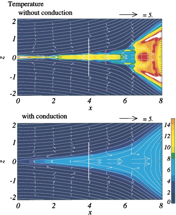
Figure 1. Temperature maps shown without (top) and with (bottom) conduction, from Yokoyama & Shibata (1997). The vertical line shows the approximate location at which parameters were measured, while arrows show flow velocity vectors. (Figure from Yokoyama & Shibata 1997, used with permission.)
Download figure:
Standard image High-resolution image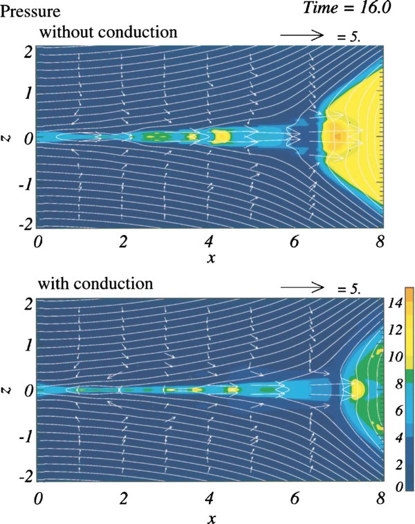
Figure 2. Pressure maps shown without (top) and with (bottom) conduction, from Yokoyama & Shibata (1997). (Figure from Yokoyama & Shibata 1997, used with permission.)
Download figure:
Standard image High-resolution image
Figure 3. Cross sections showing the variation of density (left) and temperature (right) across the thermal halo and current layer in Yokoyama & Shibata (2001). The dark shaded region represents the thermal halo region, the light shaded region represents the locations of the slow shocks which surround the current layer. (Figure from Yokoyama & Shibata 2001, used with permission.)
Download figure:
Standard image High-resolution imageIt is clear from these figures that conduction notably changes the behavior of the plasma near the current layer. In addition to increasing its temperature, conduction also affects the flows and magnetic field in this layer, accelerating the tangential flow while reducing the tangential field. Therefore, in order to understand the full effects of thermal conduction, it is necessary to model the effect of thermal conduction on the thermal halo surrounding the current layer, as well as the current layer itself.
Somov & Oreshina (2000) have previously done a rough analysis of how thermal conduction modifies the reconnection process (based on a reconnection model by B. Somov and V. S. Titov described in Section 2) but their analysis is too simple to allow direct comparison with numerical simulations like those of Yokoyama & Shibata (1997, 2001). Somov and Oreshina treat the thermal conduction in their model as a simple energy loss term, and do not consider the effects of heat flow out of the current sheet on the surrounding plasma. Consequently, their model mixes together the halo and the jet regions, so that they do not accurately predict the properties of either region. In this paper, we offer a more complete model, where we do consider the effects of heat flowing out of the current layer on the plasma that surrounds it. This allows us to make a better comparison between the results of our own modeling efforts and other numerical models, which consider both the current layer and surrounding regions.
2. THE SOMOV AND TITOV MODEL
Since all contemporary coronal mass ejection (CME) and solar-flare models depend on magnetic reconnection in order to convert energy stored in coronal fields into heat and kinetic energy, the question of exactly how the process of reconnection unfolds is an important and well studied problem. There are several analytic models of reconnection, the most famous of which are the models of Sweet (1958) and Parker (1957) and the Petschek (1964) model.
In this treatment of the steady-state two-dimensional reconnection problem, we use a technique by B. Somov and V. S. Titov (Titov 1985a, 1985b; Somov et al. 1987; Somov 1992). This approach returns the variation of averaged quantities along the length of the current layer, which consists of both the diffusion region and the slow-mode, Petschek-type shocks. The advantage of working with average quantities is that one can reduce the full set of two-dimensional MHD equations to a set of one-dimensional equations. The primary disadvantage is that information about the internal variations across the layer are lost.
Their approach to the reconnection problem makes use of a common procedure for the analysis of fluid flow through a nozzle. Perhaps the best known example, found in many fluid dynamics textbooks, is the analysis of the de Laval nozzle. This is an hourglass-shaped nozzle that is used to accelerate fluid flow to supersonic speed (Leipmann & Roshko 1957, pp. 124–130; Schreier 1982, pp. 46–57). The standard textbook treatment averages the flow over the width of the nozzle, thereby reducing the problem from two dimensions to one. This approximation is valid as long as the width of the nozzle is small compared to the scale of the variation of the thickness along the nozzle. The principal difference between this approach and the Somov–Titov approach, however, is that a nozzle has a definite profile, and thus there is a known function that describes the width of the nozzle as a function of the distance along it. In Somov and Titov's treatment of reconnection flow, the current layer's shape is not known—its thickness depends on how the other parameters act on it. Thus, an additional assumption about the character of the reconnection layer must be imposed in order to obtain a solution for the one-dimensional system. In fact, this aspect of the problem also has a counterpart in nozzle flow: once the flow from a nozzle exits into free space, it is bounded by shocks whose shape and location are not known. Nonetheless, the one-dimensional treatment can still be used in this region to provide some useful results (see pp. 127–130 of Leipmann & Roshko 1957).
In order to solve the reconnection problem, Somov begins with the complete set of steady-state two-dimensional MHD equations. These equations, given by Roberts (1967), are the continuity equation,
the momentum equation,
where
the energy equation,
where
and Ohm's Law,

Here, xi are the planar Cartesian coordinates, ρ is the density of plasma, V is a vector representing the velocity of flow, p is the gas pressure, Mij is the Maxwell stress tensor (for a plasma), B is the magnetic field, κi,j is a conduction coefficient, T is the plasma temperature, c is the speed of light, E is the electric field, j is the electric current, γ is the ratio of specific heats (taken, throughout this paper, to be 5/3), and σ(x) is the electrical conductivity.
2.1. Key Assumptions
Because Somov (1992) did not describe the procedure used to obtain the averaged equations in detail, we believe it is worthwhile to examine procedure and assumptions used to generate these equations. However, before we apply the averaging approach used by Somov (1992), it is useful to introduce some of the notation and assumptions we will use below. First, we compute averages by integrating each term of the MHD equations over the half-thickness, a(x), of a current layer centered along the x-axis, so that, for example,
where y is the direction normal to the layer and 〈Q(x)〉 is the average value of some function Q(x,y). The location y = a(x) corresponds to an external point, just outside of the layer. This point represents the division between the potential field region where there is no current density, and the nonpotential current layer itself, where current density is not necessarily zero. That is, for locations where y>a the magnetic field is potential, while for locations where y < a there is some current density. This current density may be spread uniformly throughout the layer, as in the diffusion region, or may be bifurcated into shocks, as in the Petscheck shocks region. Note that in the diffusion region, the dynamics are dominated by plasma diffusion (the η j term) while in the shocks region, dynamics are dominated by the V × B term.
Because every quantity that remains after averaging is a function of x only, we will simplify our notation by dropping the (x) from here on. Subscripted variables such as Vya will indicate boundary values at a. Subscripted variables such as Vy0 indicate values at the center of the layer at y = 0. Finally, following the standard practice for nozzle flow, we assume that quantities defined inside the current layer are uniform across the layer, allowing us to rewrite averages of products as products of averages, so
(Here, Q and R represent two arbitrary variables which have been averaged using the procedure above.)
In order to evaluate boundary terms in averaged equations, we need to know the properties of the plasma outside of the current layer. Most of these properties are the result of the inherent symmetry of the current sheet to be considered. Working with the configuration shown in Figure 4, we suppose the following properties hold: the current layer is much thinner than the scale of the variations in x along the layer, the field and flow configuration has the fourfold symmetry and antisymmetry properties shown in Figure 4, the dominant contribution to the magnetic field outside the current layer is Bx, the density in the current layer is nearly uniform across the layer, hence ρ0 = 〈ρ〉, and terms of order 2 and higher in Alfvén Mach number, MA, can be dropped.
Figure 4. Schematic of the field and flow configuration used in the Somov–Titov approach. The shaded region, with thickness a(x), represents the current layer, while the shading indicates the approximate location of heated plasma. Field is carried into the current layer from the top and bottom, reconnects, and is ejected in two oppositely directed jets in the x-direction.
Download figure:
Standard image High-resolution imageThe assumptions about the symmetry have particular consequences for several quantities along the axes. Because the magnetic field in the x-direction reverses as one crosses the x-axis, Bx0 = 0. Similarly, because the incoming flow above the x-axis is in the negative direction while incoming flow below the x-axis is in the positive direction, the flow in the y-direction must reverse sign at the x-axis, thus Vy0 = 0. We will make use of both of these facts when we derive the averaged MHD equations below.
This treatment involves the use of several parameters: the inflow Alfvén Mach number, MA, the plasma beta, β, and the Lundquist number (or magnetic Reynold's number), Lu, and the normalized thermal conductivity coefficient, λ. We normalize each equation so that solutions depend only on these four input parameters. Table 1 shows how each physical quantity is normalized.
Table 1. Normalization of Physical Quantities
| Quantity | Symbols | Normalization |
|---|---|---|
| Magnetic field | B | B0 |
| Velocity | V |  |
| Density | ρ | ρa |
| Pressure | p | B20/4π |
| Length | x | L |
Note. B0 and ρ0 are the magnitude of B and the value of the density at x = 0, y = a. L is the length of the current layer.
Download table as: ASCIITypeset image
2.2. Derivation of the Somov–Titov Equations
We begin our derivation of the Somov–Titov equations by taking the average of the continuity equation (Equation (1)). Integrating it across y leads to
Here, we have integrated the left-hand side of the equation directly and have applied Leibniz's Rule in order to move the derivative outside the integral on the right-hand side. Because Vy0 = 0 by symmetry, we can eliminate the second term on the left. Then, deconvolving the integral in the first term on the right-hand side and noting that ρa is normalized to 1 everywhere (see Table 1), we obtain
Before taking the average of the momentum equation (Equation (2)), we divide it into x- and y-components. In normalized units, we now have,
and
Averaging over the x-component of the momentum equation (Equation 7) gives us
where we have used integration by parts on the left-hand side of the equation, and Leibniz's Rule on the bracketed term on the right-hand side. On the left-hand side, we can immediately simplify the bracketed term, because we know that Vy0 = 0 by symmetry. We can apply Equation (1) again and rewrite the left-hand side of the equation
where we have used Leibniz's Rule to complete the integral.
To evaluate the right-hand side, we will make use of the y-component of the momentum equation (Equation 8), which, after averaging, can be straightforwardly written as
Since the kinetic energy density of the inflowing plasma is of second order, the total pressure (gas plus magnetic) must be balanced in the y-direction everywhere. Therefore, p0 = 〈p〉. By averaging Gauss's Law for magnetic fields, and assuming that By is essentially uniform in the current sheet (i.e., By0 = 〈By〉), we find a relationship between Bya and the other quantities in the momentum equation,
Carrying out the integration on the right-hand side and applying Leibniz's Rule one more time, we obtain
Since 〈By〉 and Bya are proportional to MA, the squared terms 〈By〉2 and B2ya are of second order and are therefore eliminated. Applying Equations (9) and (10), we obtain
Somov et al. (1987) and Somov (1992) originally treated the case of reconnection using a relatively simple energy equation whose only source term is Ohmic heating. More recently, Oreshina & Somov (1998) and Somov & Oreshina (2000) have considered the effect of radiative losses and thermal conduction. Before reconsidering thermal conduction in Section 3, we first consider the simpler Somov–Titov equations.
Integrating both sides of Equation (3) above yields
Here, E is the electric field, which is constant everywhere and normalized to VA0B0/c. The integration on the right-hand side can be carried out directly. Noting that Vy0 and Bx0 must be zero by symmetry, and that V3ya is a third-order term that can be neglected, the right side becomes
We use Leibniz's Rule on the left-hand side, and rewrite the averaged equation
Terms containing 〈Vy〉2 and V2ya have been dropped because they are of second order in MA. At the boundary of the current layer, in our normalized units, the electric field can be written as E = VyaBxa = MA (since Bxa = 1 where x = 0 and Vya = MA at this point) so the energy equation becomes
Finally, we can rearrange and expand Ohm's Law and average it,
Note that the term containing that By is of higher order than any of the other terms, and is therefore dropped. Also note that, because the electric field is uniform in the two-dimensional steady-state flow, integrating the first term on the right-hand side simply yields aE. We can then integrate the entire equation directly, to find
Although neither 〈Bx〉 nor 〈Vy〉 in the second term on the right is necessarily zero in general, this term is negligible for the type of reconnection flows considered by Somov and Titov. In the diffusion region, 〈Vy〉 is negligible by definition since a is defined here as the location in y where the diffusive electric field dominates. Outside the diffusion region, 〈Bx〉 is negligible. Thus, we neglect this term entirely. Finally, using that E = MA again and that Lu = c2/σ we can find the final form of Ohm's Law,
2.3. Additional Assumptions
The assumptions made so far are fairly general ones that concern the geometry of the current layer and the ordering of quantities involved. In deriving their solutions, however, Somov and Titov have made several additional assumptions that restrict the set of possible solutions to those that resemble the Sweet–Parker and Petschek-like configurations. Other types of reconnection solutions, such as stagnation point flow (Sonnerup & Priest 1975) and flux pile up (Litvinenko & Craig 1999; Priest & Forbes 2000, pp. 152–153), are eliminated by these additional assumptions. The additional assumptions that Somov and Titov make are there is no significant tangential flow outside the current layer so that Vxa = 0; the background magnetic field corresponds to that considered by Syrovatskii (1971), namely,  ; the tangential magnetic field inside the current layer is negligible, so that 〈Bx〉 = 0 to first order.
The second assumption, that the fields involved are Syrovatskii-like, is one that has been recently used by several authors (Uzdensky & Kulsrud 2000; Malyshkin et al. 2005). It represents an improvement over the assumption made by Petschek that the external field is uniform because it incorporates the length of the current layer in a natural way. The third assumption, that the tangential field inside the current layer is negligible, is based on the fact that the magnetic field between Petschek's slow-mode shocks is perpendicular to the outflow direction. This assumption allows them to close the system of equations. However, this assumption is unlikely to be valid within the diffusion region, where the expected value of 〈Bx〉 ≈ 1/2 Bxa.
Using the assumptions detailed above, Somov and Titov arrive at their averaged MHD equations: the continuity equation,
the momentum equation,
the energy equation,
and Ohm's Law,
Note that in order to solve these equations, we also make use of the pressure balance equation, which comes from Equation (9). In normalized units, this equation is
We solve this system with the computer application Mathematica 6.0.1 using the default method in the "NDSolve" routine.3 "NDSolve" finds numerical solutions to analytic systems of differential equations. As initial conditions for the solutions obtained by "NDSolve," we use explicit solutions to the equations, which can be obtained at the point x = 0.
2.4. Solutions in the Absence of Thermal Conduction
The Somov–Titov equations produce a family of solutions that depend on the choice of input parameters, MA, β, and Lu. The length of diffusion region in these solutions is approximately given by the length α, defined as
where a0 is simply a(0). Since a0 = 1/LuMA, we also have
At x = α, the diffusive electric field, Bxa/(LUMA), is roughly equal to the convective electric field, 〈Vx〉〈By〉.
The parameter α can be as small as α ≈ a0 and as large as α = αcrit, where αcrit is of order 1. Solutions with α>αcrit have an o-line instead of an x-line at x = 0. Figure 5 shows examples of each of these solutions. The four variables plotted are 〈Vx〉, 〈By〉, 〈ρ〉, and a. In the case of the small α solutions (solid curve), 〈Vx〉 and 〈By〉 characteristically rise to nearly their maximum outflow values quickly inside the diffusion region, then remain relatively constant through the shock region, much like the Petschek solution. The thickness of the current layer, a, also increases in a manner expected for the slow shocks present in the Petschek model. The solutions' tendency away from Petschek-like behavior as they approach the end of the current layer is due to the decrease in Bxa of the Syrovatskii background field. This effect is absent from Petschek's solution because of its use of a uniform background field (i.e., Bxa = −1).
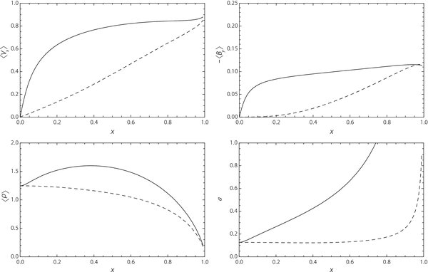
Figure 5. Two possible solutions to the Somov–Titov system for an inflow Alfvén Mach number MA = 0.1. The solid line is a Petschek-like solution, with Lu = 1000, and thus α = 0.1, while the dashed line is a Sweet–Parker-like solution with Lu ≈ 80 and α ≈ 1.25.
Download figure:
Standard image High-resolution imageIn the case of a Sweet–Parker-like solution where α ≈ 1 (dashed line), 〈Vx〉 and 〈By〉 do not achieve their maximum outflow values until they reach the end of the current layer, which, in this case, is also the end of the diffusion region. When α is slightly greater than 1, 〈By〉 increases as x3. (In Figure 5, we have chosen Lu so that 〈By〉 behaves in this way.) This choice of α produces the most sheet-like solution, and we refer to the value of α that produces it as the critical α. This is the value αcrit discussed above.
3. THE EFFECTS OF THERMAL CONDUCTION
Figure 6 shows a schematic of the configuration of the current sheet and slow shocks when a thermal halo is present. Because we wish to compare directly with the results of Yokoyama and Shibata, we will use the classical formula for the heat flux term derived by Spitzer (1962). That is,

where κ is the thermal conduction tensor,  is the energy loss function, and T is the temperature.
Figure 6. Schematic of the configuration of the current layer and thermal halo in this reformulation of the Somov–Titov system including thermal conduction. The addition of conduction creates flow and variation in the magnetic field along the boundary at a(x) that are calculated using a modified version of the shock properties determined by Xu & Forbes (1992).
Download figure:
Standard image High-resolution imageThe classical form of the heat conduction term assumes a high degree of particle collisions, and the rate of particle collisions in a typical flare current sheet are expected to be too low for the classical formula to be applicable (Somov 1992). The maximum heat flux that a collisionless plasma can carry is strongly limited by the number of electrons within the plasma. If collisions are infrequent, then the heat flux cannot exceed the free streaming limit of the electrons (Battaglia et al. 2009). Furthermore, it may also be limited by ion-acoustic turbulence to even lower values (Gray & Kilkenny 1980). In Section 5, we will discuss the effect of using a more realistic flux limited conduction formula in place of the classical one.
We assume that conduction occurs only along magnetic field lines and that conduction along the field is proportional to T5/2. Because we have already assumed that pressure and density are uniform in the y-direction inside the current layer, the temperature is also uniform in this direction. Therefore, all of the conduction in our model takes place in the halo region that connects to the chromosphere. In the region between the slow shocks, the magnetic field has only a By component, perpendicular to the current layer, so there is no conduction along the jet in this region.
To obtain a better estimate of the actual temperature gradients in the external region requires a full two-dimensional model of the entire flare loop-chromosphere system. Such a model is beyond the scope of our analysis here, which is focused on the current layer region. The estimated energy lost to thermal conduction can, therefore, be written as
Here, θ is the angle between the magnetic field and current layer, which appears as a consequence of the tensor product in the general form of  . λ is a constant, based on the Spitzer formula (Priest 1982), so
For simplicity, the ∇ operator can be approximated by (T7/2 − T7/2sink)/Lc, where Tsink is the effective temperature of the chromosphere and Lc is the distance to the chromosphere. We can also rewrite the tangent term as the ratio 〈By〉/Bxa. We can then rewrite the conduction term in our normalized units,
where λ* is the normalized thermal conduction coefficient, into which we have absorbed all the constants in the equation. λ* is given by
The constants T0, ρ0, and VA0 are the ambient temperature, density, and Alfvén speed, measured upstream of the current layer at x = 0.
The dimensionless parameter λ* represents the ratio of the energy loss due to thermal conduction to the energy input by Poynting flux carried at the Alfvén speed into the current layer. Here, λ* must be in the range of approximately 0 ⩽ λ* ⩽ 1. (In fact, it is possible to choose parameters such that λ*>1, but because the sheet cannot cool beyond the background temperature, any such choice returns the same solution as when λ* = 1.) Since 〈By〉 goes to zero as one approaches the x-line, Equation (22) would imply that there is little thermal conduction in the diffusion region. However, the above expression is not valid in this region, because the field there is parallel to the flow (see Yokoyama & Shibata 1997).
3.1. Equations for Reconnection Jet within a Thermal Halo
The main consequence of adding thermal conduction to our model is that heat can now flow out of the central current layer and into the halo region. In order to model the transition from the jet to the halo, we need to model the interface between the two. In general, this is a very complex problem, but the problem is considerably simplified when slow-mode shocks are present. The structure of slow-mode shocks in the presence of thermal conduction and radiation has been previously considered by Xu & Forbes (1992). However, they did not include any effect of energy lost by conduction to the chromosphere.
The addition of thermal conduction modifies the boundary values upstream of the shock, so that Vxa and Bya in the Somov and Titov equations are no longer zero. Thermal conduction also raises the temperature of plasma immediately upstream of the slow shock so the shocks become isothermal. Xu and Forbes provide general relationships for the shock transition in the presence of an energy loss of any type. In the switch-off limit, these relations are

where the dimensionless parameter I0 is the ratio of the energy loss rate to the incoming Poynting flux. In Xu & Forbes (1992), I0 is just the energy loss due to radiation. One key difference between our treatment of the slow-mode shock with heat conduction and the Xu and Forbes treatment is that the reconnection current layer is two-dimensional, while theirs was only one-dimensional. In the Xu and Forbes model, all heat that is conducted into the upstream region is necessarily convected back downstream (since, with only one dimension, there is no way to remove heat from the system entirely). In our model, heat can escape the system entirely if it flows to the heat sink before convection can carry it back into the current layer. Thus, there is always a net energy loss in our model and the ratio I0 becomes
Here, we use 〈T〉 = (2〈p〉)/(β〈ρ〉) and the isothermal condition that the temperature must be the same both inside and outside of the current layer. The background field outside the halo is unchanged from before, but we now have three regions: the central high-speed reconnection jet, the thermal halo, and the background. To differentiate among these three regions, we use the subscript a—e.g., Bxa—to signify quantities in the halo, at the location a, immediately upstream of the jet, and the subscript u—Bxu—to signify quantities in the far upstream region. Thus, we now refer to the background field as Bxu.
Since the relative heat loss, I0 depends on the properties of the jet, we need to iterate the combined system of slow-shock jump conditions and the Somov–Titov current layer. We first obtain an internal solution without including loss terms, then use this internal solution to find the appropriate shock jump conditions using Equations (23)–(28). Next, we use these new jump conditions to obtain the boundary conditions for the Somov–Titov system. This procedure is repeated until the solution converges.
Bearing in mind the iterative nature of the solution, and using the relationships above, we can rewrite the averaged MHD equations, as
for the continuity equation;
for the momentum equation; and
for the energy equation. Ohm's Law is unchanged from its previous form.
We again obtain explicit analytic solutions to the equations at x = 0, which we use as the initial conditions for obtaining solutions numerically for the rest of the layer. However, as we mentioned before, the solution within the diffusion region (the region where x < α) is not valid. Because the Xu & Forbes (1992) equations hold only for slow shocks, and the slow shocks are not present in the diffusion region, the solutions including the effects of these shocks are only meaningful in the region outside the diffusion region (x>α). We also note that the Xu & Forbes jump conditions hold only in the case that the thickness of the subshock transition across the interface is much less than the halo thickness—that is, the subshock thickness must be much less than the total shock thickness.
3.2. Solutions
Because, in our formulation, thermal conduction removes energy from the system, the most immediate consequences of adding thermal conduction are to cool and slow the outflow jet in the current layer. Figure 7 shows the effect of increasing thermal conduction given an otherwise identical set of input parameters. The top plot shows the speed of the outflow jet, 〈Vx〉, the middle plot shows the temperature, 〈T〉, of the current layer, while the bottom plot shows the density of the current layer, 〈ρ〉. In the case with no thermal conduction (red curves), the outflow jet nearly reaches the Alfvén speed at the end of the current layer. Additionally, because there is no cooling, the temperature of the current layer is relatively uniform and very high. In the case with modest thermal conduction (green curves), the outflow jet reaches only about 80% of the Alfvén speed, and, because some heat is carried out of the current layer by conduction, the temperature cools by nearly a factor of 10. In the case with maximum conduction (that is, the largest value of λ for which we can still obtain solutions), indicated by blue curves, the outflow jet reaches only about 50% of the Alfvén speed, and the temperature is almost uniformly equal to the background temperature. The dashed portion of the curves refers to the diffusion region solution, where the Xu & Forbes (1992) equations do not hold.

Figure 7. Effect of different thermal conductivity levels on the variation of outflow speed, temperature, and density with distance x along the current layer. The red curve corresponds to no conduction, the green to a modest amount of conduction, and the blue to very high conduction. The curves are dashed inside of the diffusion region, where the solutions including thermal conduction are not valid.
Download figure:
Standard image High-resolution image4. COMPARISON WITH NUMERICAL SIMULATIONS
The numerical simulations by Yokoyama and Shibata were motivated by earlier predictions by Forbes et al. (1989) that the strong thermal conduction that exists in the corona would modify the standard Petschek configuration by replacing the slow MHD shocks with a combination of conduction fronts and isothermal slow-mode shocks. The basic idea was confirmed by Yokoyama & Shibata (1997). However, we have carried out a detailed comparison between their simulation and the isothermal slow-mode jump conditions and have found discrepancies on the order of a factor of 2 between the analytical and numerical results. As we will discuss, these discrepancies are due to the fact that the jump relations of Xu & Forbes (1992) must be modified to include the energy lost by conduction of heat away from the reconnection region to the chromosphere. Such a loss always occurs in a two-dimensional reconnection configuration. Here, we will show that once this loss is incorporated into the shock jump relations, a good agreement between the numerical and analytical results is obtained (see Tables 3 and 5).
In order to evaluate our model, we compared it to the two numerical models by Yokoyama & Shibata (1997, 2001) described in Section 1. These two-dimensional models make use of a numerical code that includes nonlinear, anisotropic heat conduction. Unlike our steady-state model, these simulations are time dependent, so our benchmarking comparison corresponds only to a snapshot of their model at some point in its evolution. These simulations do evolve into relatively steady configurations, but low-level fluctuations are always present.
Yokoyama & Shibata (1997, 2001) use a classical Spitzer-type conduction coefficient that is proportional to T5/2∇T, so we have used the same form so as to facilitate a good comparison. In real flares, the thermal conduction is likely to be anomalous because of the very high temperature of the flare plasma. As we have previously mentioned, an important difference between the Somov & Oreshina (2000) model and the Yokoyama & Shibata simulation is the presence of a tangential field (Bx) inside the current layer. Because Somov and Oreshina assume that 〈Bx〉 is zero everywhere, the conductive loss goes to zero at their x-line. However, in the Yokoyama & Shibata model, heat flows not only out of the current layer and into the surrounding plasma, but also flows along field that exists in the diffusion region. Consequently, Somov & Oreshina (2000) predict very high temperatures in the diffusion region that simply do not occur in numerical simulations. If anything, the temperature in the diffusion region in the simulations is cooler than the rest of the layer. Thus, it is clear that the Somov–Titov formalism can only be used to model the effects of thermal conduction outside the diffusion region, where normal field dominates any tangential field. In this region, conduction in both models is predominantly out of the current layer (rather than along it).
In order to make the comparison to our results, we have estimated average values of key parameters in the Yokoyama and Shibata model both inside the current layer and at the boundary in the thermal halo region. This estimation is done by visually inspecting plotted cross sections from the two Yokoyama & Shibata (1997, 2001) papers (see Figures 1–3). Most of the small-scale variations seen in these plots are due to temperature fluctuations. Nonetheless, in most cases it is possible to estimate an average value, treating the fluctuations as a measure of the error in the estimate. These cross-sectional measurements are made well outside the diffusion region in both cases (in the location of the white line in Figure 1), where our analytic model should be valid.
We can see in Figures 1 and 2 that conduction has a significant effect on the results of the simulation, most obviously, broadening the heated region and increasing the uniformity (in temperature and other parameters) of the current layer. The expansion of the heated region occurs because heat flows out from the hot current layer and into the surrounding plasma, creating—as we have discussed above—a thermal halo. The increase in uniformity occurs because heat flows along lines of magnetic field faster than the plasma would otherwise naturally diffuse. Thus, without conduction, small regions of plasma can be heated to high temperatures, and there is no mechanism to cool them or spread the thermal energy into the surrounding plasma. With conduction, even if heating only occurs in a particular region, heat can quickly flow throughout the entire current layer and thermal halo, leading to an even distribution of temperature.
We compared our results to the Yokoyama and Shibata results by measuring plasma parameters inside the current layer and thermal halo and comparing the relative values of each. Tables 2 and 3 show the input parameters used to match those in Yokoyama & Shibata (1997) and a comparison of ratios inside and outside the current sheet for the two models. Tables 4 and 5 show the same values, respectively, for comparison with Yokoyama & Shibata (2001). Error in the measurements of the Yokoyama & Shibata results arises from both the time-varying nature of their solution (which leads to many small fluctuations throughout the current layer that make it impossible to assign an exact average value at any location) and the fact that values are read off of a graph with limited resolution. Fluctuations throughout the solution, however, account for the bulk of the error, which was estimated by eye.
Table 2. Input Parameters of the Yokoyama & Shibata (1997) Simulations
| Physical Parameter | Symbol | Value |
|---|---|---|
| Cooling length scale | Lc | 6 × 10⁸m |
| Particle number density | n0 | 1 × 10¹⁵m−3 |
| Background magnetic field | B0 | 21.7G |
| Background temperature | T0 | 4 × 10⁶K |
| Plasma β | β | 0.03 |
| Conduction coefficient |  |
3.4 × 10⁻⁴ |
| Alfvén Mach number | MA | 0.1 |
| Lundquist number | Lu | 3.6 × 10³ |
Download table as: ASCIITypeset image
Table 3. Comparison of Ratios Calculated from Yokoyama & Shibata (1997) and the Corresponding Two-Dimensional Analytical Model
| Physical Parameter | Symbol | Y&S '97 Model | Theory |
|---|---|---|---|
| Density ratio | ρa/〈ρ〉 | 0.20 ± 0.04 | 0.34 |
| Pressure ratio | pa/〈p〉 | 0.20 ± 0.02 | 0.30 |
| Velocity ratio | Vxa/〈Vx〉 | 0 ± 0.2 | 0.15 |
| Magnetic field (x-direction) ratio | Bxa/B0 | 0.88 ± 0.04 | 0.85 |
| Magnetic field (y-direction) ratio | Bya/〈By〉 | 1.10 ± 0.07 | 1.4 |
Download table as: ASCIITypeset image
Table 4. Input Parameters of the Yokoyama & Shibata (2001) Simulations
| Physical Parameter | Symbol | Value |
|---|---|---|
| Cooling length scale | Lc | 6 × 10⁷m |
| Particle number density | n0 | 1 × 10¹⁵m−3 |
| Background magnetic field | B0 | 5.9G |
| Background temperature | T0 | 2 × 10⁶K |
| Plasma β | β | 0.20 |
| Conduction coefficient |  |
0.015 |
| Alfvén Mach number | MA | 0.1 |
| Lundquist number | Lu | 1 × 10⁴ |
Download table as: ASCIITypeset image
Table 5. Comparison of Ratios Calculated from Yokoyama & Shibata (2001) and the Corresponding Two-Dimensional Analytical Model
| Physical Parameter | Symbol | Y&S '01 Model | Theory |
|---|---|---|---|
| Density ratio | ρa/〈ρ〉 | 0.48 ± 0.03 | 0.52 |
| Pressure ratio | pa/〈p〉 | 0.47 ± 0.02 | 0.45 |
| Velocity ratio | Vxa/〈Vx〉 | 0.11 ± 0.01 | 0.18 |
| Magnetic field (x-direction) ratio | Bxa/B0 | ⋅⋅⋅ | 0.82 |
| Magnetic field (y-direction) ratio | Bya/〈By〉 | ⋅⋅⋅ | 1.4 |
Download table as: ASCIITypeset image
We can clearly see from the tables, there is systematic agreement between our analytical model and the MHD simulations. In general, the ratios measured in the Yokoyama & Shibata (1997, 2001) model were within about 20%–30% of the same ratios measured in our model, although there are a few cases where there are larger differences. The most notable of these is the velocity ratio in the 1997 paper, which, because of rapid fluctuations in the thermal halo region, was difficult to measure. In this case, however, measurements of the same ratio in the 2001 paper confirm that our results appear to agree. Additionally, Yokoyama & Shibata do not include cross-sectional plots of magnetic field in their 2001 paper, thus these ratios are omitted from our comparison.
It is important to note that, while both models treat the shock and thermal dynamics similarly, there are a few major differences. Most obviously, Yokoyama & Shibata include two-dimensional effects in their model that ours cannot accommodate. It seems likely that two-dimensional effects account for the bulk of the difference between the two models. Other factors that may contribute to the differences are the numerical noise and the presence of non-steady-state features in the Yokoyama and Shibata model.
5. FAST SHOCK FORMATION IN THE PRESENCE OF CONDUCTION
During flares, hard X-ray emission is often observed co-located with the tops of the postflare loop arcade (Sui et al. 2002). These X-ray emissions may be caused by particle acceleration due to a fast-mode shock termination that forms in the reconnection outflow jet above the postflare loop systems (Tsuneta & Naito 1998; Mann et al. 2001; Mann & Klassen 2005). The effectiveness of such a shock in accelerating particles is closely related to the fast-mode Mach number, MFM, of the shock. Theory and simulations (see Forbes 1986) predict that for Petschek-type reconnection MFM should be less than  for γ = 5/3. Such a low value of MFM is marginal from the point of view of shock acceleration theory (Mann & Klassen 2005). As we will see, thermal conduction acts to increase the Mach number and thereby makes it more effective as a source of energetic particles.
In our normalized units, we can calculate the fast-mode Mach number of the outflow jet using the formula
where the numerator is the outflow speed in the jet and the denominator is the fast-mode wave speed in the direction of the flow. Because 〈By〉 is of order MA in the jet, the fast-mode Mach number is nearly the same as the sonic Mach number. Since the highest value of MFM occurs near the tip of the current layer, we measure the fast-mode Mach number at the point 1 − MA. Beyond this location, our assumptions break down as Bxu approaches zero at the tip of the Syrovatskii current layer (see Section 2). Measuring at this point generally allows us to calculate the Mach number for the fastest flow, and therefore returns the maximum Mach number for a given set of parameters. Figure 8 shows an example of the behavior of fast-mode Mach number as a function of the distance along the current layer. The Mach number is generally low in the diffusion region, then rises rapidly in the shocks region as the temperature cools and the flow reaches its maximum speed.
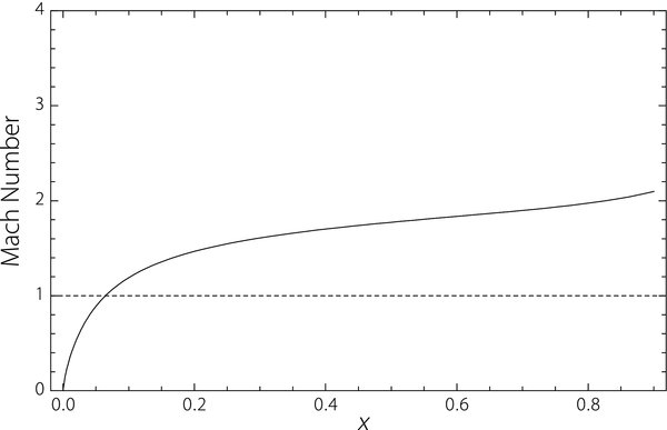
Figure 8. Example of the fast-mode Mach number shown as a function of distance along the current layer, x, plotted for the case corresponding to the Yokoyama & Shibata (1997) input parameters that appear in Table 2. The dashed line corresponds to a Mach number of 1, and shows where the flow becomes super-magnetosonic.
Download figure:
Standard image High-resolution imageBased on thermal conduction's effect on outflow jet speed, one might expect that increasing thermal conduction would simply reduce the outflow jet's fast-mode Mach number, and thus the strength of the shock in the outflow jet. However, the Mach number also depends on the fast-mode wave speed. Increased thermal conduction acts to cool the jet, which in turn reduces the local fast-mode wave speed. The net effect is to increase the fast-mode Mach number. To show this result, we plot the fast-mode Mach number as a function of the normalized conduction coefficient λ* and plasma β (Figures 9 and 10, respectively). For a given plasma β (denoted by color in both figures), as conduction coefficient rises, the Mach number increases to a certain value, then decreases slightly, as is evident in Figure 9. As the normalized conduction coefficient becomes much larger than unity, the Mach number approaches an asymptotic limit.
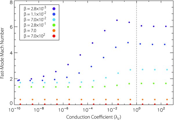
Figure 9. Effect of conduction coefficient on fast-mode Mach number. The colored dots correspond to different plasma β cases, which are identified in the inset in the upper left. The dashed vertical line shows where the effect of increasing conduction ceases to have an effect. (Once the plasma is cooled to the background temperature, it cannot cool any more and conduction switches off.) The peak in Mach number occurs when conduction is slightly less than maximum.
Download figure:
Standard image High-resolution image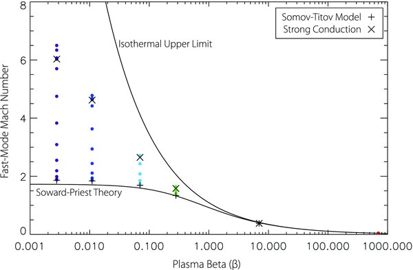
Figure 10. Effect of plasma β on fast-mode Mach number for the same individual cases as shown in Figure 9. Cases with low Mach number correspond to low conduction, while cases with large Mach numbers correspond to high conduction. The "+" signs indicate Mach numbers calculated for the Somov–Titov case with no conduction, and the "×" signs indicate a Somov–Titov-like case where the energy equation is replaced by the assumption that the plasma in the sheet has cooled to the background temperature. The two curves refer to the theoretical limits for Mach numbers: the lower one is the Soward & Priest (1982) calculation of Mach number without conduction, while the upper curve is the Mach number for a flow at the Alfvén speed in an isothermal plasma.
Download figure:
Standard image High-resolution image
The normalized conduction coefficient is equal to the ratio of the energy outflow due to thermal conduction to the energy inflow of the Poynting flux, as defined in Section 3. A conduction coefficient greater than one corresponds to cases where nearly all the incoming magnetic energy in the system is being removed by heat flow. As we noted before, a conduction coefficient greater than one does not remove any more energy from the system, so increasing the conduction coefficient beyond one has no effect on the fast-mode Mach number.
As the conduction coefficient increases, the temperature of the current layer decreases (see Section 3.2), and, correspondingly, so does the sound speed. If the sound speed decreases while the outflow speed stays relatively constant, the fast-mode Mach number increases. However, as the conduction coefficient approaches one, the temperature of the current layer approaches equilibrium with the outside, and thus the sound speed reaches a minimum. Meanwhile, as energy is lost to thermal conduction, the jet also slows. If the sound speed remains relatively constant while the outflow jet slows, the fast-mode Mach number is reduced. Thus we see—as in Figure 9—that the maximum Mach number for a given plasma β occurs when the conduction coefficient is slightly less than one.
Figure 10 shows how varying the plasma β affects the fast-mode Mach number of the outflow jet. For each β, there is a family of possible solutions, depending on the choice of conduction coefficient. We know from Figure 9 that higher Mach numbers occur when the conduction coefficient becomes large, while low Mach numbers occur when the plasma β is low. Figure 10 also shows the Mach number for several special cases. The lower curve refers to the Mach number that results from the use of the Soward & Priest (1982) reconnection theory. This theory is a compressible Petschek-type reconnection model with no thermal conduction and it predicts that  for γ = 5/3. The upper curve gives the isothermal upper limit on Mach number, assuming the outflow occurs at exactly the Alfvén speed of the inflowing plasma (i.e.,
  ). The "+" signs refer to Mach numbers calculated for the Somov–Titov theory with no thermal conduction for a given plasma β, while the "×" signs refer to Mach numbers for outflow for a modified Somov–Titov theory where the energy equation is modified to force the current layer and surrounding plasma to be entirely isothermal. We note that the results for the Somov–Titov model correspond closely to our results for zero conduction, while the strong-conduction Somov–Titov case corresponds closely to our own isothermal model. None of the low-β solutions approach the isothermal limit: the energy lost by conduction prevents the flow from reaching the Alfvén speed.
The very good agreement between our results for λc = 0 and those of Soward & Priest (1982) provides confirmation that the Somov–Titov formalism works reasonably well for Petschek-type reconnection. The Soward and Priest theory uses a completely different mathematical approach than that of Somov and Titov. It uses a rigorous two-dimensional, self-similar analysis of the compressible MHD equations. It only assumes, as we have here, and as Petschek implicitly assumed, that the length of the diffusion region is a free parameter.
Somov & Oreshina (2000) point out that for a high-temperature current sheet, heat flow may be better described by anomalous heat flux than classical heat flow, so for comparison, we also studied solutions using an alternate formulation of the energy equation where we replace the classical heat flux of term described in Section 3.1 with an anomalous heat flux term. In order to compare to the Somov & Oreshina result, we used the same formula for locally limited heat flux as they did, which is given in complete form in Somov (1992),
Here, ne is the electron density, kB, the Boltzmann constant, mi is the ion mass, and θ is the ratio of electron to ion temperatures, θ = Te/Ti. f(θ) is given by
where me is the electron mass. This formula represents the thermal flux in the presence of ion-acoustic waves. Although the significance of ion-acoustic waves in the corona has yet to be established, it is considered by some researchers (e.g., Battaglia et al. 2009) to be an important mechanism for limiting the heat flux carried by thermal conduction.
How the use of anomalous heat flow influences the rate of conduction depends strongly on the value of the coefficient f(θ), which, in turn, depends on the value of θ. If Te ≫ Ti, as Somov (1992) argues, then f(θ) ≈ 1 and the conduction is flux limited. In this case, the model behaves similarly to the Somov–Titov model shown in Figure 10, producing solutions with Mach numbers enhanced only by about 10%–20% over the no thermal conduction case. However, if Te ≈ Ti, as suggested by observations of plasma temperature in a flare by Duijveman (1983), the flux limiting of the conduction is relatively weak, and the fast-mode Mach numbers can reach values more than 60% greater than those of the no-conduction case.
We also considered the effects of heat flow at the Parker limit (see Parker 1964). Parker argued that the classical thermal flux must saturate when the heat flux equals the product of the thermal energy of the electrons and their mean thermal velocity, and thus the maximum heat flux is limited to this value. This limit corresponds to heat flux about an order of magnitude greater than the anomalous heat flux used in Somov & Oreshina's (2000) treatment, and thus cools the plasma considerably more. We found that cooling at this limit could produce Mach numbers of about 4.5 for a low-β plasma, a value about 2.5 times greater than those that occur when thermal conduction is not included (that is, the Somov–Titov and Soward–Priest models in Figure 10).
It is worth noting that the real sources of energy loss in flares are likely to be a hybrid of various mechanisms. There is some evidence to support a high-energy loss rate as a result of energetic particle acceleration. Lin et al. (2003) found evidence in RHESSI observations that significant energy loss could be attributed to energetic ions and electrons rather than thermal particles. In this (and most) cases, the form of the energy loss term is likely to be different than either of those used in this paper. However, we have found that for the production of strong shocks in the reconnection jet, the rate of energy loss is more important that the form of the loss term in the equations. Regardless of which mechanism is present, we expect strong shocks will occur any time the plasma in the jet undergoes significant cooling.
6. CONCLUSIONS
This model, including the effects of thermal conduction, can be used to interpret several observations of properties of flaring current sheets. McKenzie & Hudson (1999) and McKenzie (2000) used Yohkoh to observe postflare downflows above a reconnecting loop system in the corona and found that downflow speeds were only about half of the estimated local Alfvén speed. As a result, they concluded that the observed flows were considerably slower than those predicted by the standard reconnection models (i.e., Sweet–Parker or Petschek). However, the results shown in Figure 7 suggest that even modest conduction may reduce the speed of the outflow jet by as much as a factor of 2. Thus, we conclude that the downflows may in fact be reconnection outflow, and the relatively slow speed due to thermal conduction.
Additionally, observations of current sheet temperatures and densities by Ciaravella et al. (2002), Raymond et al. (2003), and Schwenn et al. (2006) showed that densities inside of the current layer were usually enhanced by about 2.5 times over background coronal densities, while our predictions for densities without thermal conduction remained somewhat lower than that. The addition of thermal conduction, however, allows the plasma to cool substantially, which increases its density. Even modest amounts of conduction can increase the density to five times the background as seen in Figure 7. So a small amount of thermal conduction, that might only reduce the temperature of the plasma by a few percent, may account for the higher densities observed by these authors.
An important consequence of the field-aligned conduction in this model is that the diffusion region, where the absence of tangential field restricts the flow of heat considerably, is considerably hotter than the rest of the current layer. This reveals an important feature of the reconnection simulations by Yokoyama and Shibata that has not been previously discussed: that the diffusion is relatively cool and the current sheet essentially uniform in temperature. In that case, the presence of tangential field inside the current layer allows heat to flow rapidly from the reconnection site throughout the jet. Thus, it may be possible to deduce the orientation of magnetic field inside a reconnecting current layer by observing its temperature structure.
One question left unexplored in this paper is the role that viscosity plays in determining the dynamics of the current layer. Craig et al. (2005) and Litvinenko (2005) studied the effects of viscosity in various reconnection mechanisms and found that its effects are widely variable, but suggested that viscous stress, rather than energy loss due to cooling, may be responsible for slower than expected speeds in reconnection outflows such as those observed by McKenzie and Hudson. In fact, it is possible that this effect is the result of a combination of both viscosity and conduction, since viscous dissipation could generate heat that is lost through conduction. Viscosity can, in principle, be incorporated into the Somov–Titov formalism, so this may provide an interesting topic for future research.
The research in this paper is from a dissertation by D. B. Seaton submitted to the Graduate School at the University of New Hampshire in partial fulfillment of the requirements for completion of a Ph.D. degree. This dissertation research was supported by Hinode subcontract SVT-7702 from the Smithsonian Astrophysical Observatory in support of NASA grant NNM07AA02C. Additional dissertation support was provided by the New Hampshire Space Grant Consortium and the National Science Foundation's GK-12 Program at UNH (PROBE). Support for D.B.S.'s work on this paper came from PRODEX grant No. C90345 managed by the European Space Agency in collaboration with the Belgian Federal Science Policy Office (BELSPO) in preparation of the PROBA2/SWAP mission and from the European Commission's Seventh Framework Programme (FP7/2007-2013) under the grant agreement No. 218816 (SOTERIA project, www.soteria-space.eu). T.G.F. acknowledges support from NSF grants ATM-0752257 and ATM-0518218 and NASA grants NNX-06AC19G and NNX08AG44G. D.B.S. would especially like to thank David Berghmans and the Royal Observatory of Belgium for support and encouragement during the writing of this paper.
Footnotes
- 3
The Appendix in Seaton (2008) shows the complete text of the Mathematica code used to generate these solutions, including the effects of thermal conduction, which are discussed in the next section.