


ABSTRACT
Resonant relaxation (RR) is a rapid relaxation process that operates in the nearly Keplerian potential near massive black holes (MBHs). RR dominates the dynamics of compact remnants that inspiral into an MBH and emit gravitational waves (extreme mass ratio inspiral (EMRI) events), and can either increase the EMRI rate, or strongly suppress it, depending on its still poorly determined efficiency. We use Newtonian N-body simulations to measure the RR efficiency and to explore its possible dependence on the stellar number density profile around the MBH, and the mass ratio between the MBH and a star (a single-mass stellar population is assumed). We develop an efficient and robust procedure for detecting and measuring RR in N-body simulations. We present a suite of simulations with a range of stellar density profiles and mass ratios, and measure the mean RR efficiency in the near-Keplerian limit, and explore its long-term behavior. We do not find a strong dependence on the density profile or the mass ratio. Our numerical determination of the RR efficiency in the Newtonian, single-mass population approximations, suggests that RR will likely enhance the EMRI rate by a factor of a few over the rates predicted assuming only slow stochastic two-body relaxation.
Export citation and abstract BibTeX RIS
1. INTRODUCTION
Dynamical relaxation processes near massive black holes (MBHs) in galactic centers affect the rates of strong stellar interactions with the MBH, such as tidal disruption, tidal dissipation, or gravitational wave (GW) emission (e.g., Alexander 2005). These relaxation processes may also be reflected by the dynamical properties of the different stellar populations there (Hopman & Alexander 2006), as observed in the Galactic center (Genzel et al. 2000; Paumard et al. 2006). Of particular importance, in anticipation of the planned Laser Interferometer Space Antenna (LISA) GW detector, is to understand the role of relaxation in regulating the rate of GW emission events from compact remnants undergoing quasi-periodic extreme mass ratio inspiral (EMRI) into MBHs.
Two-body relaxation, or noncoherent relaxation (NR), is inherent to any discrete large-N system, due to the cumulative effect of uncorrelated two-body encounters. These cause the orbital energy E and the angular momentum J to change in a random-walk fashion (∝ ) on the typically long NR timescale TNR. In contrast, when the gravitational potential has approximate symmetries that restrict orbital evolution (e.g., fixed ellipses in a Keplerian potential; fixed orbital planes in a spherical potential), the perturbations on a test star are no longer random, but correlated, leading to coherent (∝t) torquing of J on short timescales, while the symmetries hold. Over longer timescales, this results in resonant relaxation (RR; Rauch & Tremaine 1996; Rauch & Ingalls 1998; Section 2.2), a rapid random walk of J on the typically short RR timescale TRR ≪ TNR. RR in a near-Keplerian potential can change both the direction and magnitude of J ("scalar RR"), thereby driving stars to near-radial orbits that interact strongly with the MBH. RR in a near-spherical potential can only change the direction of J ("vector RR").
RR is particularly relevant in the near-Keplerian potential close to an MBH, where compact EMRI candidates originate. Hopman & Alexander (2006) showed that RR dominates EMRI source dynamics. Depending on its still poorly determined efficiency, RR can either increase the EMRI rate over that predicted assuming NR only, or if too efficient, it can strongly suppress the EMRI rate by throwing the compact remnants into infall (plunge) orbits (Figure 6) that emit a single, nonperiodic and hard to detect GW burst. The still open questions about the implications of RR for EMRI rates and orbital properties provide a prime motivation for the systematic numerical investigation of RR efficiency presented here.
This paper is organized as follows. In Section 2, we review the theory of NR and RR relaxation. We describe our simulations, analysis methods, and results in Section 3. We discuss the results in Section 4 and summarize them in Section 5.
2. THEORY
2.1. Noncoherent Relaxation (NR)
The NR time for E relaxation, TENR, corresponds to the time it takes noncoherent two-body interactions to change the stellar orbital energy by order of itself, |ΔE| ∼ E (by stellar dynamical definition convention, E>0 for a bound orbit). Similarly, the NR time for J relaxation, TJNR, corresponds to the time it takes the stellar orbital angular momentum to change by order of the circular angular momentum |ΔJ| ∼ Jc, where near an MBH of mass M,  . The E-relaxation timescale can be estimated by considering the rate Γ of gravitational collisions at a relative velocity v between a test star and N field stars of mass m with a space density n ∼ N/R3 in a system of size R, at the minimal impact parameter where the small angle deflection assumption still holds, rmin ∼ Gm/v2. The collision rate is then Γ ∼ nvr2min ∼ G2m2n/v3. Taking into account also collisions at larger impact parameters increases the rate by the Coulomb logarithm factor ln Λ ∼ ln(R/rmin ), so that TENR ∼ v3/(G2m2nln Λ). Near the MBH v2 ∼ GM/R, and so ln Λ ∼ ln Q, where Q ≡ M/m is the mass ratio. When the stars move under the influence of the central MBH (Q ≫ N), the relaxation time can be expressed as TENR ∼ (M/m)2P/(Nln Λ), where
  is the Keplerian period.
Rauch & Tremaine (1996, RT96) parameterized the uncertainties in the evolution of the orbital E, J, and J by a set of numeric coefficients (αΛ, ηs,v, βs,v), whose operational definition is tied to the procedure by which they are estimated (left unspecified by RT96). Here, we adopt this notation and estimate these coefficients by measuring the rms change in energy and angular momentum over the stellar population at binned time lags (Section 3.2). The NR changes in E, J, and J over the dimensionless time lag τ ≡ (t2 − t1)/P1 are thus formally defined as2


where 〈 ⋅ ⋅ ⋅ 〉 designates the average over all stars in the time-lag bin τ,  and
and  are dimensionless constants, whose exact values are system dependent. Accurate determination of their values requires detailed calculations or simulations. The corresponding NR timescales are related to these coefficients by TENR = (M/m)2P/(Nα2Λ), TJNR = (M/m)2P/(Nη2sΛ), and TJNR = (M/m)2P/(Nη2vΛ).
2.2. Resonant Relaxation (RR)
When the gravitational potential has symmetries that restrict the orbital evolution, for example, to fixed ellipses in the potential of a point mass, or to planar annuli in a spherical potential, the perturbations on a test star are no longer random, but correlated. This leads to a coherent changes ΔJ = Tt on times P ≪ t < tω by the residual torque  exerted by the N randomly oriented, orbit-averaged mass distributions of the surrounding stars (mass wires for elliptical orbits in a Kepler potential, mass annuli for rosette-like orbits in a spherical potential). The coherence time tω is set by deviations from perfect symmetry, which lead to a gradual orbital drift and to the randomization of T. For example, the enclosed stellar mass leads to non-Keplerian retrograde precession; general relativity leads to prograde precession. Ultimately, the coherent torques themselves randomize the orbits. The effective coherence time is set by the shortest decoherence (quenching) process. The accumulated change over tω, |ΔJω| ∼ |Ttω|, then becomes the basic step-size, or mean free path in J space, for the long-term (t ≫ tω) random-walk phase (
 ) of RR of J. Since this step-size is large, RR can be much faster than NR. The RR timescale TRR is then defined by
  . Note that the relaxation of E is not affected by RR because the potential of the system is stationary on the coherence timescale, and so E changes incoherently on all timescales. The torques exerted by elliptical mass wires in a Kepler potential can change both the direction and magnitude of J. In contrast, the torques exerted by planar annuli can only change the direction of J. The long-term random-walk
  growth continues until |ΔJ|/Jc ∼ O(1), at which point |ΔJ|/Jc and |ΔJ|/Jc can no longer grow, but J does continue to change its value randomly.
Here, we consider only Newtonian dynamics. The coherence timescale for scalar RR is determined by the time it takes for the orbital apsis to precess by angle ∼π due to the potential of the enclosed stellar mass ("mass precession"),

where AM is an O(1) factor reflecting the approximations in this estimate. The coherence timescale for vector RR is determined by the time it takes for the coherent torques to change by |ΔJ| ∼ Jc (self-quenching3),

where Aϕ is an O(1) factor,4 μ = Nm/(M + Nm) and where the approximate equality is for the Keplerian limit Nm ≪ M. The RR changes in J and J during the coherent phase (τ < τω) are defined in terms of the rms change as


where the dimensionless coefficients βs and βv depend on the parameters of the system and reflect the uncertainties introduced by the various approximations and simplification of this analysis. Accurate determination of their values requires detailed calculations or simulations.
The scalar RR change in J on time lags τ ≫ τM is then

and the scalar RR timescale is

The RR efficiency factor χ = (βs/βs,RT96)2 defined by Hopman & Alexander (2006) for an assumed value AM = 1 (Section 3.3), expresses how much shorter TJRR is relative to the value estimated by RT96. Scalar RR is faster than NR by a factor TJNR/TJRR ∝ (M/m)/Nln Λ. Similarly, the vector RR change in J on time lags τ ≫ τϕ in the Keplerian limit is

and the vector RR timescale is

RT96 performed a limited set of near-Keplerian simulations to check their predictions. They analyzed the results both star by star and in the average and observed the coherent growth of |ΔJ|/Jc and |ΔJ|/Jc relative to the simulation's initial values. Although the evolution of these quantities for any single star was very noisy and the proportionality factors had a very large scatter, RR was clearly observed, as predicted.
3. SIMULATIONS
3.1. N-Body Code and Models
Our N-body code uses a 5th order Runge–Kutta integrator with individual time steps and optional pairwise KS regularization (Kustaanheimo & Stiefel 1965), without gravity softening. The time steps were chosen to conserve total energy at the level of |ΔEtot|/Etot ∼ O(10−5)–O(10−8), well below the NR energy changes expected in the simulations.
To simulate RR reliably, the N-body code must maintain small-enough numerical deviations from the conserved Keplerian symmetries. These could lead to numerical quenching of RR by a drift of the orbital apsis or of the direction of the angular momentum, which change the torque felt or exerted by the orbit, and to a lesser degree by a drift in the orbital period (equivalently, the energy), which changes the shape of the orbit, and hence its moment of inertia. We estimated these numerical drifts by integrating, over many orbits, a highly eccentric two-body system (e = 0.99995, Q = 3 × 10⁶), since most of the numerical errors accumulate at periapse, where the acceleration is largest. We tracked the change in the period, ΔP = (P − P0)/P0, in the angular momentum ΔJ = |J − J0|/J0 and in the direction of the apsis  , where
  and e = v ⊗ (r ⊗ v)/(M + m) − r/|r| is the Laplace–Runge–Lenz vector. We find that after τsim = 4.5 × 10⁴, ΔP ∼ 8 × 10⁻⁵, ΔJ ∼ 3 × 10⁻⁴, and
  , which correspond to drift timescales of τΔP ∼ (π/ΔP)τsim = 2 × 10⁹, τΔJ ∼ 5 × 10⁸, and
  . These are many orders of magnitude longer than our longest simulations (e.g., Figure 5), and can therefore be safely neglected.
We carried out two sets of simulations. The first, designed to study the short-term behavior of RR (τsim < τM) and to measure NR and RR parameters α, ηs,v, and βs,v, consisted of 200 particles (including the MBH as a fixed particle, since testing showed that allowing the MBH to move did not change the results significantly, but slowed down the simulations substantially by requiring smaller time steps and KS regularization). The initial orbital semimajor axes were randomly drawn from a ρ(a)da ∝ a2−γda distribution for γ = 1, 1.5, and 1.75, for a in the range (0, 1/2), with eccentricities drawn from a thermal ρ(e)de = 2ede distribution, with random phases, orbital orientations, and isotropic velocities. This distribution approximates an r−γ number density distribution with an outer cutoff at radius r = R = 1 from the MBH (in dimensionless units where G = 1, M + Nm = 1). These stellar cusps span a wide range of possible physical scenarios (e.g., Bahcall & Wolf 1977), and in particular those of LISA targets, which are expected to be relaxed galactic nuclei (Alexander 2007). A typical simulation lasted a few × 100 system orbital times and resulted in few × 100 snapshots of the system configuration. In order to decrease the statistical errors, we ran nsim = 12–15 simulations with different initial conditions for each of the (γ, Q) models we studied.
The second set of simulations was designed to study the long-term behavior of RR (τsim ≫ τϕ), the transition from the coherent RR phase to the random-walk phase, and the asymptotic saturation limits. Due to the high computational load, this set (nsim = 7) was limited to a relatively small mass ratios, Q ⩽ 104, smaller number of particles (50 ⩽ N ⩽ 200), and flat cusps with γ = 1, where time-consuming close star-star interactions are rarer. A typical simulations lasted few × 104 system orbital times (τsim ∼ 104).
3.2. RR Detection by Correlation Analysis
Given the high computational cost of the N-body simulations, and the very large variance in the evolution of individual orbits, it is essential to extract the RR signal as efficiently and robustly as possible from the simulated data. After some experimentation, we adopted the correlation analysis for detecting and measuring RR in N-body simulation snapshots. Our procedure is as follows.
- 1.The stellar phase space coordinates are transformed to the rest frame of the MBH, which is almost identical with the center of mass in the near-Keplerian system close to the MBH.
- 2.The energy (E(n)i), angular momentum (J(n)i), circular angular momentum (J(n)c,i), and Keplerian period (P(n)i) are calculated for the nth star (n = 1...N) at discrete times ti in the simulation ("snapshots").
- 3.A normalized time lag τ(n)ji = (tj − ti)/P(n)i is assigned to each pair of times (tj>ti). For each of the N stars, we calculate the normalized energy and angular momentum differences at all lags, (|ΔE|/E)(n)ji = |E(n)j − E(n)i|/E(n)i, (|ΔJ|/Jc)(n)ji = |J(n)j − J(n)i|/J(n)c,i, and (|ΔJ|/Jc)(n)ji = |J(n)j − J(n)i|/J(n)c,i.
- 4.The differences from all stars are binned into discrete τ bins according to their associated τij. The bin rms values and their standard deviations are calculated and plotted against the bin's average time lag τ = 〈τij〉, thereby creating the correlation curve.
By using all possible time lags recorded in the simulation, this approach makes maximal use of the entire data set and averages over the strongly fluctuating individual relaxation curves (e.g., the RT96 procedure, Section 2.2). However, this method is not entirely free of bin-to-bin bias. Since the number of orbital periods completed by a star with a mean period P(n)i over the simulation time tsim is tsim/P(n) = τ(n)max , long-period stars will not contribute to a high-τ bin, 〈τ〉i if τ(n)max < 〈τ〉i. Conversely, short-period stars will not contribute to a low-τ bin, 〈τ〉i, if τ(n)min >〈τ〉i, where τ(n)min = minj(tj+1 − tj)/P(n) is set by the minimal time difference between consecutive snapshots. In extreme cases, some stars may not contribute to the relaxation curve at any 〈τ〉i. Since long- and short-period stars could well have systematically different responses to RR, this introduces bias to the relaxation curve. This bias can be reduced, at the cost of losing some information, by using only the middle range of the τ bins, or at a computational cost, by longer simulations with a higher snapshot rate.
The correlation curves δJ(τ) and δJ(τ) reflect the joint effects of NR and RR. The coefficients ηs,v and βs,v are formally defined and measured by fitting the measured correlation curves in the coherent phase to the functions
where the two terms in the square root express the contributions of NR and RR, respectively. Note that on short timescales, τ < τ0 ≡ (ηsΛ/βs)2, the RR correlation curve rises as  due to the effect of NR. It then rises as τ in the RR-dominated coherent phase at times τ0 < τ < τω, before turning over again to a
  rise in the accelerated random-walk phase at τ>τω (this last phase is not modeled by these fitting functions).
Figure 1 shows the measured correlation curves in a typical simulation for τ ≪ τω: δE(τ), δJ(τ), and δJ(τ). The NR and RR coefficients were derived from the best two-parameter fits of Equations (1), (12), and (13) to the data. To control the star to star variance, we limited our analysis to time-lag bins that sampled at least 0.75 of the stars in the simulation. The excellent fit of the data points to the predicted correlation curves seen in Figure 1 indicates that RR is present and measurable.

Figure 1. Measured (points) and fitted (lines) correlation curves for δE, δJ, and δJ in a Q = 106, γ = 1.5 simulation with N = 200 particles. The points are the results of the N-body simulation, the thick lines are the predicted theoretical curves, and the thin straight lines show the asymptotic (τ ≫ τ0) linear behavior. The best-fit coefficients and related quantities are also listed.
Download figure:
Standard image High-resolution imageTo quantify the transition between the coherent and random-walk scalar RR phases and measure the coefficient AM that sets the scalar RR coherence time (Equation (4)), and therefore the scalar RR timescale (Equation (9)), we fitted the scalar RR correlation curve up to τϕ by the composite function
where δJ(τ) (Equation (12)) is the best fit of the short timesscale NR and coherent RR phases up to τM and τb is the break timescale. The best-fit coefficient AM is then given by the best-fit break time lag, AM = (N/Q)τb.
3.3. Results
Although the correlation analysis stabilizes against star to star scatter in a single simulation, we still find a large simulation to simulation scatter in the derived values of the coefficients. We therefore constructed a large grid of near-Keplerian, short-timescale (τ0 ≪ τsim < τM) models, where coherent RR should be clearly detected.
We summarize our results in Table 1 and in Figures 2–4. The coefficients αΛ and ηs,vΛ do not directly express the intrinsic properties of NR, since they should vary as  over the Q range of our models. This small fractional difference and the relatively low statistics of our simulation suite may explain why we do not detect a clear Q dependence in these quantities. Since we do not see a dependence on Q, and the γ dependence seems weak (αΛ shows hints of an increase with γ, and η and β of a decrease with γ), we adopt as the best-fit estimates of the values of α, ηs,v, and βs,v their grand average over all the simulations (Table 1).
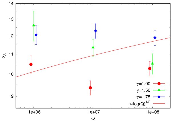
Figure 2. Measured NR energy coefficient αΛ as function of mass ratio Q and for stellar density profiles with logarithmic slopes of  . A
. A  curve is shown to guide the eye.
Download figure:
Standard image High-resolution image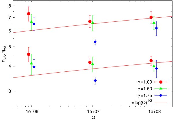
Figure 3. Same as Figure 2, for the measured NR scalar angular momentum coefficient ηsΛ (bottom points) and the vector angular momentum coefficients ηvΛ (top points).
Download figure:
Standard image High-resolution image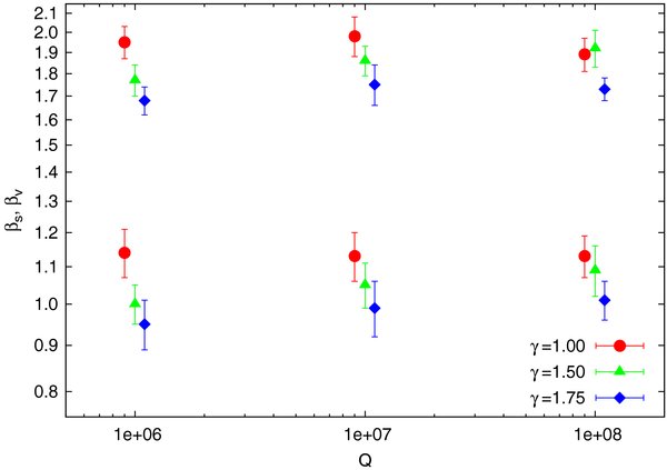
Figure 4. Same as Figure 2, for the measured RR scalar angular momentum coefficient βs (bottom points) and vector angular momentum coefficient βv (top points). Note that RR does not depend on a Coulomb factor.
Download figure:
Standard image High-resolution imageTable 1. Measured NR and RR Coefficientsa
| γ | Q | nsim |  |
 |
 |
 |
 |
|---|---|---|---|---|---|---|---|
| 1 | 106 | 12 | 10.48 ± 0.43 | 4.58 ± 0.38 | 7.31 ± 0.61 | 1.14 ± 0.07 | 1.95 ± 0.08 |
| 1 | 107 | 12 | 9.37 ± 0.32 | 4.18 ± 0.26 | 6.69 ± 0.46 | 1.13 ± 0.07 | 1.98 ± 0.10 |
| 1 | 108 | 12 | 10.27 ± 0.36 | 4.26 ± 0.22 | 7.02 ± 0.47 | 1.13 ± 0.06 | 1.89 ± 0.08 |
| 1.5 | 106 | 13 | 12.61 ± 0.90 | 4.12 ± 0.48 | 6.65 ± 0.61 | 1.00 ± 0.05 | 1.77 ± 0.07 |
| 1.5 | 107 | 12 | 11.35 ± 0.46 | 4.09 ± 0.35 | 6.58 ± 0.57 | 1.05 ± 0.06 | 1.86 ± 0.07 |
| 1.5 | 108 | 12 | 10.51 ± 0.51 | 3.99 ± 0.21 | 6.57 ± 0.49 | 1.09 ± 0.07 | 1.92 ± 0.09 |
| 1.75 | 106 | 14 | 12.06 ± 0.54 | 3.97 ± 0.35 | 6.50 ± 0.48 | 0.95 ± 0.06 | 1.68 ± 0.06 |
| 1.75 | 107 | 12 | 12.29 ± 0.43 | 3.39 ± 0.14 | 5.29 ± 0.18 | 0.99 ± 0.07 | 1.75 ± 0.09 |
| 1.75 | 108 | 15 | 11.90 ± 0.43 | 3.89 ± 0.39 | 6.20 ± 0.52 | 1.01 ± 0.05 | 1.73 ± 0.05 |
| Grand averageb | 〈α〉 | 〈ηs〉 | 〈ηv〉 | 〈βs〉 | 〈βv〉 | ||
| 114 | 2.82 ± 0.05 | 1.01 ± 0.03 | 1.64 ± 0.04 | 1.05 ± 0.02 | 1.83 ± 0.03 | ||
Notes.
aThe quoted errors are the errors on the mean (the sample rms is  times larger).
b
times larger).
b ,
,  over all simulations for Λ = Q.
Download table as: ASCIITypeset image
To explore the long-term behavior of the system, verify that the short-timescale coherent torquing phase leads to long-term relaxation (rather than oscillatory behavior, for example) and to estimate the coefficients that set the coherence timescales, we also conducted several very long simulations (τ ∼ 104 ≫ τϕ). The resulting RR correlation scalar curves display a first clear detection of a transition from the asymptotically ∝τ coherent RR phase to the ∝ RR relaxation phase (Figure 5) at the mass precession coherence time τM = AMQ/N (Equation (4)). The mean best-fit estimate (Equation (14)) over seven long-timescale simulations is AM = 0.99 ± 0.06, where the error is dominated by the simulation to simulation scatter. As discussed further below (Section 4.2), the vector RR curve does not display a coherent rise beyond τM, since by its definition it includes a scalar component, and neither does it display a distinct random-walk phase beyond τϕ, since the transition to the asymptotic saturation limit occurs soon after, at τ ≳ τϕ. This behavior makes it harder to quantify and measure Aϕ by a fit to the correlation curve, and we do not attempt it here.
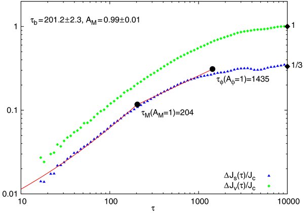
Figure 5. Long-term relaxation in a Q = 104 simulation with N = 50 particles and a γ = 1 density profile. The theoretical composite correlation curve (Equation (14)) for scalar RR (line) is fitted across the coherent (τ < τM) and random-walk phases to the simulated data (points) (see Figure 1). The theoretical estimates of τM and τϕ are shown for AM = Aϕ = 1 (Equations (4) and (5)). The derived best fit for this simulation is AM = 0.99 ± 0.01. As expected (Section 4.2), the coherent (∝τ) phase of the vector RR correlation curve extends only up to τM, and not τϕ, and it does not show a clear random-walk phase. Also shown are the theoretical asymptotic τ ≫ τϕ values of the correlation curves (diamonds) (Section 4.2).
Download figure:
Standard image High-resolution image4. DISCUSSION
4.1. Relation Between Scalar and Vector Relaxation
The relations between the correlation functions of scalar and vector relaxation, parameterized by the coefficients ηs,v and βs,v (Equations (12) and (13)), reflect the symmetries and dimensionality of the torquing process. In the limit |ΔJ|/J ≪ 1, the ratios ηv/ηs and βv/βs can be expressed as (〈|ΔJ2|〉/〈ΔJ2∥〉)1/2 = (1 + 〈ΔJ2⊥〉/〈ΔJ2∥〉)1/2, where ΔJ∥ is the change along J and ΔJ⊥ perpendicular to it, in the orbital plane.
In the case of NR relaxation, and in the limit of close (impulsive) encounters, the torquing is two-dimensional, 〈ΔJ2⊥〉 = 〈ΔJ2∥〉, and  . This can be seen by expressing dJ to leading order as dJ/Jc ≃ (dr/r) ⊗ (v/v) + (r/r) ⊗ (dv/v), where r and v are the instantaneous position and velocity of the scattered star at closest approach to the scatterer. The virial velocity in a self-gravitating system of typical size R = 1 is
  (for G = M = 1, m ≪ M) and the crossing time is tc ∼ R/V = 1. The acceleration in a two-body encounter with impact parameter b is a ∼ Gm/b2 ∼ m/b2, and the encounter time is tb ∼ b/V ∼ b. The typical change in the velocity of the interacting stars is then dv ∼ atb ∼ m/b, and in their position dr ∼ at2b ∼ m. For a typical orbit with r ∼ R = 1 and v ∼ V = 1, the ratio of relative changes due to the encounter is (dv/v)/(dr/r) ∼ 1/b. Therefore, in an impulsive, local scattering event where b ≪ R = 1, dJ/Jc ∼ (r/r) ⊗ (dv/v) is two-dimensional. In practice, however, longer range nonimpulsive encounters that last a substantial fraction of the orbit also contribute to NR. In such encounters dr/r is not negligible, dr ∼ ∫dt'∫dt a(t) and dv ∼ ∫dt a(t) are not colinear, and r(t) and v(t) change in the course of interaction. Therefore, NR is not expected to be exactly two-dimensional, and we indeed find in our simulations that 〈ηv〉/〈ηs〉 = 1.61 ± 0.06 lies between
  and
and  .
.
By contrast, in the case of RR the torquing is global, averaged over the entire orbit and exerted over many orbital periods, and the impulsive encounter argument for two-dimensional torquing does not apply. We find in our simulations that 〈ΔJ2⊥〉 ≃ 2〈ΔJ2∥〉, when averaged over a thermal eccentricity distribution, and that  . The difference from 〈ηv〉/〈ηs〉 is statistically significant, and presumably reflects the qualitatively different nature of NR and RR. However, the result 〈βv〉/〈βs〉 ≃
  is not due to isotropic torques. Rather, the decomposition of ΔJ along the normalized axes of the orbital ellipse (
 ), where
  is in the direction of the semiminor axis, reveals that 〈ΔJ2b〉 ∼ 2〈ΔJ2∥〉 ≫ 〈ΔJ2e〉. The small values of ΔJe can be understood if the residual force F acting on the mass wire is approximately spatially constant, since then the ellipse's center of mass lies along e, and the torque
  has no component along
  (e.g., Landau & Lifshitz 1976, Section 34). However, the finding 〈ΔJ2b〉 ∼ 2〈ΔJ2∥〉, and the resulting coincidental similarity to isotropic torquing when averaged over a thermal eccentricity distribution, remain to be explained.
4.2. The Long-Term Behavior of RR
The long-term behavior of the correlation curves is quite distinct from its short-term (τ < τM) behavior. Two regimes are apparent: the intermediate timescale regime (τM < τ < τϕ), when J grows by random walk, but the direction of the angular momentum  is still changing linearly with time, and the long timescale, when both the scalar and vector correlation curves reach their asymptotic saturation limits.
Intermediate timescale (τM < τ < τϕ). The vector RR correlation curve does not explicitly display a coherent (∝τ) rise beyond τM, even though the coherence time for vector RR τϕ ≫ τM. This results from the fact that as defined, δJ describes the change in both the direction and magnitude of the angular momentum. On the intermediate timescale, τM < τ < τϕ, the scalar component in δJ evolves as  , while the vector component evolves as τ. This results in a mixed behavior that is intermediate between coherent growth and random walk. This can be seen explicitly by decomposing (δJ)2 = δJ2 + 〈2(J2/J2c)[1 − cos(Δθ)]〉, where the approximations Jc = const (valid since ΔE is small for τϕ ≪ τ ≪ τNR over a wide range,
  ), and J1 = J2 = J are assumed, and where cos Δθ = J1 · J2/J2. The angle Δθ is related to δJ by
  for τ < τϕ (Equation (7)), and δJ = τ/τsRR for τ>τM (Equation (9)). It then follows that
  for τ>τM. This mixed power-law behavior further modified as τ → τϕ, δJ → 1 and the correlation curve approaches its asymptotic saturation limit.
Long timescale (τϕ < τ). When the time lag τ ≫ τϕ ≫ τM, both J and e are completely randomized and the change in the angular momentum saturates at δJ(τ ≫ τϕ) = 1/3 and δJ(τ ≫ τϕ) = 1 (Figure 5). This can be seen by considering the population rms change in the angular momentum between times τ1 and τ2, δJ = 〈(|J2 − J1|/Jc)2〉1/2 and δJ = 〈(|J2 − J1|/Jc)2〉1/2, with the approximation Jc = const. For the isotropic thermal angular momentum distribution modeled here, the parent probability density of J is ρJ = 2J/J2c for J = 0 to Jc. Assuming no correlation between J1 and J2 after long-enough time lags, and replacing the population rms by the relevant moments Ja1Jb2 over ρJ, ![$\overline{(J_{1}/J_{c})^{a}(J_{2}/J_{c})^{b}} = 4/[(2+a)(2+b)]$](https://content.cld.iop.org/journals/0004-637X/698/1/641/revision1/apj300562ieqn44.gif) , yields
, yields  and
and  , as measured.
4.3. Comparison with Previous Results
Our measured values for βs,v are in excellent agreement with the results of Gürkan & Hopman (2007), who modeled the torquing stars by the static torque field of 104 random fixed ellipses, and investigated the dependence of the RR efficiency on the eccentricity of test orbits. They report5 βs(e)/2π = 0.25e and βv/2π = 0.28(0.5 + e2), which for the thermal eccentricity distribution n(e)de = 2e modeled here, translate to 〈βs〉 = 1.05 and 〈βv〉 = 1.76 (e.g., Table 1). We note that the advantage of the full N-body approach used here, beyond verifying the approximations and assumptions that go into the fixed torques approach (orbital averaging, neglect of close encounters) is that it enables the study of the transition from and to random-walk phases, which cannot be reproduced by a fixed background. Specifically, the transition from the early NR-dominated phase to the coherent RR phase, and the subsequent transition out of the coherent RR phase to the RR random-walk phase due to quenching (especially in the case of the self-quenched vector RR, Section 2.2).
RT96 derived from their simulations smaller mean values for βs (0.53, as compared to 1.05 here) and for αΛ and ηsΛ (3.09 and 1.37 as compared to 11.25 and 4.05 here). At least part of the difference in αΛ and ηsΛ can be traced to their use of a softening length  = 10−2R ≫ Gm/v2 ∼ (m/M)R in the calculation of the gravitational force. This decreases the effective value of the Coulomb factor, since Λ ∼ R/max(, Gm/v2) = 102 and so
  , about twice as small as in our simulations. Indeed, RT96 noted that a decrease in the softening length to ε = 10−4R led to an increased value of αΛ = 5.5 ± 0.2. It is difficult to trace the specific reason for the discrepancy between our best estimate value for βs and that derived by RT96, given the many differences in both the simulations and the methods of analysis. However, we note that the statistics here are better due to the larger number of simulations, more efficient use of the data, and the more rigorous analysis.
4.4. Implications for Gravitational Wave Source Dynamics
We conclude the discussion of our results by briefly considering the implications of this revised value of βs for EMRI rates. Hopman & Alexander (2006) assumed AM = 1, parameterized the RR efficiency by a factor χ = [βs/βs,RT96]2, and derived the χ dependence of the branching ratio of the EMRI and infall (plunge) rates (Figure 6). The RT96 value χ = 1 happens to lie very close to the maximum of the RR-accelerated EMRI rate. We confirm here that AM = 0.99 ± 0.06 and find βs/βs,RT96 = 1.98 ± 0.04, which corresponds to a factor 4.9 increase in the EMRI rate compared to that estimated for NR only, but is a factor ∼1.5 smaller than implied by the RT96 value, because the higher RR efficiency leads to a higher plunge rate at the expense of the inspiral rate.
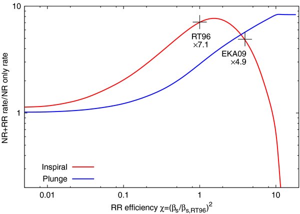
Figure 6. Change in the EMRI and plunge rates relative to that predicted assuming only NR, as function of the RR efficiency χ (adapted from Hopman & Alexander 2006; Figure 5). The RT96 estimate of βs (χ = 1) predicts an increase of ×7.1 in the EMRI rate due to RR, close to the maximum. Our (EKA09) new measured RR efficiency (χ = 3.9) predicts a higher plunge rate and thus a smaller increase of ×4.9 in the EMRI rate.
Download figure:
Standard image High-resolution image5. SUMMARY
We characterized and measured the mean efficiency coefficients of NR (αΛ, ηs,Λ, ηv,Λ) and RR (βs, βv) in Newtonian N-body simulations of isotropic, thermal, near-Keplerian stellar cusps around an MBH. We derived a simple analytical form for the rms RR correlation curves of J and J, and measured these coefficients in a large suite of small-scale N-body simulations with different stellar density distributions and MBH/star mass ratios. We do not find strong trends in the values of these coefficients as function of the system properties. This may require better statistics. We identified an early phase of NR-dominated relaxation that precedes the coherent RR phase. We also carried out several long-term simulations and robustly detected, for the first time, the transition from the coherent to the random-walk phase of RR, measured the scalar coherence timescale coefficient AM and thereby the efficiency of RR, and observed and explained the asymptotic limits of the angular momentum correlation curves. Our direct N-body results complement previous studies of RR that used an orbit-averaged approach, confirm their results, improve the statistics of previous N-body studies, and extend the investigation of RR to the very short and very long timescales.
Our measured RR efficiency suggests that RR increases the EMRI rate by a factor of ∼5 above what is predicted for NR only. This estimate of RR efficiency is consistent with that suggested by the analysis of the dynamical properties of the different stellar populations in the Galactic center (Hopman & Alexander 2006). However, this conclusion is still preliminary, since several important open issues remain, which should be addressed by larger scale N-body simulations. These include (1) the dependence of the RR coefficients on the orbit of the test star, and in particular its eccentricity (Gürkan & Hopman 2007), and the implications of such dependencies for the supply rate of stars to the MBH from J → 0 orbits (the loss-cone refilling problem). (2) The effects of a stellar mass spectrum. This will likely affect RR by decreasing the RR timescale and changing the stellar density distribution through strong mass segregation (Alexander 2007; Alexander & Hopman 2009). (3) The robustness of RR against perturbations from the larger non-Keplerian stellar system in which the inner near-Keplerian region of interest is embedded. (4) The role of post-Newtonian effects in RR, such as general relativistic precession and GW emission. These are expected to play a key role in enabling inspiral by quenching RR just as the compact remnant enters the EMRI phase, and in regulating the GW inspiral rate (Hopman & Alexander 2006).
T.A. is supported by ISF grant 928/06 and ERC Starting Grant 202996.
Footnotes
- 2
The formally defined δE, δJ, and δJ here correspond to the order of magnitude quantities |ΔE|/E, |ΔL|/Lmax , and |ΔL|/Lmax introduced by RT96. Here, we reserve the notation |ΔE|, |ΔJ|, and |ΔJ| (change in energy, scalar, and vector angular momentum) for qualitative discussion only.
- 3
This can also be viewed as the timescale tϕ = (ϕ/|Δϕ⋆|)P/2 to accumulate O(1) fluctuations in the stellar potential
 relative to the total gravitational potential ϕ as the stars rotate by ∼π on their orbits).
 - 4
Note that here Aϕ absorbs the factor 1/2 that appeared in the definition of tϕ in Hopman & Alexander (2006).
- 5