


ABSTRACT
We have observed a star behind the Cygnus Loop supernova remnant using the Far Ultraviolet Spectroscopic Explorer (FUSE) satellite to study the line-of-sight interstellar medium structures toward and through this prototypical remnant. An sdOB star, KPD 2055+3111, was identified from Ultraviolet Imaging Telescope UV images and lies in projection within the bright northeast Cygnus Loop filaments (NGC 6992). This is the first known UV background source for the Cygnus Loop. We have observed this star as well as the directly adjacent emission-line filaments. Although the intrinsic spectrum of the star is complex, a broad O vi λ1032 absorption line due the Cygnus Loop is present in the stellar spectrum, confirming that the star lies beyond the Cygnus Loop. Optical spectroscopy of the star and model fits permits a distance estimate to the star of 576 ± 61 pc, thus providing an independent upper limit on the distance to the Cygnus Loop. Numerous absorption transitions of molecular hydrogen are present in the FUSE spectrum of KPD 2055+3111. Assessment of the properties of the H2 indicates a column density of (3.3 ± 0.6) × 1016 cm−2 and a two-temperature J-level population T(J = 0–1) = 106 ± 40 K and T(J = 2–5) = 850 ± 230 K. There is no direct evidence from line widths, component structure, or velocity displacements that the detected H2 is associated with the Cygnus Loop as opposed to the interstellar gas along the sight line, so either source remains viable. The O vi emission line profiles directly adjacent to line of sight to the star show dramatic variability on small (20'') spatial scales, highlighting how differently the UV-emitting gas can be distributed compared with optical and other wave bands. This impacts the ability to directly compare the emission and absorption components along the sight line.
Export citation and abstract BibTeX RIS
1. INTRODUCTION
The Cygnus Loop supernova remnant (SNR) provides one of the premiere laboratories for studying astrophysical shock waves and their interaction with the interstellar medium (ISM). This is partly due to its proximity and low foreground extinction, as well as its relatively large angular offset from the Galactic midplane (centered at b = −8 6), thus easing the problem of foreground and background confusion. Thought for many years to be some 770 pc distant (Minkowski 1958), we recently provided evidence for a much lower distance (Blair et al. 1999), with a current best estimate of 540 [+100, −80] pc (Blair et al. 2005).
Even with extensive study, however, the Cygnus Loop has only revealed its secrets slowly. It is only over the last decade or so that we have come to recognize the Cygnus Loop as the remnant of a core collapse supernova, and that the explosion probably occurred in a cavity evacuated by the progenitor star (Charles et al. 1985; Hester et al. 1994; Levenson et al. 1997, 1998; Bohigas et al. 1999). It is the relatively recent encounter between the SNR blast wave and the cavity wall in its various manifestations (atomic and molecular material distributed in clouds of varying size and density) that is responsible for the dazzling array of structures and phenomena available for study across the electromagnetic spectrum (e.g., Danforth et al. 2001; Tsunemi et al. 2007).
Observations of optical filaments have shown fairly low extinction values over the ∼35 face of the SNR E(B−V) ≈ 0.1, but with some variability (Fesen et al. 1982; Miller 1974; Parker 1967). This has made detailed studies of the Cygnus Loop possible at UV and far-UV (FUV) wavelengths using such instruments as the International Ultraviolet Explorer (IUE) and Hopkins Ultraviolet Telescope (HUT) (e.g., Raymond et al. 1988; Blair et al. 1991; Long et al. 1992; Hester et al. 1994; Raymond et al. 2001, and references therein). More recently, the high spectral resolution of the Far Ultraviolet Spectroscopic Explorer (FUSE) has provided FUV kinematic information for selected emission filaments (Blair et al. 2002; Sankrit & Blair 2002; Raymond et al. 2003; Sankrit et al. 2007).
By comparison, the next best and brightest UV–optical remnant for study, the Vela SNR, has received relatively little study of its emission-line filaments (see Sankrit et al. 2003, and references therein). However, the Vela SNR has one great advantage over the Cygnus Loop: situated in the southern Milky Way (and with a huge angular size of 8°), Vela has a large number of background O and B stars which can be (and have been) used as absorption probes at optical and UV wavelengths (see Jenkins et al. 1984; Nichols-Bohlin & Fesen 1993; Jenkins & Wallerstein 1995; Slavin et al. 2004, and references therein). While some work on optical absorption lines from the Cygnus Loop has been performed (Welsh et al. 2002), no UV absorption studies of the Cygnus Loop have been undertaken, due to the lack of identified UV-bright background stars.
In this paper, we report the first FUV absorption measurement of the Cygnus Loop, using FUSE to observe a background subdwarf OB (sdOB) star known as KPD 2055+3111. FUSE was also used to observe emission regions directly adjacent to the stellar sight line. In addition, optical spectra of KPD 2055+3111 have been modeled, providing a photometric distance estimate that constrains the upper limit on the distance to the Cygnus Loop. Section 2 of this paper describes the relevant observational data and data reductions, while Section 3 provides our analysis of both the stellar and SNR spectra. Section 4 presents a summary of these data sets and the conclusions that can be drawn from them.
2. OBSERVATIONS AND REDUCTIONS
2.1. Target Selection and Identification
Danforth et al. (2000) combined ground-based narrowband imagery of sections of the Cygnus Loop with archival FUV images obtained with the Ultraviolet Imaging Telescope (UIT) aboard the Astro-1 and Astro-2 space shuttle missions. Each UIT field is 40' in diameter, and the typical spatial resolution is ⩽3''. The UIT B5 filter bandpass covers several hundred Å in the FUV, centered near 1550 Å. Bright SNR filaments show up primarily by way of their strong C iv λ1550 and other line emissions, but the vast majority of the stars disappear completely. Only a handful of the hotter stars remain in the UIT B5 images.
Optical counterparts to 18 of the brightest UV sources in the UIT fields were sought, but only four sources had SIMBAD6 optical identifications with sufficient photometry to judge their characteristics. Three sources were consistent with A stars and one source had the right derived characteristics to make it detectable in the FUV and at a likely distance to make it a potential background object to the Cygnus Loop. This object was identified as KPD 2055+3111, a V = 14.12 star with (B − V)obs = −0.24, from the catalog of Downes (1986), that appears to be seen in projection within the southern tip of the NE Cygnus Loop (NGC 6992), also known as the Veil Nebula. The estimated properties of the star were consistent with it being behind the Cygnus Loop, although with some uncertainty. In Figure 1, we show a comparison of optical (Digitized Sky Survey (DSS)-red) data, the UIT (B5) image, and the ROSAT X-ray data from a 20' region surrounding this star. The star is seen to be well inside the outer shock front (at least in projection), in a local minimum of optical emission, but apparently on the edge of an X-ray enhancement. See Danforth et al. (2000), Figures 5 and 6 for wider context images.
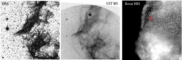
Figure 1. (Left) Optical (red) image of the eastern portion of the Cygnus Loop containing the star KPD 2055+3111 (indicated by cross hairs), from the DSS. (Center) The same region from the UIT B5 filter image near 1500 Å. KPD 2055+3111 is the brightest stellar feature in the image. (Right) ROSAT HRI image of the region, with a circle indicating the position of the star. north is up and east is to the left. The region shown is approximately 20' on a side.
Download figure:
Standard image High-resolution image2.2. FUSE Specifics and Data Reductions
We used the FUSE satellite to observe both KPD 2055+3111 and adjacent regions of nebular emission. The FUSE satellite was launched on 1999 June 24, began nominal science observations in 1999 December and ceased science operations in 2007 October. The characteristics and capabilities of FUSE have been described in detail by Moos et al. (2000), Sahnow et al. (2000a, 2000b), and Moos et al. (2002). The FUSE instrument consisted of four primary mirrors, each with its own separate focal plane and grating. Each of these optical paths is called a "channel." Two of the primary mirrors (and their gratings) were coated with LiF and aluminum, optimizing them for the longer wavelength end of the FUSE range, and the other two channels used SiC, optimized for the shorter wavelengths.7 The FUV spectra formed by these channels were focused onto two microchannel plate intensified wedge and strip detectors, each with two segments, A and B. FUSE operated over the wavelength range 905–1187 Å, with a nominal point source resolution R = λ/Δλ ⩾ 20, 000 (although somewhat variable with wavelength and spectrograph channel).
The FUSE observations are summarized in Table 1 and the aperture positions are shown in Figure 2, which shows a 4' region centered on the star. A preliminary observation from the FUSE Cycle 3 program C052 demonstrated feasibility, and a Cycle 4 program D049 provided the data of most interest for this paper. For these observations the 4'' × 20'' aperture (dubbed MDRS in FUSE nomenclature) was prime, and since the total expected count rates were low, the time-tag mode was used.
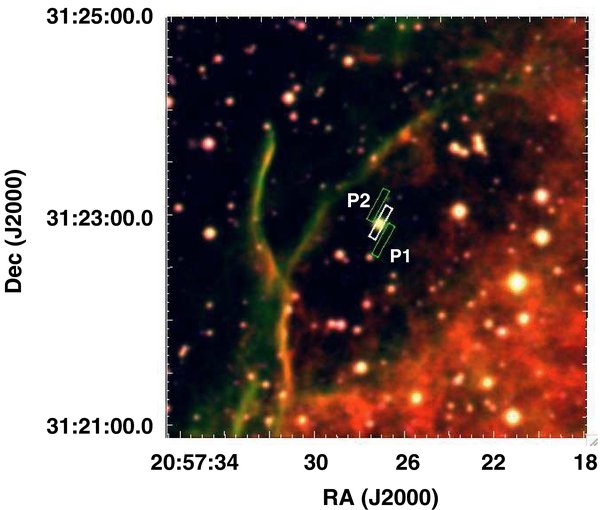
Figure 2. 4' square region around KPD 2055+3111, with the reconstructed FUSE aperture positions shown. The green boxes show FUSE MDRS apertures for the nebular spectra, with NGC6992-P1 to the southwest and P2 to the northeast. The white box is the MDRS aperture centered on KPD 2055+3111. The background image was constructed from the DSS, where red is the POSS2-red band (mainly Hα), green is the POSS2-blue data (mainly [O iii]λ5007), and the POSS2-IR band (which only shows stars) is displayed as blue. Hence, stars that appear in all three bands appear white.
Download figure:
Standard image High-resolution imageTable 1. Log of Observations
| Target Obs ID | Coordinates (J2000) | Aperture Position Angle | Date (UT) | Integration Time (ks) |
|---|---|---|---|---|
| KPD 2055+3111 | 20:57:26.85 | MDRSa | 2002 Jul 7 | 2.2 |
| C0520101 | +31:22:53.0 | 303° | ||
| KPD 2055+3111 | 20:57:26.85 | MDRSa | 2003 Nov 26 | 16.7 |
| D0490101 | +31:22:53.0 | 151° | ||
| NGC6992-P1 | 20:57:26.75 | MDRSa | 2003 Nov 25 | 8.3 |
| D0490102 | +31:22:43.0 | 150° | ||
| NGC6992-P2 | 20:57:26.95 | MDRSa | 2003 Nov 25 | 4.0 |
| D04901003 | +31:23:03.0 | 150° | ||
| KPD 2055+3111 | 20:57:26.85 | 1''×300'' | 2002 Sep 16 | 2.7 |
| MDM-2.4m Optical | +31:22:53.0 | 90° |
Note. aData through three FUSE apertures obtained simultaneously, with the 4'' × 20'' MDRS aperture being prime; see text.
Download table as: ASCIITypeset image
Because of small thermal drifts, the relative alignment of the four channels was not completely stable. Channel alignment varied in an approximately repeatable way as the FUSE boresight was moved from one part of the sky to another, but there were also motions of 3–6'' on orbital (∼100 minutes) timescales. This was not a significant problem for point sources when the LWRS (30'' square) aperture was primary, because the motions were a small fraction of the aperture size. However, the MDRS apertures were only 4'' wide, meaning that alignment on a stellar source was approximate at best. Since the LiF1 channel was used for guiding for the data reported here, this channel was pointed with sub-arcsec accuracy while the other channels drifted in and out of alignment. Thus, we concentrate on the data from this channel, especially for the stellar sight line.
FUSE data for all of the apertures and observations were processed with a standardized software pipeline, with the data presented here being from CalFUSE version 2.4. For the stellar spectrum (D04901) individual exposures were co-aligned by channel and segment before summing using the IDL routine fuse_register.8 Figure 3 provides an overview of the resulting LiF1 channel data (995–1185 Å). The FUV continuum falls slowly from 1.2 × 10⁻¹² to 0.5 × 10⁻¹² erg cm−2 s−1 Å−1 across the FUSE range, and numerous narrow photospheric and interstellar lines are present. A narrow spike at 1025.6 Å is the Lyβ airglow line in the center of the broad stellar absorption in this line. We note that, due to astigmatism in the optical system perpendicular to the dispersion, no spatial information is available within the individual FUSE apertures.
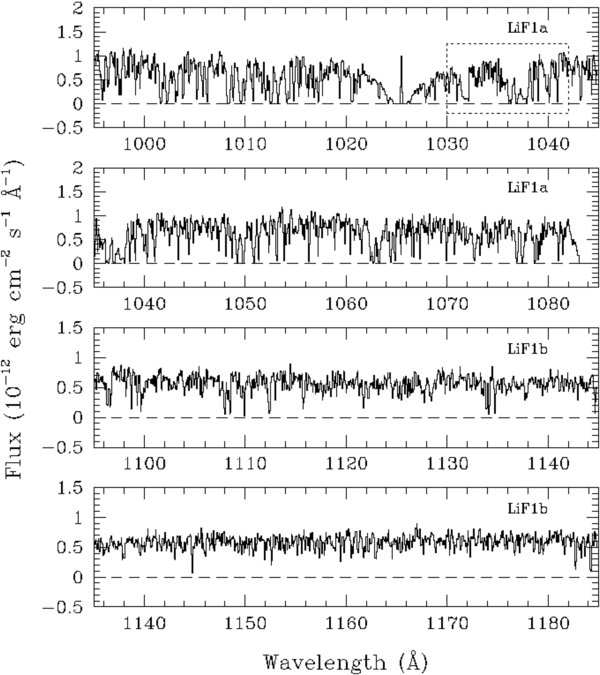
Figure 3. Overview of the FUSE spectrum of KPD 2055+3111 from 995 Å to 1185 Å. The dashed box in the top panel shows the region enlarged in Figure 7.
Download figure:
Standard image High-resolution image
Figure 4. Extracted O vi emission line profiles from the LiF1A MDRS spectra adjacent to the KPD2055+3111 sight line, shown on a velocity scale. The top two panels are λλ1032, 1038 from NGC6992-P1 (southwest) and the bottom two panels are the same lines from NGC6992-P2 (northeast). Note the dramatically different structural details in the emission profiles from these two positions, only separated by ∼20''.
Download figure:
Standard image High-resolution imageThe MDRS emission region aperture positions were selected to be as close as possible to KPD 2055+3111, while also being far enough away to avoid the star as the channels drifted. These positions were chosen to be just southwest (NGC6992-P1) and northeast (NGC6992-P2) of the star, or roughly perpendicular to the long dimension of the apertures (see Figure 2 and Table 1). As with the stellar spectrum, the individual exposures at each position were aligned and summed, although the alignment in these data were accomplished using the Lyβ airglow line for reference.
While the emission-line positions (and the star itself) appear to sit in a "hole" in the optical emission (see Figures 1 and 2), previous work in the Cygnus Loop (Blair et al. 2002) led us to suspect that the FUV emission would be present at the observed positions. This suspicion was correct. Strong emission in O viλλ1031.9138, 1037.6154,9 was detected at both offset positions. The O vi lines from the resulting spectra are shown on a velocity scale in Figure 4. Here and elsewhere in this paper, velocities are shown corrected to the local standard of rest (LSR) system. By selecting emission regions on either side of the star, we hoped to sample any gradient in the emission properties on small scales, and average them to obtain the best estimate of the emission properties directly on the stellar sight line. This could then be compared to the stellar O vi absorption profile.
However, while there is little change in the overall O vi line intensities over these small angular distances, the details of the line profiles show significant variability between the two spectra. This was not expected, and it impacts our ability to intercompare the emission and absorption line data. The overall extent of emission in O vi λ1032 covers roughly 300 km s−1, from −200 to slightly over +100 km s−1. The P2 data (northwest of the star) shows significantly more structure in the line profile than for P1. The possible reasons for this are discussed in Section 3.4.
2.3. Optical Spectral Data
New optical spectra of KPD 2055+3111 were kindly obtained for us by Robert Fesen (Dartmouth), using the OSU Boller and Chivens CCD spectrograph on the 2.4 m Hiltner Telescope at the MDM Observatory in Arizona. Details are provided in Table 1. The spectrum covered the 3500–7000 Å region with 7 Å resolution, which is ideal for model fitting of sdO, sdOB, and sdB stars (e.g., Saffer et al. 1997). These data were reduced by us using standard procedures within IRAF,10 including the use of flux calibration standard stars to obtain flux calibrated spectra of the star. The reduced, normalized spectrum, covering the 3800–5000 Å region of most interest to the models fits, is shown in Figure 5. The spectrum shows strong Balmer lines, the He i λ4026, λ4388, λ4471, λ4713, and λ4922 lines, and the He ii λ4686 line.
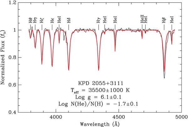
Figure 5. Normalized portion of our optical spectrum of KPD 2055+111. The smooth red line represents the best fit model of the optical spectrum. The atmospheric parameters for this fit are indicated.
Download figure:
Standard image High-resolution imageThe original sdO designation for KPD 2055+3111 arose from the presence of He ii lines comparable to the Balmer lines in low resolution optical spectra by Downes (1986). However, our optical spectrum shows several He i lines in addition to the Balmer lines and He ii λ4686 line, and hence it is more appropriate to classify it as an sdOB star. Spectral model fits are provided in the following section.
3. ANALYSIS AND DISCUSSION
3.1. Stellar Modeling and Derivation of Parameters
We fitted the optical spectrum of KPD 2055+3111 with a grid of stellar atmosphere models computed with the programs TLUSTY and SYNSPEC (Hubeny & Lanz 1995). The grid consists of non-LTE models with various values of effective temperature 20,000 K ⩽Teff ⩽ 80,000 K in steps of 2000 K, various values of gravity 4.8 ⩽ log g ⩽ 6.4 in steps of 0.2 dex, and various values of helium abundance −4.0 ⩽ log N(He)/N(H) ⩽ 0.0 in steps of 0.5 dex. The best atmospheric parameters are obtained by using a χ2 minimization technique based on the Marquardt method (see Bevington & Robinson 1992). Figure 5 shows the best fit of the optical spectrum of KPD 2055+3111 and the results are summarized in Table 2. The Hβ line was excluded from the fit because of an unexplained discrepancy on its red wing. We obtained Teff = 35,500 ± 1000 K, log g = 6.1 ± 0.1, and log N(He)/N(H) = −1.7 ± 0.1. Using the best parameters for KPD 2055+3111, we computed the intrinsic color index (B − V)0 that we compared to the observed (B − V) in order to estimate the amount of reddening in its direction. We obtained (B − V)0 = −0.27 by using the passbands of Bessell (1990). The extinction in the direction of KPD 2055+3111 is then just E(B − V) = (B − V) − (B − V)0 = 0.03 ± 0.01.
Table 2. Measured and Derived Parameters for KPD 2055+3111
| Parameter | Value | Reference |
|---|---|---|
| Spectral type | sdOB | 2 |
| V | 14.12 | 1 |
| (B − V)obs | −0.24 | 1 |
| Teff (K) | 35,500 ± 1000 | 2 |
| log g | 6.1 ± 0.1 | 2 |
| log [N(He)/N(H)] | −1.7 ± 0.1 | 2 |
| (B − V)0 | −0.27 | 2 |
| E(B − V) | 0.03 ± 0.01 | 2 |
| Distance (pc) | 576 ± 61 | 2 |
References. (1) Downes (1986); (2) This paper.
Download table as: ASCIITypeset image
This extinction is lower than the value of E(B − V) = 0.08 often quoted for the Cygnus Loop, which is in the foreground of KPD 2055+3111. However, a careful assessment of previous work on the emission filaments shows this value can easily be accommodated. Color excess determinations for the emission filaments are dependent on assumptions about the intrinsic Balmer decrement and the extent to which collisional processes may affect it. Fesen et al. (1982) observed 14 radiative filaments throughout the Cygnus Loop structure. None were particularly close to KPD 2055+3111, but assuming an intrinsic Hα:Hβ ratio of 3.0 (i.e., a small amount of collisional excitation above case B recombination), the range of E(B−V) observed for these positions is consistent with zero (or at least very little) extinction on some sight lines and up to E(B−V) ≈ 0.3 on other sight lines. Apparently the sight line toward KPD 2055+3111 has relatively low extinction.
We can estimate the evolutionary status of KPD 2055+3111 by comparing its position in a log g–Teff diagram to evolutionary tracks of post-extreme horizontal branch (post-EHB) stars. Figure 6 compares the position of KPD 2055+3111 and field sdB stars to evolutionary tracks computed by Charpinet et al. (2000, 2002). The evolutionary tracks are computed for models that start from the zero-age extended horizontal branch (ZAEHB) and evolve toward the white dwarf region as low mass white dwarf stars. Numbers along the tracks indicate the mass of the star in solar units. The models with 0.4760 M☉, 0.4770 M☉, 0.4780 M☉, 0.4790 M☉, and 0.4800 M☉ have a core mass Mc = 0.4758M☉, while models with 0.4691 M☉ and 0.4697 M☉ have Mc = 0.4690 M☉. As pointed out by Dorman et al. (1993), one of the most important parameters that governs the evolution of post-EHB stars is the hydrogen envelope mass Menv that surrounds the helium-burning core. The models in Figure 6 have, respectively, from left to right, Menv = 0.0001 M☉, 0.0002 M☉, 0.0007 M☉, 0.0012 M☉, 0.0022 M☉, 0.0032 M☉, and 0.0042 M☉. In each case, Menv is too small to ignite the hydrogen-burning shell, and therefore, the evolutionary models predict that the star must be hot, compact, and subluminous.
Figure 6. Position of KPD 2055+3111 in the log g–Teff plane, using our derived parameters. Post-EHB evolutionary tracks (continuous lines) computed by Charpinet et al. (2000, 2002) are shown. Each evolutionary track is labeled by the mass of the star in solar mass units. The open circles are the positions of field sdB stars.
Download figure:
Standard image High-resolution imageThe stellar parameters derived from the optical data were used to construct a detailed model atmosphere calculation to fit to the FUV spectrum. The resulting model is shown in Figure 7, overlaid on a section of the FUSE spectrum. This model does a good job of approximating many, but not all, of the narrow photospheric lines in the spectrum. Indeed, this is the best that can be done at present. For stars in this temperature range, three and four times ionized atoms dominate the ionization balance in the photosphere. Unfortunately, the atomic data of these ionization states for the iron peak elements are practically nonexistent in the FUSE band. Hence, we cannot obtain a perfect stellar model that reproduces all of the observed stellar lines. As Figure 7 shows, the spectrum also contains numerous H2 and other IS absorption lines as well.
Figure 7. 10 Å region of the FUSE spectrum of KPD 2055+3111 near the O vi lines. The solid line is the FUSE data and the dotted line is a stellar model spectrum that roughly matches many of the photospheric lines, which are identified at the top of the plot. The broad absorptions near 1032 and 1038 Å are due to O vi from the SNR (see Figures 10 and 11). Broad absorptions due to IS C ii λ1036.7 and narrower absorptions due to H2 and other ISM lines are also evident, as indicated at the bottom of the plot.
Download figure:
Standard image High-resolution image3.2. H2 Absorption
H2 absorption is clearly present on the sight line, but deriving its properties is significantly complicated by the complexity of the intrinsic stellar spectrum. Thus we first performed an assessment of the features present in the D0490101 LiF1A and LiF1B spectra to determine the best lines for use in the analysis of H2 column densities. The stellar model discussed above was a key element in identifying the cleanest H2 lines to use for this analysis especially in the LiF1A data segment. Once the best lines were identified, the model column densities for lines within each observed rotational level were found via a profile-fitting technique that included the effects of the stellar spectrum on the continuum. This procedure is described in more detail below.
To identify the lines of interest, assess their utility, and ultimately find the H2 column densities, we utilized the H2OOLS modeling code of McCandliss (2003). Overplotting an H2OOLS template file convinced us that only lines from the V = 0 vibrational level were clearly present, and the rotational levels 0 ⩽ J ⩽ 5 were identified. Preliminary line width measurements were used to identify potentially blended features and help identify the cleanest lines from each J-level. Once the best reference lines for each J-level were established, additional lines for each level were identified for use in consistency checks of the column densities derived from the reference lines. A total of 73 lines were used to find the column densities for the individual J levels.
Column densities for each J level were found with the following procedure. An H2OOLS template for a particular b value and vibrational level (V = 0 in our case) were read into IDL, which contained arrays for H2 template wavelengths and optical depths for each potential line. H2OOLS provides templates for b-values ranging from 1 to 20 km s−1 in integral steps and uses atomic data from Abgrall et al. (1993a, 1993b). A value for N(H2)J was defined, then multiplied with the template optical depth, creating a normalized model. The template wavelengths were interpolated and aligned with the spectrum wavelength array to create a model wavelength vector that matched the data. A small grid of such models, compared against the reference lines for each J level bounded the appropriate column density range, and then an iterative procedure arrived at a best fit to the b value and column for the reference lines. In all cases b = 12 km s−1 provided the best fits. This best fit model was then compared against the secondary lines to verify consistency. After fitting each J level separately, the models were then combined into a single H2 model representing the H2 spectrum on this sight line. In Figure 8, we show a small data section with this final model overlaid. The N(H2)J values derived are summarized in Table 3. The total column density in H2 for J = 0–5 is (3.3 ± 0.6) × 1016 cm−2.
Figure 8. Best fitting H2 model is overlaid on FUSE data sections. Vertical lines identify several of the primary reference lines described in the text.
Download figure:
Standard image High-resolution imageTable 3. H2 Model Column Densities
| J | gJ | Number of Lines | NJ (×1015 cm−2) | log NJ (cm−2) |
|---|---|---|---|---|
| 0 | 1 | 5 | 8.0 ± 3.0 | 15.90+0.14−0.20 |
| 1 | 9 | 13 | 14.5 ± 5.5 | 16.16+0.14−0.21 |
| 2 | 5 | 14 | 3.6 ± 0.1 | 15.55 ± 0.006 |
| 3 | 21 | 14 | 3.5 ± 1.1 | 15.54+0.12−0.16 |
| 4 | 9 | 13 | 1.3 ± 0.1 | 15.10 ± 0.02 |
| 5 | 33 | 14 | 1.7 ± 0.4 | 15.23+0.09−0.12 |
Download table as: ASCIITypeset image
With the column densities determined, the excitation temperature of the molecular hydrogen can be derived, as described in Section 3.2 of Graham et al. (1991a). In Figure 9, we show a plot of  where gJ is the statistical weight for that J, versus the excitation potential. The data exhibit unique slopes for 0 ⩽ J ⩽ 1 and 2 ⩽ J ⩽ 5. The slope m of the line of best fit was determined in both of these regions, and temperature was derived using the relation
where again m is the slope. We find T(J = 0–1) = 106 ± 40 K and T(J = 2–5) = 850 ± 230 K.
Figure 9. Derived H2 column densities as a function of J-level are shown. The error bars at J = 3 and 5 are smaller than the symbols (see text).
Download figure:
Standard image High-resolution image
Figure 10. (a) (Top) MDRS spectrum of KPD 2055+3111 in the O vi region is shown in the top curve, and the emission region spectra are overplotted at the bottom, on the same vertical scale. (b) The corrected KPD 2055+3111 spectrum is shown after subtracting the average emission component. The heavy line shows the best two component fit to the O vi absorption lines (see text).
Download figure:
Standard image High-resolution imageThis two-temperature result is consistent with H2 observed on other interstellar sight lines (e.g., Spitzer & Cochran 1973; Savage et al. 1977) and hence is consistent with an ISM origin. Although the temperature for the higher J levels is somewhat high, it is still within the range observed elsewhere in the ISM. We find no evidence from either the width of the reference lines, component structure, or relative displacements of higher J-level lines relative to lower J-level lines, that any significant portion of the H2 observed is directly associated with the Cygnus Loop shocks. This is somewhat surprising given that shocked H2 has been identified at several locations in the Cygnus Loop using infrared (IR) observations (Graham et al. 1991a, 1991b). However, the H2 identified by Graham et al., which had excitation temperatures of 2200 ± 500 K, was associated with magnetic shock precursor heating at positions on the outer limb of the Cygnus Loop nonradiative shocks. The absence of any indication of H2 with similar characteristics on the sight line to KPD 2055+3111 indicates either that this mechanism only operates for the outer nonradiative shocks, or that the H2 excitation via this mechanism is patchy.
3.3. O vi Absorption from the Cygnus Loop
In order to measure the O vi absorption, we first correct the stellar spectrum for overlying O vi emission, as seen in the MDRS emission spectra. Since FUV emission apparently covers the entire region, the O vi emission entering the aperture at the stellar position prevents the O vi absorption from decreasing all the way to zero, as can be seen at ∼1032 Å in Figure 7. To remove the emission contamination from the stellar aperture position, we have followed a simple procedure of averaging the two emission positions together and subtracting this from the spectrum of the star to obtain a corrected stellar spectrum. In Figure 10(a), we show the average emission spectrum overlaid on the extracted stellar spectrum, and in Figure 10(b) we show the corrected spectrum. Despite the variations in the line profiles as indicated in Figure 4, this procedure has worked quite well in correcting the stellar spectrum O vi profiles to zero. Figure 10(b) also shows an overlay of the O vi absorption model described below.
O vi column density measurements were performed using the profile-fitting routine FSIM, originally written to produce accurate simulated spectra for FUSE. An emission-subtracted spectrum of KPD 2055+3111 was read into FSIM, along with the best fitting H2 model and the calculated stellar model scaled to the data. Thus, only the SNR and ISM absorption lines produced large divergences from the initial model. We then added Gaussian absorption components, concentrating on the λ1032 line which suffers the least complications. Because of the substantial H2 column found above, the H2 model shows that several H2 lines overlap or lie in close proximity to the O vi lines: the λ1032 feature was contaminated by H2 at 1032.356 Å (R(4)) on the red wing, while the λ1038 feature was contaminated at 1038.156 Å (P(1)) and 1037.146 Å (R(1)).
Figure 11 shows the model fit near O vi λ1032, where the data have been plotted on a velocity scale. The FSIM analysis revealed the need for two O vi components, the parameters of which are shown in Table 4. There is an average velocity difference between the O vi components of Δv ≈ 100 km s−1. The opposite velocities of the two components relative to the rest wavelength probably indicates that the sight line is passing through a curved structure, with the foreground (blueshifted) component of lower column density than the background (redshifted) component.
Figure 11. Corrected O vi absorption region spectrum is shown on a velocity scale. The dashed line shows the best fitting stellar model (continuum component only) with H2 absorption plus a two-component model of the O vi absorption due to the Cygnus Loop. Vertical lines mark the fitted centroids of the two O vi components as shown in Table 4. Note that an H2 line also affects the red wing of the red O vi component. See Figure 7.
Download figure:
Standard image High-resolution imageTable 4. O vi Model Parameters
| Component | N(O5+) (cm−2) | b (km s−1) | v (km s−1)a |
|---|---|---|---|
| 1 | 1.87 × 10¹⁵ | 84 | +30 |
| 2 | 0.47 × 10¹⁵ | 82 | −75 |
Download table as: ASCIITypeset image
3.4. The Emission Spectra
The integrated fluxes in each O vi line were measured using an interactive IDL routine that simply fit a linear background locally around the line and summed the flux between limits marked by a cursor. The fluxes at each position are converted into surface brightnesses (flux per square arcsec) by dividing by the aperture area (assuming a filled aperture). O vi line fluxes and surface brightness determinations are listed in Table 5.
Table 5. O vi Emission Measurements
| Data Set | Aperture | F(λ1032)a | F(λ1038)a | Σ(λ1032)b | Σ(λ1038)b |
|---|---|---|---|---|---|
| D0490201 | MDRS | 0.55 | 0.32 | 6.83 | 3.97 |
| (NGC6992-P1) | |||||
| D0490301 | MDRS | 0.69 | 0.32 | 8.65 | 4.06 |
| (NGC6992-P2) |
Notes. aUnits of 10−13 erg cm−2 s−1. bUnits of 10−16 erg cm−2 s−1 arcsec−2.
Download table as: ASCIITypeset image
The surface brightnesses of O vi in the MDRS apertures at positions NGC6992-P1 and P2 are only lower than the bright regions in the Cygnus Loop by a factor of ∼3, despite almost nonexistent optical emission. This is in keeping with the discussion reported by Blair et al. (2002), who found the O vi intensities could be significant even where the optical emission was weak (for other locations in the Cygnus Loop). At face value, the surface brightnesses in O vi are also slightly lower than the intensity observed from the 180 km s−1 nonradiative shock in the NE Cygnus Loop reported by Sankrit & Blair (2002), and are most similar to those observed at the faster (400 km s−1) nonradiative shock at Cygnus Loop "P7" (Raymond et al. 2003).
The complexity and variability of the O vi line profiles in Figure 4 is interesting in its own right. This could be due to either spatial changes in the overlying absorption, or to variations in the complexity of the filaments encountered along the different sight lines. In principle, the components might also be due to thermal instabilities as described by Innes et al. (1987) and Innes (1992). With existing data, there is no clear way to choose between these options. However, we note that the region appears to be near the edge of a local X-ray enhancement in Figure 1 (right). The O vi line profiles, centered near zero velocity, show that we are observing the shock front close to edge-on. It has been shown that shocks around the perimeter of the Cygnus Loop have a "wavy-sheet" morphology (Hester 1987). The multiple (and variable) components in the O vi 1032 profiles suggest that these lines of sight intersect several tangential shock interfaces along this sheet of emission, and that the details are different for the two sight lines.
The ratio of the O vi doublet lines can be used to assess the optical depth in O vi. A ratio of two is expected in optically thin conditions, while a lower ratio is obtained with increasing optical depth. In Figure 12, we show plots of the λ1032/λ1038 ratio for the two emission line data sets, as a function of velocity. The overall flux ratio between the two components is about 2 or slightly lower across most of the line profiles, indicating the likely presence of some resonance line scattering. The ratios above 2, especially on the negative velocity side, are due to excess absorption of the λ1038 line, probably by strong, broad C ii λ1037.02, causing an artificially elevated ratio.
Figure 12. The O vi 1032/1038 ratio as a function of velocity for the two emission line regions. The data were binned to 0.15 Å to improve the signal-to-noise ratio per bin for taking ratios. Noisy values outside the line profile have been set to zero.
Download figure:
Standard image High-resolution image
Emission and absorption line measurements combined can provide unique diagnostics for shock properties (e.g., Raymond et al. 1991). However, the ability to exploit the combined results usually requires the assumption that the same parcel(s) of gas give rise to the emission and absorption. In the case of the shock front being discussed here, the edge-on geometry and the saturated O vi absorption line make it difficult to utilize the combined observations effectively. However, there is a feature in the P2 emission spectrum centered at −75 km s−1, which can reasonably be assumed to be associated with the absorption component at the same velocity, with an O vi column density of 4.7 × 1014 cm−2 (Table 4). If we make the further assumption that both the emission and absorption components arise in a single shock front, then we can compare observations to model predictions and derive the shock conditions. We fit the −75 km s−1 emission feature in the P2 spectrum with a Gaussian, yielding a flux of 3 × 10⁻¹⁴ erg cm−2 s−1, corresponding to a surface brightness of 3.75 × 10⁻¹⁶ erg cm−2 s−1 arcsec−2. The correction for interstellar extinction, with E(B − V) = 0.03 and using the reddening curve of Fitzpatrick & Massa (1999) is a factor of about 1.4, yielding an intrinsic surface brightness of about 5.3 × 10⁻¹⁶ erg cm−2 s−1 arcsec−2.
For a given shock velocity, the column through a complete O vi zone is independent of the preshock density. The flux, however, is proportional to the preshock density. A third constraint for the Cygnus Loop is that the age of the shock has to be less than the age of the remnant (∼5000 years), and so the O vi zone needs to be formed and completed within that time.
We find that the observations are reproduced by a 180–200 km s−1 shock moving into gas with a hydrogen number density nH ∼ 0.75 cm−3. The observed velocity of the shock, −75 km s−1 implies that the shock normal makes an angle of about 65° to the line of sight. The O vi zone is complete by the time about 1.5 × 1018 cm−2 of hydrogen has been swept up, corresponding to an age of about 3000 years. The measured O vi column is reproduced correctly (taking into account the inclination angle). The O vi λ1032 surface brightness is predicted to be about 1.5 × 10⁻¹⁵ erg cm−2 s−1 arcsec−2, which is somewhat higher than the reddening corrected value measured. This discrepancy could be at least partially explained by resonance line scattering of the O vi line as mentioned above, which would reduce the observed intensity from its intrinsic value.
We note that the measured brightness of this −75 km s−1 component is significantly higher than can be produced by single shocks with velocities above about 200 km s−1 unless the preshock density is of order 5 cm−3, or unless the shock age is longer than about 104 years, neither of which is likely for the Cygnus Loop (e.g., Sankrit & Blair 2002, Raymond et al. 2003).
3.5. The Distance to KPD 2055+3111
The position of KPD 2055+3111 in the log g–Teff diagram indicates that it is still on the EHB and that its mass is around 0.47 M☉. A star on the EHB burns helium in its core for about 108 yr, and then, without reaching the asymptotic giant branch, evolves rapidly toward the white dwarf region for about 107 yr. By assuming a mass of 0.47 M☉ for KPD 2055+3111 and using the observed gravity (log g = 6.1), we can estimate its radius, and then its distance by using the relation
where Fobs is the observed flux at the earth, F is the emergent flux at the surface of the star, R is the radius of the star, and D is the distance to the star. Equation (2) can be rearranged by expressing Fobs as a function of the V magnitude, and by taking into account the interstellar absorption AV along the line of sight of KPD 2055+3111; therefore the distance becomes
where G is the gravitational constant, M is the mass of the star in grams, HV is the Eddington flux from the model atmosphere weighted by the Johnson passband V provided by Bessell (1990), g is the gravitational acceleration, and F0,V is the average absolute flux of Vega at V as specified in Heber et al. (1984). By taking RV = 3.1 and E(B − V) = 0.03, the interstellar absorption is AV = 0.093. The distance to KPD 2055+3111 is then D = 576 ± 61 pc.
This result is an independent confirmation of the smaller distance for the Cygnus Loop as determined first by Blair et al. (1999) and then refined by Blair et al. (2005) from two epochs of Hubble Space Telescope (HST) WFPC2 imaging. The current best value from that analysis (540 [+100, −80] pc) indicates that KPD 2055+3111 is only slightly more distant than the Cygnus Loop itself. Our nominal best fitting distance constrains the upper limit allowed from the HST analysis.
4. SUMMARY
We have presented FUSE and optical observations of KPD 2055+3111, a sdOB star, and two adjacent FUSE sight lines that sample nearby emission from the NE Cygnus Loop SNR. O vi absorption due to the Cygnus Loop is clearly seen against the spectrum of the star, proving the star is indeed behind the SNR. This is the first and only UV background star that has been identified for the Cygnus Loop. The O vi absorption can be fit successfully with a simple two-component model, with the components overlapping but separated by ∼100 km s−1.
Molecular hydrogen lines are also seen against the star's spectrum. An analysis of this absorption is consistent with an interstellar origin, although some contribution from the SNR cannot be ruled out. However, any SNR H2 on this sight line is considerably different from that detected by Graham et al. (1991a, 1991b) on the outer limb of the SNR and attributed to a magnetic shock precursors.
Strong O vi emission is detected in both adjacent positions observed with FUSE, despite a near total lack of optical emission. Surprising variations in the line profiles are seen between these two positions, which were centered only ∼20'' apart on either side of KPD 2055+3111. We cannot unequivocally attribute these variations to a particular cause, although the general morphology of various emissions makes it reasonable to assume the two positions are sampling varying (but optically invisible) line-of-sight shock structures. Unfortunately, the complexity seen in the emission line profiles impacts our ability to make a meaningful comparison of the emission and absorption components.
Model fits to the stellar spectrum allow its characteristics to be determined, and its distance to be calculated as 576 ± 61 pc, which places an independent upper limit on the distance to the Cygnus Loop. This value is consistent with the proper motion distance to the Cygnus Loop reported by Blair et al. (2005) of 540 [+100, −80] pc, and modestly constrains the upper limit.
It is a pleasure to thank the FUSE operations team at JHU for their efforts in obtaining these data. We also thank Robert Fesen for obtaining the new optical data on KPD 2055+3111. This work has been supported by NASA grants NAG5-12423, NNG04GJ25G, and NNG05GD75G, all to the Johns Hopkins University.
Footnotes
- *
Based on observations made with the NASA-CNES-CSA Far Ultraviolet Spectroscopic Explorer (FUSE). FUSE was operated for NASA by the Johns Hopkins University under NASA Contract NAS5-32985.
- 6
This research has made use of the SIMBAD database, operated at CDS, Strasbourg, France.
- 7
- 8
- 9
For convenience, we will sometimes refer to these lines in the text with abbreviated wavelength notation, viz., λλ1032, 1038.
- 10
IRAF is distributed by the National Optical Astronomy Observatories, which are operated by the Association of Universities for Research in Astronomy, Inc. (AURA) under cooperative agreement with the National Science Foundation.