


ABSTRACT
We analyze stellar convection with the aid of three-dimensional (3D) hydrodynamic simulations, introducing the turbulent cascade into our theoretical analysis. We devise closures of the Reynolds-decomposed mean field equations by simple physical modeling of the simulations (we relate temperature and density fluctuations via coefficients); the procedure (Convection Algorithm Based on Simulations) is terrestrially testable and is amenable to systematic improvement. We develop a turbulent kinetic energy equation which contains both nonlocal and time-dependent terms, and is appropriate if the convective transit time is shorter than the evolutionary timescale. The interpretation of mixing-length theory (MLT) as generally used in astrophysics is incorrect; MLT forces the mixing length to be an imposed constant. Direct tests show that the damping associated with the flow is that suggested by Kolmogorov (εK ≈ ρ(u')3rms/ℓD, where ℓD is the size of the largest eddy and (u')rms is the local rms turbulent velocity). This eddy size is approximately the depth of the convection zone ℓCZ in our simulations, and corresponds in some respects to the mixing length of MLT. New terms involving the local heating due to turbulent dissipation should appear in the stellar evolutionary equations, and are not guaranteed to be negligible. The enthalpy flux (stellar "convective luminosity") is directly connected to the buoyant acceleration, and hence to the scale of convective velocity. MLT tends to systematically underestimate the velocity scale, which affects estimates of chromospheric and coronal heating, mass loss, and wave generation. Quantitative comparison with a variety of 3D simulations reveals a previously unrecognized consistency. Extension of this approach to deal with rotational shear and MHD is indicated. Examples of application to stellar evolution will be presented in subsequent papers in this series.
Export citation and abstract BibTeX RIS
1. INTRODUCTION
More than 50 years ago, the version of the "mixing-length theory" (MLT) of convection, which became the preferred basis for the subsequent study of stellar evolution was introduced (Biermann 1951; Vitense 1953; Böhm-Vitense 1958). Despite much effort (still ongoing), MLT is still the standard choice for the field.
In this paper we develop a new procedure, "Convective Algorithms Based on Simulations" (CABS), in which we close the Reynolds-decomposed, angular, and time-averaged equations by simple physical models based upon analysis of fully three-dimensional (3D), time-dependent turbulent stellar convection (Meakin & Arnett 2007b). These simulations include convective boundaries within the computational volume (as far from the edges of the grid as feasible), and allow interface physics to be examined. The resulting theoretical formalism allows us to incorporate content from other simulations (especially Chan & Sofia 1989, 1996; Kim et al. 1995, 1996; Porter & Woodward 2000; Porter et al. 2000; Robinson et al. 2004), and from research in other fields, such as terrestrial fluids (Turner 1973), oceanography (Gill 1982), and meteorology (Dutton 1986), which have a firmer empirical basis. We develop a simple description of the convective velocity field as seen in our simulations. This effort brings some startling suggestions for revision of our interpretation of MLT, and suggests how our approach may be generalized to include rotation and magnetic fields (Balbus & Hawley 1998; Pessah et al. 2006). This is timely, considering recent success in simulating turbulent plasma with magnetic fields (Browning 2008; Schüssler & Völger 2008).
Since the formulation of MLT, there has been a considerable development in understanding the nature of chaotic behavior in nonlinear systems; see Cvitanović (1989) for a review and reprints of original papers, and Frisch (1995), Gleick (1987), Thompson & Steward (1986). Lorenz (1963) presented a solution to the Rayleigh problem of thermal convection (Chandrasekhar 1961b) which captured the seed of chaos in the Lorenz attractor, and contains a representation of the fluctuating aspect of turbulence not present in MLT. Kolmogorov (1962) and Obukhov (1962) developed the modern version of the turbulent cascade. Although already formulated, the original theory (Kolmogorov 1941) was not used in MLT.
We derive our approximate theory from a consideration of the full equations of 3D compressible hydrodynamics for a multiple-component fluid. These are close to the corresponding equations for a high beta (matter-dominated) plasma. This approach will allow us to incorporate a variety of phenomena in a coherent way, and to evaluate their relative importance, rather than to patch together various bits of physics piecemeal. Here we focus on the dominant features of nonrotating, nonmagnetic, turbulent, compressible fluid flow. The results are applicable to almost all stages of stellar evolution (any stage having convection or shear).5
In Section 2, we examine the physical aspects of stellar convection, and show that the velocity scale is set by the balance between buoyant driving and damping in the Kolmogorov cascade. Appropriate averaging allows us to deal with mild time dependence and reveals a robust underlying behavior. We develop a kinetic energy (KE) equation describing the average properties of turbulent convection, which shows how turbulent motion is created, transported, and destroyed. In Section 3, we incorporate this theoretical development into the equations of stellar evolution with turbulent convection, including new terms. Section 4 uses the theoretical development to compare our simulations to others, and finds previously unrecognized similarities. Section 5 indicates some important implications of this work, including how the effects of burning, rotation, and magnetic fields may be included. Section 6 summarizes our results and conclusions. Quantitative treatment of the dynamics of fluctuations and a comprehensive algorithm for stellar evolutionary calculations will be developed in subsequent papers in this series.
2. PHYSICAL ASPECTS OF STELLAR CONVECTION
Stellar convection has high Reynolds numbers because of the large linear scales, and is therefore highly turbulent. Our simulations have adequate resolution to show this type of behavior. Turbulent convection has several key features that need to be modeled: (1) it is nonlocal, (2) it has strong fluctuations in both space and time, (3) it is damped by a cascade of unstable vortices down to scales small enough for microscopic processes to dissipate effectively, (4) mixing of passive scalar properties is efficient, (5) turbulent behavior spreads to fill the volume allowed, and (6) buoyant acceleration is closely related to convective (enthalpy) flux, so that convective KE is closely tied to convective luminosity. MLT incorporates (4) and imperfectly deals with (6); we will address all six issues.
Cattaneo et al. (1991) found that 3D simulations of turbulent convection had two aspects: (1) vigorous, large-scale downflows,6 and (2) disorganized weaker motions. These two aspects have been confirmed by many other simulations, including our own. MLT attempts to describe the average properties of the disordered aspect. We will construct a theory which includes both; buoyant acceleration is characteristic of the largest scales, and turbulent dissipation of the smallest.
2.1. The Kinetic Energy Equation
We start with the equations we used in our 3D simulations (Meakin & Arnett 2007b). We use Reynolds decomposition of relevant flow and thermodynamic variables, which separates the fluctuating components from the slowly varying components (Tennekes & Lumley 1972). Numerical simulations dissipate features with wavelengths at or below the grid scale, and we will identify this with dissipation in the turbulent cascade (Kolmogorov 1941, 1962).
In the process of approximation of partial differential equations by finite methods, there is inevitably a loss of information at scales smaller than the grid size. A single volume element in space is approximated as a homogeneous entity; this is equivalent to complete mixing at this scale, at each time step, of mass, momentum, and energy. The loss of information that occurs with this mixing corresponds to an increase in entropy (Shannon 1948); the mixing of momentum is equivalent to the action of viscosity (Landau & Lifshitz 1959). In 3D flow, turbulent energy will cascade from large scales to small, at a rate set by the largest scales. We use an implicit subgrid dissipation in our large eddy simulation (ILES), which is the most computationally efficient way to deal with turbulent systems with a large range of scales (Boris 2007; Woodward 2007); the largest scales, which set the rate of cascade and contain most of the energy, are resolved on our grid and explicitly calculated, while the subgrid scales are dissipated in a way consistent with the Kolmogorov cascade.
Sytine et al. (2000) demonstrated that the piecewise parabolic method (PPM) based on the Euler equation (which has no explicit viscosity) converges to the same limit as methods based on compressible viscous equations (which do have explicit viscosity), as the grid is refined to smaller zones and smaller effective viscosity (the relevant limit for astrophysics). Porter et al. (2000) show the compatibility of mildly compressible flow with the Kolmogorov (1941) spectrum; Kritsuk et al. (2007) have pushed this to highly compressible flows as well. To represent the subgrid dissipation, which is inherent in our simulations, we explicitly introduce a volumetric dissipation rate for KE, εK, in our theoretical analysis. However, the turbulent cascade is a property of the whole convective flow, so connection to turbulence theory must be made through integrals of εK over the convection zone. Note that this is different from defining εK as a function of local variables (e.g., Smagorinsky 1963; Chan & Sofia 1989; Hansen & Kawaler 1994; Asida & Arnett 2000); see below.
The KE equation for convective motion was given in Meakin & Arnett (2007b). Taking the scalar product of the velocity with the equation of motion, we decompose the convective velocity u, the density ρ, and the pressure p into mean and fluctuating components (e.g., p = p0 + p'), so the time averages are  and
and  . This choice of just u, p, and ρ for this Reynolds decomposition into average and fluctuating parts gives the simplest equation for KE; the velocity u is derived from buoyancy and pressure forces (ρ and p fluctuations).
Using the hydrostatic equilibrium condition, and performing averages, gives (see Equation (A12) in Meakin & Arnett 2007b),
We use 〈p〉 to denote an average over angles at constant radius. The time average is taken over durations greater than a transit time ttransit = ℓCZ/(u')rms, where ℓCZ is the depth of the convective region, and (u')rms is the rms velocity across this region. This smooths the fluctuations, gives a nonlocal character to the analysis, and implies a separation of timescales into short (t ≪ ttransit) and long (t ≫ ttransit). We consider the case in which we may integrate over these short timescales and explicitly calculate the evolution on the long timescales.
Here EK is the KE per unit mass, ρ is the mass density, u0 is the nonfluctuating part of the fluid velocity vector and u' its fluctuating part, so
is the energy flux due to pressure perturbations carried by fluctuations (this pressure–velocity correlation flux reduces to the acoustic flux when considering sound waves (Landau & Lifshitz 1959, p. 251), and contains the energy flux due to internal gravity waves),

is the flux of KE carried by convective turbulent motion, g is the gravitational acceleration vector, and εK is the volumetric rate of dissipation implied by the turbulent cascade down to small scales.
2.2. Boundaries
The location of convective boundaries is a long-standing problem in stellar astrophysics. It has long been known that some sort of "convective overshooting" is necessary for models to match observations. This has been conceived as mixing of material beyond the convective boundary, often by "penetrative convection." This problem exists in part because the convective boundary has been inappropriately defined (Meakin & Arnett 2007b, especially Sections 4.1 and 7). The standard definition used in MLT defines the convective boundaries using the thermodynamic nablas, which essentially mark the onset and cessation of buoyant acceleration. One of the essential properties of convection is that turbulence fills the space available. A more appropriate criterion is one in which the stellar background is stiff enough to contain the turbulent convection, and therefore must account for the relative strength of the turbulent flow and the elastic stable layers.
We will define the convective zone as that region in which the stratification of the medium is unstable to turbulent mixing. This is evaluated with the "bulk Richardson number"
where Δb = ∫ΔrN2dr is the buoyancy jump across a layer of thickness Δr in the radial direction, N2 is the Brünt–Väisälä frequency, u is the rms velocity providing shear, and l is the scale length of the turbulence (essentially the size of the largest eddies). The precise definition of the thickness Δr is a topic that deserves further study; in several cases we have noticed that the rapid change in N2 near a boundary tends to make Δb insensitive to the exact value of Δr chosen for integration to obtain Δb.
In the linear limit of plane parallel flow, a region with Rig ≲ 0.25 has enough KE to overcome the stable stratification (Dutton 1986). Here Rig is the "gradient" Richardson number, and is a locally defined quantity, used in a linear stability analysis. The "bulk" Richardson number RiB is an inherently nonlinear quantity based on integration over an extended region. Since Rig,crit > 0, this allows for N2 > 0 as well. This formulation recognizes that layers that are thermodynamically stable (real roots to N2) can be hydrodynamically unstable when KE is input to the zone. The bulk Richardson criterion allows more mixing than predicted by the Ledoux criterion; the Schwarzschild criterion ignores compositional effects, and also predicts more mixing than Ledoux (see Kippenhahn & Weigert 1990; Hansen & Kawaler 1994).
Stable regions adjacent to the convective zone will become Richardson unstable periodically as shear builds up from adjacent turbulent motions and waves generated by convection, leading to entrainment of material at convective boundaries (Fernando 1991). The bulk Richardson number is not only an indicator of a convective boundary; it also determines the "rate" at which the boundary migrates through the Lagrangian mesh by mixing processes (Meakin & Arnett 2007b), and thus provides a "dynamic" boundary condition for the flow.
2.3. Averages
Our analysis is based primarily upon the numerical simulations of oxygen shell burning in a 23 M☉ star, but is found to be broadly applicable to other examples of stellar convection (such as convective envelopes, which are driven by the superadiabatic layer at the top rather than the nuclear burning shell at the bottom). Our convective zone has a depth of two pressure scale heights (see Meakin & Arnett 2007b for details).
Why do we need to do averaging? Figure 1 shows the behavior of the largest terms in the KE equation (averaged over the convection zone), throughout the duration of the simulation. The dominant terms are the integrals of the buoyancy driving  , which is positive, and of damping,
  , which is negative. Both show recurrent bursts (ten in 800 s). The time derivative of KE in the convection zone (labeled dEK/dt) is constant on average. The remaining bumps are due to missing terms (divergence of FP and FK).
Figure 1. Behavior of global quantities in the convection zone, which affect the turbulent KE, entrainment, and gravity wave generation at the convective boundaries. The thick line is the sum of all terms except entrainment and boundary wave luminosity, and indicates when entrainment events are vigorous (Meakin & Arnett 2007b, Figure 4). The buoyancy driving  is compensated for by the turbulent damping
  . The time derivative of the KE in the convection zone is denoted by
  . There is a slow increase in amplitude due to lack of balance between nuclear heating and neutrino cooling (see Figure 5 and Arnett 1996).
Download figure:
Standard image High-resolution imageWe saved complete data every 0.5 s, which was adequate for making movies, and constructing averages of motion. A key issue is distinguishing between turbulent velocities and wave velocities with such a coarse stride in time. We have found a way to split the velocity averages into turbulent and wave components for better accuracy in the analysis (see the Appendix for a detailed discussion of how this is done).
The level of complexity shown in Figure 1 is daunting, but the near balance of buoyant driving and turbulent damping provides a clue.
The system is simplified if we integrate over time; the resulting values over four transit times are shown in Table 1. We do not calculate the damping directly, but deduce it as the remainder left from the other five terms, so that the entries sum to zero. We are comfortable with this procedure because of the good conservation properties of the numerical simulations.
Table 1. Kinetic Energy Equation Terms Averaged Over Convection Zone and Over Four Transit Times (erg s−1)
| Term | Value | Term | Value |
|---|---|---|---|
 |
4.576(45) |  |
−4.677(45) |
 |
2.584(44) |  |
−9.922(43) |
 |
−5.790(43) |  |
−1.516(41) |
Download table as: ASCIITypeset image
The dominance of buoyant driving and damping is now clear; the next largest term is the divergence of the KE flux, at less than 6% of the buoyancy term.
Suppose the globally averaged damping term has the Kolmogorov form, so that
where ℓD is a constant "damping length," and vrms is the rms velocity determined over the entire convection zone. For a turbulent spectrum, ℓD is taken to be the largest length scale (Landau & Lifshitz 1959). In what follows we will use the term Kolmogorov damping to mean damping due to a turbulent cascade to small scales, having this cubic dependence on rms velocity.
Unlike MLT, we relate the damping length to the largest scale in the flow; this may be thought of as a "coherent structure" or a "plume which traverses the depth of the convection zone." It is not a free parameter. We introduce the notation

so that αD would be constant if the size of the largest eddy scales simply with the depth of the convection zone. Kritsuk et al. (2007) found the Kolmogorov damping to be very close to constant during a statistical steady state in their 3D (20483) simulations.
The mass contained in the convection zone is MCZ = 1.84 × 1033g and the total KE is  so that the rms velocity is vrms = 9.66 × 106cm/s. This gives ℓD = 3.56 × 108 cm ≈ 0.85 ℓCZ. It is natural to compare the damping length to the depth of the convection zone. Not only is ℓCZ the largest length available for an eddy but also if measured in pressure scale height units (ℓCZ/HP), it indicates the degree of thermodynamic anisotropy across the convective region.
Table 2 gives several relevant timescales in seconds. Although these times are short in human terms, they are much closer to thermal relaxation times than are the corresponding numbers for deep simulations of the solar convection zone (our simulations are much more relaxed in this sense).
Table 2. Timescales
| Timescale | Definition | Value (s) |
|---|---|---|
| Buoyant rise |  |
14.1 |
| Velocity damping | ℓD/vrms | 27.6 |
| KE damping | ℓD/(2vrms) | 13.8 |
| Transit time | ℓCZ/vrms | 51.4 |
| Turnover time | 2ℓCZ/vrms | 102.8 |
Download table as: ASCIITypeset image
We may write the global damping as  , and see that the damping time for KE in the convective zone is half the time to transit a damping length (which is approximately the depth of the convection zone). The turnover time for the convection zone is 2τ, where τ = ℓCZ/vrms is the transit time, to be precise. The rise time for KE and the corresponding damping time are similar (14 s), and much shorter than a turnover time.
The term "convective efficiency" in the stellar context is usually taken to mean that the timescale for convective energy transport is much less than the timescale for radiative energy transport (Hansen & Kawaler 1994, p. 187); this insures that the actual temperature gradient is only slightly in excess of the adiabatic one. Convection can also be thought of as a thermodynamic cycle, taking a time 2ℓCZ/vrms. As we saw above, the dissipation timescale for KE is about one-seventh of this (0.134), so that in this sense, convection is not thermodynamically efficient at all, but requires continual work to keep it running. The two uses of "efficiency" causes confusion, and downplays the fact that stellar convection is highly dissipative, even for slightly superadiabatic temperature gradients.
2.4. Anisotropy and Kinetic Energy
Here we present an initial, qualitative discussion of the structure of the flow, which we are investigating qualitatively for subsequent publication. We extend the idea of Cattaneo et al. (1991) that the convective velocity field has two components, a more ordered global flow and a chaotic turbulent flow. We focus on the source and sink for convective KE. Gravitational acceleration breaks the symmetry of space; we choose our z-axis parallel to this acceleration. Buoyant acceleration starts an anisotropic flow in the z-direction. The flow is unstable, and begins to break up into smaller scales, and becomes more isotropic.
Suppose that the flow occurs in narrow, vigorous down plumes and slow wide upflows for convective zones with significant anisotropy. The KE in such a downflow would dominate that in the upflow; the KE flux has two more powers of velocity than the mass flux, so that the fastest flows dominate the KE budget (Meakin & Arnett 2007b). We separate the KE into two components, u2a/2, which corresponds to the largest eddies and u2b/2, which represents all of the turbulent cascade. The turbulent instability begins to make the flow more isotropic, so that
in the z-direction (see Batchelor 1960). If this KE is shared with the two perpendicular directions, then
Further, it seems that the cascade component in the z-direction is similar to the components in the x- or the y-directions, u2x ≈ u2y ≈ u2b. While the downflow matter is balanced by a return flow in x and y, the return flow is slower and broader (by our assumptions), with lower KE (which we neglect here). Thus
One quarter of the KE is in the largest scale component u2a/2. The ratio of vertical to horizontal rms velocities is therefore  .
.
How does this simple model compare with simulations? In their Figure 6, Meakin & Arnett (2007b) give the rms values of velocity in the vertical (vr) and the horizontal (vθ and vϕ) directions. We identify locally the r direction with the z-axis, and theta and phi with the x- and y-axes. Then from their Figure 6, we find
over the convection zone, away from the boundaries. The measured value of the vertical velocity contains both large-scale and cascade components. This is consistent with our estimate of  . The large-scale component of KE is comparable to the cascade one, consistent with Cattaneo et al. (1991), and our simulations.
The simulations have led us to a simple, two-component model for the origin and destruction of convective KE. Anisotropy is due to buoyant acceleration in the largest eddy, which represents one component. The second is isotropic turbulence, which gives dissipation of KE after the cascade to small scales. It will be interesting to test and refine this model against a wide variety of simulations. The power spectra of the flow will be a useful tool to explore this ansatz.
In what follows we will define a turbulent rms velocity ut from the measured horizontal velocity components,  . We note for future reference that
  . Roughly speaking, we identify ut with the turbulent cascade. The anisotropic component ua is identified predominately with the largest turbulent scale, and may be sensitive to the structure of the convection zone and the location and strength of the buoyant acceleration.
2.5. Radial Variation of Averages
We now relax one level of averaging, and consider the radial variation of all the terms in the KE equation. Figures 2–4 show six terms in six panels, each compared with the inferred damping (the solid line present in each panel). This allows us to determine what each of the five terms contribute to the inferred damping, and also shows an isotropic Kolmogorov estimate as a simple approximation (Figure 2, bottom panel). The solid line has a sharp spike at the bottom of the convection zone. This feature is due to the dominance of g-mode character in the motion near the boundary region. The Kolmogorov cascade is appropriate away from the boundaries.

Figure 2. Comparison of terms in the KE equation, averaged over four transit times and over angle, as a function of radius. The solid line is the inferred local value of the volumetric dissipation due to the turbulent cascade. The thick line of triangles represents a term in the equation for KE density (Equation 1). Buoyancy driving (left) and εK approximated as ρu3rms/ℓD = 1.54ρu3t/ℓD (right) are shown. Here we distinguish between the global rms convective velocity vrms and the rms convective velocity at a given radius,  . We find εK = (vrms)3/ℓD for ℓD = 3.5 × 108 cm ≈ ℓCZ, globally, and with this choice of damping length, the local damping per unit mass is proportional to u3rms/ℓD. Much of the variation shown in the bottom panel is simply due to the density gradient (see the angular velocities in Meakin & Arnett 2007b, Figure 6, left panel, and the background density structure in their Figure 2, top left panel). Note that, as shown, the signs of the terms are consistent with the KE equation, so that up means increasing, down decreasing KE for the terms indicated by triangles.
Download figure:
Standard image High-resolution image
Figure 3. Comparison of terms in the KE equation, averaged over four transit times and over angle, as a function of radius. The solid line is the inferred local value of the volumetric dissipation due to the turbulent cascade. The thick line of triangles represents a term in the equation for KE density (Equation 1). Divergence of FK (left) and divergence of FP (right) are shown. The terms for divergence of flux are important at the boundaries; they smooth the distribution of KE, causing the turbulent velocity to approach the form required for the Kolmogorov damping.
Download figure:
Standard image High-resolution image
Figure 4. Comparison of terms in the KE equation, averaged over four transit times and over angle, as a function of radius. The solid line is the inferred local value of the volumetric dissipation due to the turbulent cascade. The thick line of triangles represents a term in the equation for KE density (Equation 1). The terms p'∇ · u' (left) and dEK/dt (right) are shown. The effects of p'∇ · u' are small and most noticeable at the lower boundary. The change in the average KE is smaller still.
Download figure:
Standard image High-resolution imageIn Figure 2, the top panel shows the averaged buoyancy  , and the bottom panel shows the isotropic Kolmogorov approximation, both as dotted curves. In planar geometry (a fair approximation), we can relate this quantity to the "buoyancy flux" which is widely used in experimental fluid mechanics (Turner 1973). The buoyancy flux is
so that  . The enthalpy (convective heat) flux is

where Cp is the specific heat at constant pressure. For low Mach-number flows like ours7 the pressure fluctuations are small. The temperature and density perturbations at constant pressure are proportional,
where βT = −∂ln ρ/∂ln TP, taken at constant pressure (and composition)8. We find, using hydrostatic equilibrium of the unperturbed star Hpg = P0/ρ0,
where ∇ = βTP/ρCPT, a factor that we will see again. Except possibly for extreme cases, the enthalpy flux Fe, which is intimately related to the stellar luminosity, is itself closely related to the buoyancy flux q and hence to the convective velocity (see also Meakin & Arnett 2007b). MLT ignores this connection; we shall exploit it. The source of turbulent KE is directly proportional to the convective luminosity and thus to the radial entropy gradient ("superadiabatic gradient") of MLT.
Buoyancy is one of the two dominant terms, and with a sign opposite to that of the damping; it differs in magnitude from the inferred damping at the convective boundaries (lower) and the broad peak above the bottom of the convection zone (higher).
The lower panel shows the isotropic Kolmogorov approximation to the local damping, MCZ u3rms/ℓD = 1.54 MCZ u3t/ℓD. The condition of global balance between all driving and damping terms gives a value for ℓD, but the local value of ut is used. This gives a relatively good, smoothed fit to the actual inferred damping throughout the turbulent convection zone, and departs only in the boundary layers where the velocity field is due primarily to gravity waves. The net effect of the remaining terms in the KE equation is to modify the velocity field so that the damping is more smoothly distributed over the turbulent region than is the driving.
The agreement in Figure 2, lower panel, between the actual inferred dissipation and our estimate provides strong support for our introduction of the "Kolmogorov dissipation" in both its global and local forms.
Figure 3 shows the spatial behavior of the flux divergence terms,  for flux of KE and
  for the pressure correlation flux. These terms have significant positive and negative contributions, which cancel upon averaging over radius, and therefore are more important than Table 1 would suggest. The change of sign in a divergence implies that these terms move KE. In particular, they remove KE from the region where buoyancy is strong, and add it to regions where the buoyancy is weak. The divergence of the KE flux (Figure 3, upper panel) is the most significant in transporting energy. It moves KE from the region in which buoyancy driving exceeds the inferred damping, and toward the convective boundaries.
In Figure 2, top panel, we saw that there is negative buoyancy at the convective boundaries; this is due to buoyancy braking of the convective motion. The pressure correlation flux (Figure 3, lower panel) is most effective in the deficit regions right at the convective boundary, and generates elastic response (waves) in the stably stratified regions outside the convection zone. This two-step behavior, with first FKE and then FP carrying energy to the edge of the convection zone, is mirrored at the upper convective boundary, but at lower amplitude.
The p'∇ · u' term, shown in the top panel of Figure 4, does the same sort of thing at a much reduced level. In the bottom panel is shown the time derivative of the KE, which is small. The convection is close to a steady-state behavior.
There is a simple picture which explains these trends.
- 1.The extent of turbulence is limited by energy and by boundaries. In a star, turbulence will mix even stably stratified layers so long as sufficient KE is available to supply the work necessary.
- 2.Turbulence takes ordered motion on the large scales and converts it to disordered motion on small scales. It makes the flow more isotropic. Kolmogorov dissipation is derived with the assumption of homogeneity and isotropy, and so becomes a better approximation as turbulence acts.
The convective motion is driven by buoyant acceleration, parallel to the gravitational acceleration vector, and is necessarily large-scale and anisotropic. The large-scale order of this motion is destroyed by turbulence, which spreads through all accessible regions. Thus, over all the convective region, except right at the boundaries, the flow is made more isotropic, and the Kolmogorov damping becomes better approximated by the local isotropic expression
(per unit volume). After carefully distinguishing between global Kolmogorov damping (Equation 5) and the local version (Equation 15), we find that turbulence tends to drive fluxes in such a way as to make both valid.
2.6. The Phase Shift Between Damping and Driving
Having explored the spatial dependence of the KE equation, we now examine its time dependence. The flow, while wildly fluctuating, has an orderly statistical behavior. To see this, we examine the behavior of KE, integrated over the volume of the convection zone, as a function of time. The integral buoyancy flux,  , has dimensions of velocity cubed. It is convenient to plot KE and q3/2int on the same graph for detailed comparison. Figure 5 shows the time behavior of damping and driving terms. There are two types of time dependence: (1) a set of bursts (pulses), and (2) a secular increase in amplitude (related to the lack of total balance between nuclear heating and neutrino cooling over the convective zone (Arnett 1996).
Figure 5. Turbulent velocity vrms2 = 2Eturb/MCZ (solid) and q2/3int (dotted) in the convection zone, vs. time. Integral buoyancy flux is qint = ∫CZqdr, and has units of velocity cubed. Power spectra for both variables peak at 89 s; a transit time is 51 s. The KE lags the buoyant flux by roughly 20 s. The average turbulent KE in the convection zone is about 0.64 × 1047ergs, with significant fluctuations about that value.
Download figure:
Standard image High-resolution imageFor a static steady state, these two curves would be almost identical. If for simplicity we assume a planar convective region and neglect the smaller terms in the KE equation (Equation 1) in favor of buoyancy and damping, we find the simple result  , or ℓD/ℓCZ ≈ v3rms/∫qdr.
The power spectra of both curves have a peak at 89 s. Both exhibit strong fluctuations; the buoyancy flux precedes the KE by roughly 20 s. We identify9 this lag with the time it takes for the turbulent cascade to react to changes in the flow. This is suggestively close to our previous estimate of the turbulent decay time of about 14 s.
Buoyancy is primarily a property of the largest scales, while damping is a property of the smallest. The large separation of scales means that they are not tightly coupled (except on average), a characteristic of turbulent systems.
The buoyancy flux reaches a high value before turbulence can stop its rise, so that it overshoots the steady-state condition. This leads to excessive velocities, which then cascade to excessive damping. In our simulations, the lag in dissipation behind buoyant driving aids fluctuations about the nominal steady-state condition.
This "boom and bust" cycle is reminiscent of prey–predator relations and the logistic map (May 1976), which also have chaotic behavior. We find that an iterated map of the delay in turbulent damping is quantitatively inadequate to drive the fluctuations. They are driven by nuclear burning, as our simulation (described below) of turbulent decay implies. It will be interesting to explore whether this fluctuating behavior depends upon resolution (we expect it to be dominated by the largest scale eddies, and weakly dependent on resolution).
Consider the average conditions from 200 to 800 s in the simulations. The average level of turbulent KE is about 0.7 of q2/3int. If we ignore the smaller terms in the KE equation, we find

This is roughly what we get from Table 1, so we conclude that to our accuracy, the dissipation length in our simulations is roughly the depth of the convective zone, consistent with Kolmogorov theory. The appearance of ℓCZ here is due to integration over the convection zone, not to any assumption about the nature of the largest eddies.
2.7. The Decay of Turbulence
The decay of turbulence is an interesting and complex topic in its own right (Batchelor 1960). Here we will utilize it to provide independent estimates of the damping length. These estimates will differ in detail from those of driven convection because the flow details change, and the dissipation is a function of the flow properties. Nevertheless the sizes of the damping lengths are found to be comparable.
In the left panel in Figure 6, we show an independent simulation: the rate of decay of turbulent KE, after oxygen burning and neutrino cooling are artificially turned off at 439 s (in the middle of the previous simulation).
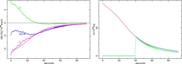
Figure 6. Left panel: the rate of decay of turbulent KE after oxygen burning and neutrino cooling are turned off. The dominant terms are shown:  is the increase of KE due to buoyant driving, dK/dt is the time derivative of the total KE in the convection zone, and
  is the inferred dissipation from the turbulent spectrum (dK/dt − B). We assume that little KE escapes the convection zone. The solid line shows the damping rate approximated by εK = −MCZ vrms3/ℓD with ℓD = 4.35 × 108cm. After 30 s, the buoyancy has died away but damping remains. Right panel: KE as a function of time (solid line), and fits of the damping after 40 s for ℓD/108 cm = 2.1, 2.6 (best), and 3.1. In this phase there is no driving to create anisotropy, and the flow becomes more isotropic on average.
Download figure:
Standard image High-resolution imageIf we neglect the small terms for energy flux escaping the convective zone, we may express the KE equation (Equation 1) more concisely as D = dK/dt − B, where D is the inferred dissipation. After 30 s, the buoyancy driving term B becomes small, and dK/dt tracks the turbulent dissipation D. Note that dK/dt is slightly below D, possibly because of entrainment of stable matter at the convective boundary which requires energy. If we globally fit the inferred damping term by εK = −MCZ v3rms/ℓD, we have ℓD = 4.16 × 108cm = 0.97 ℓCZ.
The right panel in Figure 6 shows a fit to the KE, starting 40 s after the burning was switched off, and the fossil buoyancy had died away. The KE may be represented analytically if dK/dt = D, so that this late part of the damping curve is reasonably well approximated by a lower damping length, ℓD = 2.6 × 108cm = 0.61 ℓCZ.
This independent simulation supports the identification of subgrid damping with isotropic Kolmogorov damping, and the representation of damping by the global expression (Equation 5), and ℓD ≈ (0.6 to 1.0)ℓCZ.
These and the previous estimates for ℓD seem to vary beyond the statistical accuracy of the analysis. Replacing the complexity of turbulent dissipation by the simple expression εK = −MCZ vrms3/ℓD, with constant ℓD is a vast change. This quantity ℓD is a property of the flow, and indirectly of the problem being addressed. In particular, the pure decay is more isotropic than the driven cases (Ogilvie 2003). As Table 3 indicates, the ratio ℓD/ℓCZ is different for different flows, but of order unity. Further investigation with different simulations and different physical parameters is needed to understand more precisely the general behavior of ℓD.
Table 3. Decay Lengths for Different Flows
| Flow | αD = ℓD/ℓCZ |
|---|---|
| Quasi-steady oxygen burning | 0.89 |
| Fossil buoyancy in decay | 0.97 |
| Pure decay | 0.61 |
Download table as: ASCIITypeset image
3. GENERAL EQUATIONS FOR STELLAR EVOLUTION
How is this approach related to the standard equations of stellar evolution?
3.1. Internal Energy Equation
In MLT a connection is made between superadiabatic gradient Δ∇ and convective velocity. This allows the convective enthalpy flux to be expressed in terms of Δ∇ (see, Kippenhahn & Weigert 1990, Section 7, Clayton 1983, Sections 3–5, and Hansen & Kawaler 1994, Section 5). The turbulent KE equation (Equation 1) can perform the same function, if the convective velocity is identified with the rms velocity  at a given radius, and used in the enthalpy flux in the same way. This replaces the parameterization used in MLT with a physical constraint.
We need to rewrite the total energy Equation (A6 in Meakin & Arnett 2007b) in the form of the internal energy equation used in stellar evolution. To get the internal energy equation, we subtract the KE Equation (A12) from the total energy Equation (A6), and find
The left-hand side is just ρ(dEI/dt + p0dV/dt) in Lagrangian (comoving) coordinates (Landau & Lifshitz 1959), defining ρ0 = 1/V, so that
The first line contains usual terms. Here Fr is the heat flux due to radiative diffusion, and in this frame the flux of internal energy FI becomes the enthalpy flux carried by convection Fe (see, Tennekes & Lumley 1972, p. 33, and our Equation 12). The nuclear heating term  includes neutrino cooling.
We will rewrite Equation (18) in a more familiar notation (see Arnett 1996, Clayton 1983, Hansen & Kawaler 1994, or Kippenhahn & Weigert 1990),
The first four terms contain the usual formulation. The new terms are:  which represents the compressional work done by pressure fluctuations (which also appears in the KE equation and we have seen it to be small here), εK/ρ0 which is the deposition of heat by the Kolmogorov turbulent cascade, and
  , which is zero in hydrostatic equilibrium without rotation or expansion, and drives meridional circulation for rotating, radiative stars (Tassoul 1978; Clayton 1983).
The εK/ρ0 term allows turbulent KE to do dissipative heating, a new effect not in conventional stellar evolution, and it is not guaranteed to be negligible. Through Equation (1) it couples the divergence of the KE flux (including rotational shear) and the wave energy flux to the internal energy. As an internal energy source term, it can generate entropy and cause mixing even in radiative regions. For the Sun, this term would give rise to heating in the photosphere, chromosphere, and corona by shocks and wave motion (pressure and Alfven waves), for example.
Equations (1) and (19) represent an extension of turbulent convection theory for stellar evolution, in which (1) the algebraic relation for convective velocity and superadiabatic gradient is replaced by a differential equation (see Spiegel 1972), and (2) the Kolmogorov cascade is explicit in the formulation. Note that both space and time derivatives appear, making the system nonlocal and time dependent, unlike MLT. These derivatives allow the treatment of boundary dynamics in a physical way. We will explore specific implementations in a subsequent paper, including entrainment at convective boundaries.
Let us now consider some simplifications in order to clarify the meaning of these equations. In particular, we assume time invariance (so the time derivatives are small on average), no overall background motion (u0 = 0), and little work done by pressure perturbations on the velocity perturbations. As shown previously, these are reasonable approximations except in extreme cases. Then Equation (1) becomes

and Equation (19) becomes

The coupling of internal energy and turbulent KE occurs through the Kolmogorov cascade, which creates internal energy by damping KE. Eliminating εK, we have

In a steady state, the nuclear energy generation must balance the divergence of fluxes out of the region and supply the work needed to maintain the convective flow. This is different from the usual formulation used in stellar evolution in that there are new terms  ), which combine to equal εK, the dissipation rate due to the Kolmogorov turbulent cascade. If the turbulent velocity is nonzero, these corrections are also nonzero, leading to the conclusion that the standard formulation of stellar evolution is wrong in neglecting turbulent heating. The motion implied by convection will carry KE, drive pressure and gravity waves into radiative regions, and give local microscopic heating as it dissipates in a transit time, effects that should no longer be ignored in stellar evolution. Through its dependence on ζ, for a given convective enthalpy flux, the KE flux is dependent upon the equation of state.
For a low Mach-number flow,

and radial coordinates so that ∇ · F → dL/dm, then Equation (22) becomes
where ∇ = βTPV/CPT, mp = 4πr2ρHP, and HP is the pressure scale height. For an ideal gas, ∇ → (γ − 1)/γ, or 0.4 for γ = 5/3. For gases with a specific heat at constant pressure which is large compared to the specific heat at constant volume (such as partially ionized plasma or electron–positron plasma), ζ is considerably smaller (see below).
4. COMPARISON TO OTHER SIMULATIONS
These theoretical ideas may be tested by application to other simulations of turbulence. Several groups have compared 3D simulations to MLT predictions (Chan & Sofia 1989, 1996; Kim et al. 1995, 1996; Meakin & Arnett 2007b; Porter & Woodward 2000; Porter et al. 2000), and published sufficient detail to allow easy quantitative comparison. All agree that MLT is somewhat successful, but derive different values for some of the MLT parameters. This suggests that these parameters may not be universal, but a function of the conditions of the simulated flow, and that our theoretical analysis may be able to put them on a common basis. See also Abbett et al. (1997), Ludwig et al. (1999), Trampedach et al. (1999), and Brandenburg et al. (2005), who have also compared simulations with MLT.
These simulations are not a homogeneous set, so that global comparisons on this data set must be taken with caution. Porter & Woodward (2000) and Meakin & Arnett (2007b) used PPM codes while the Yale group (Chan & Sofia 1989, 1996; Kim et al. 1995; Robinson et al. 2004) used compressible viscous codes with subgrid scale modeling (and much lower resolution). Chan & Sofia (1996) and Meakin & Arnett (2007b) had the convection zone bounded by stable regions while the others did not; these boundary conditions give rise to new phenomena (Meakin & Arnett 2006, 2007a). The deeper convection zones developed more anisotropic flows, and velocities approaching the sound speed (e.g., Cattaneo et al. 1991; Woodward et al. 2003). Porter & Woodward (2000) carefully attempted to compensate for these effects, the Yale group used damping to tame them, and the soft equation of state and shallower depth made them small for Meakin & Arnett 2007b, see below). Porter & Woodward (2000) found that they needed to shift the apparent mixing length by about 30%, down from α = 3.53 to α = 2.68. The simulations of Meakin & Arnett (2007a) included an oxygen-burning shell (with an electron–positron equation of state, see Table 5), and those of Kim et al. (1995) and Robinson et al. (2004) included a solar photosphere (with strong ionization effects in the equation of state). Our simulations are driven by nuclear heating at the bottom of the convection zone; the others are driven by cooling at the upper boundary (like the Sun).
Table 4 summarizes the inferred parameters. The entries are ordered in increasing depth of the convective zone as measured in pressure scale height units (ℓCZ/HP), which corresponds to increasing asymmetry in the vertical direction. The choice of equation of state (ideal gas, e−e+-pair gas, ionized plasma) and of the boundary conditions affect the simulations. Even the definition of the depth of the convective zone may be modified depending on whether the grid includes the stable bounding region ("yes") or not ("grid"). The bottom line in the table gives the traditional MLT values for several parameters (Kippenhahn & Weigert 1990). The last column gives the number of zones on the computational grid.
Table 4. A Comparison of Parameters from Some 3D Simulations
| Reference | ℓCZ/HP | αT | αE | αv | EOS | Bnd. | Zones |
|---|---|---|---|---|---|---|---|
| Meakin & Arnett (2007b) | 2.0 | 0.73 | 0.70 | 1.22 | e-Pair | Yes | 4.0(6) |
| Porter & Woodward (2000) | 4.5 | 2.04 | 0.80 | 2.70 | Ideal | Grid | 6.7(7) |
| Chan & Sofia (1989) | 4.8 | 1.05 | 0.83 | 2.16 | Ideal | Grid | 3.6(4) |
| Kim et al. (1995) | 6.0 | 1.42 | 0.85 | 2.16 | Ionize | Yes | 3.3(4) |
| Chan & Sofia (1996) | 6.8 | 1.30 | 0.68 | 2.60 | Ideal | Yes | 4.8(5) |
| MLT | α/2 | 1.0 |  |
Download table as: ASCIITypeset image
4.1. Convection Parameters
We now examine each of a set of important convection parameters (see Porter & Woodward 2000 and Meakin & Arnett 2007b for details). These parameters reflect the various uses of the MLT parameter α, and are a convenient and concise way to compare the simulations of compressible turbulent convection.
4.1.1. αT
In 3D simulations, a correlation is found between rms temperature fluctuation  and the superadiabatic gradient Δ∇ = ∇ − ∇a − ∇x, using the conventional notation in astrophysics of ∇ = ∂ln T/∂ln P (Kippenhahn & Weigert 1990; Hansen & Kawaler 1994; Clayton 1983). Here, ∇a = ∂ln T/∂ln P, taken at constant entropy and composition, and ∇x = −∇μ is the remaining part due to possible compositional change. Then,

on average, over time and over the volume of the convection zone. Consider low Mach-number flow so that ρ'/ρ0 = −βT(T'/T0).
In a single convective roll (e.g., Lorenz 1963; Tritton 1988), T' is the temperature perturbation amplitude at the horizontal midplane. In the vertical midplane of the roll, T' = [(dT/dr) − (dT/dr)ad]ℓCZ/2 is the corresponding amplitude. Assuming the amplitudes are comparable,

implying that αT ≈ ℓCZ/2HP, and not a constant. In MLT, αT = α/2, which is a particular choice for the assumed flow.
In the simple picture of a single convective roll, (T')rms/T0 can give a buoyancy torque, while Δ∇ cannot, because the gravitational acceleration vector is directed radially downward (Tritton 1988). In the Lorenz (1963) model of thermal convection, the difference between the two is intimately connected to the onset of chaotic behavior. Meakin & Arnett (2007b) find αT ≈ 0.73 (see their Figure 17), so that

There is considerable variation in the values of αT shown in Table 4, with a tendency to increase for deeper (more stratified) convection zones.
Note that for two convective rolls, one atop the other, we would expect the characteristic roll size to change (ℓ ≈ ℓCZ → ℓCZ/2, so αT → αT/2, approximately). This explicitly shows how the convection parameters can be a function of the properties of the flow itself.
Figure 7, left panel, shows the behavior of αT as a function of the depth of the convection zone, for the computations listed in Table 4. The two PPM calculations (Meakin & Arnett 2007b; Porter & Woodward 2000) agree with the scaling indicated in Equation (27). The calculations using the compressible viscous equations with subgrid modeling for dissipation all lie below Equation (27). In order to give some idea of the depth needed in simulations of stellar convection zones, the x-axis in Figure 7 is marked from zero to the depth of the solar convection zone (20 pressure scale heights). None of these simulations describe such an extremely anisotropic case.

Figure 7. Predicted 2αT = αΛ,T (left panel) and  (right panel), as a function of depth of the convective zone in units of HP. This scaling (Meakin & Arnett 2007b) gives "alphas" which are comparable to the MLT values and each other. Some of the error bars are large; new simulations are needed to determine how well such results follow a single curve (C. Meakin & D. Arnett 2008, in preparation). In the limit of small depth, the mixing length must be no larger than the depth itself; hence the point at zero depth is an analytic result. The Meakin & Arnett (2007b) and Porter & Woodward (2000) points and the origin are close to colinear. It appears that both αT and αv are functions of depth of the convective region, and not universal constants.
Download figure:
Standard image High-resolution image
4.1.2. αE and αK
The enthalpy flux is
where Meakin & Arnett (2007b) find αE = 0.70 ± 0.03; in Table 4, αE is relatively constant among the simulations (the total range is about 20%). It is not ruled out that αE might be a universal constant, or at least slowly varying. Note that αE is just the correlation coefficient for T' and u'. It seems that αE is not sensitive to the Prandtl number Pr. Porter & Woodward (2000) have a different Pr (ours is Pr ≈ 1) and get an αE similar to ours.
Using Equation (25), this becomes

Similarly, if the KE flux is
we may define

so that  . Note that the sign of αK can be negative.
4.1.3. αv
In Meakin & Arnett (2007b), the correlation between convective velocity (squared) and superadiabatic excess Δ∇ is written as

In MLT, a similar expression is defined, with α2/8 replacing α2v/4. If we have local balance between buoyancy driving and turbulent damping,

Using Equations (13), (25), and (28), we have

Comparing this to Equation (32) we have

Using Equation (27) and αE = 0.70,

In Table 4, we see that αv is variable, and tends to increase with increasing depth of the convective zone. This is shown explicitly in the right panel of Figure 7. The two PPM calculations are in excellent agreement with Equation (36), taking ℓD = 0.9 ℓCZ (αD = 0.9), while the three compressible viscous calculations lie below it.
Using Equation (29), we have

Using Equation (27), Equation (36), ℓD = 0.9ℓCZ, and αE = 0.70, we have

for the factor in Equation (37).
4.2. The Electron–Positron Plasma
The thermodynamic character of the electron–positron plasma in the oxygen-burning shell is significantly different from an ideal gas, an effect which must be taken into account in comparisons to simulations which use different equations of state. This is illustrated in Table 5; we use the Helmholtz equation of state of Timmes & Swesty (2000). The entropy in the oxygen burning convection zone is  in dimensionless units, where
  is the gas constant. The zone is about 2 pressure scale heights deep (see Column 3). For an ideal gas, the specific heat at constant pressure is
  ;
;  is much larger for the plasma, ranging between 10 and 16 (Column 4). Column 5 gives the value of βT, which is unity for an ideal gas, but lies between 3 and 4 for the plasma. Column 6 gives the ratio of PV/CPT = p0/ρ0CPT0, which is 0.4 for an ideal gas. The ratio of the buoyancy flux to the enthalpy flux (Equation (14)) is proportional to ∇ = βTPV/CPT. The same factor appears in the ratio of the KE flux to the enthalpy flux. For the ideal gas ζ = 0.4, but is smaller for the plasma (Column 7). For the same convective enthalpy flux, the pair-plasma has a much lower KE flux, so the velocity scale is lower.
Table 5. Thermodynamic Parameters for Entropy 
| T9 | ρ6 | ln Pmax/P |  |
βT | PV/CPT | ∇ad |
|---|---|---|---|---|---|---|
| 2.51 | 1.580 | 0.0 | 15.36 | 3.912 | 0.0609 | 0.2382 |
| 2.31 | 1.225 | 0.348 | 14.53 | 3.757 | 0.0638 | 0.2397 |
| 2.11 | 0.930 | 0.724 | 13.62 | 3.592 | 0.0673 | 0.2417 |
| 1.91 | 0.690 | 1.134 | 12.67 | 3.421 | 0.0714 | 0.2443 |
| 1.71 | 0.498 | 1.583 | 11.73 | 3.257 | 0.0762 | 0.2483 |
| 1.51 | 0.348 | 2.080 | 10.83 | 3.106 | 0.0814 | 0.2529 |
Download table as: ASCIITypeset image
4.3. Direction of the KE Flux
The KE flux is averaged over angle at a given radius, and averaged over two convective turnover times. As Figure 5 shows, this time span covers significant dynamic behavior. Roughly speaking, an unstable configuration forms, becomes dynamic, reforms, becomes dynamic again, and so on. Over this turnover timescale the nuclear burning provides the energy necessary to drive the turbulent KE  .
.
The convective instability is closely related to the Rayleigh–Taylor instability (Chandrasekhar 1961a), which has been produced dramatically in high energy–density plasma experiments (Remington et al. 1999), i.e., under star-like conditions and well into the nonlinear growth regime. The characteristic behavior is the rise of mushroom-shaped higher entropy plasma and the fall of spike-shaped lower entropy plasma. If we consider a closed volume, these motions are accompanied by slower return motions which maintain mass conservation. The KE flux scales with velocity cubed, and so is dominated by the fast moving mushrooms and spikes. In a symmetrical system, we will have an upward KE flux (from the mushrooms) in the region above the horizontal midplane of the volume, and a downward KE flux in the region below. If we average over several cycles (turnover times) the KE flux will be dominated by these motions, being positive (upward) above the midplane and negative below. This is qualitatively similar to the simulation results of Meakin & Arnett (2007b; see their Figures 21 and 22).
This simple picture is complicated by an up–down asymmetry due to stratification (hydrostatic structure). The depth of the convection zone in pressure scale heights, ℓCZ/HP = ln(Pbot/Ptop), is a direct measure of the up–down asymmetry. Upward flows move into regions of lower pressure, and expand; downward flows move into regions of higher pressure, and are compressed. The smaller area of the downflows implies higher velocities relative to a coordinate frame containing the convection zone (a Lagrangian frame). This will favor downward (negative) KE fluxes. The neglect of KE fluxes (Böhm-Vitense 1992) corresponds to the limiting case of a shallow convection zone. For deep convection zones, there is a strong bias in favor of fast downward plumes (Nordlund & Stein 2000; Stein & Nordlund 1998), and these dominate the flow for simulations with ℓCZ/HP ⩾ 4 or so. In Meakin & Arnett (2007b), which has a depth ℓCZ/HP = 2, the convective zone is skewed, so that the surface, which separates the positive and the negative KE fluxes, moves nearer to the bottom of the convection zone. For Porter & Woodward (2000), where ℓCZ/HP is larger, the positive KE flux is overwhelmed, and the direction of the KE flux is opposite to that of the much larger enthalpy flux. We expect this to be a general property of deep convection zones.
There is a natural limit to the depth of convection zones expected in active burning regions. Entropies in active burning regions vary relatively slowly (Arnett 1996), so that the depth of a convection zone implies a value of the temperature ratio between bottom and top. In Table 5, the convection zone extends down almost to neon burning temperatures (T ≈ 1.5 × 10⁹K). Further extension will entrain new fuel into the oxygen convective shell, which will burn at the top of the convection zone, choking the flow. For the last stages (C, Ne, O, and Si burning), the burning temperatures for different fuels are fairly close together, implying that their related convection zones will tend to be relatively shallow. They are also close together in radius, raising the issue of interactions between them (Meakin & Arnett 2006).
Here  . For example, for advanced burning stages or radiation dominated regions, γ ≈ 4/3, and γ/(γ − 1) = 4. For helium and hydrogen burning, T(He)/T(H) ≈ 13 so ℓCZ/HP ⩽ 4ln 13 ≈ 10. A helium burning convective zone will not be deeper than about 10 scale heights unless the overlying matter is devoid of hydrogen. For carbon burning the corresponding depth is ℓCZ/HP ≲ 3, unless devoid of H and He fuel. Surface convection zones may extend down to the hydrogen burning regions. Very roughly, ln T(H)/Te ≈ 8, so ℓCZ/HP ≲ 32, using the structure of an n = 3 polytrope.
4.4. Magnitude of the Kinetic Energy Flux
Table 6 gives the ratio of kinetic energy flux to enthalpy flux for several 3D simulations. This ratio is much smaller in our simulations (by a factor of ∼20–40) than in the others, and FK changes sign in our convection zone.
Table 6. Comparison of Some 3D Simulations
| Reference | lCZ/HP | ∇a | FK/Fc |
|---|---|---|---|
| Meakin & Arnett (2007a) | 2 | 0.24 | −0.018 |
| +0.014 | |||
| Porter & Woodward (2000) | 4.5 | 0.40 | −0.3 |
| Cattaneo et al. (1991) | 5 | 0.40 | −0.35 |
| Chan & Sofia (1989) | 4.8 | 0.40 | −0.35 |
| Chan & Sofia (1996) | 6.8 | 0.40 | −0.50 |
Download table as: ASCIITypeset image
As in Meakin & Arnett (2007b), we can write the KE to enthalpy flux ratio according to mixing length relationships,
and then balance between buoyancy driving and turbulent damping through Equation (37) gives
See Equation (3.14) of Porter & Woodward (2000), which uses a gamma-law equation of state to generate the sum of kinetic and enthalpy fluxes, and implies an equivalent flux ratio.
The ratio of ∇ad for the ideal gas to that of the electron–positron gas gives a factor of 1.6 or so. The ratios of the depth of the convection zones give another factor of ∼5. While these considerations illustrate the role played by the depth of the convection zone and go some way towards explaining the trends in KE flux it is also important to consider the geometry of the driving region, which relates to how well a local balance between buoyancy driving and turbulent damping is achieved as assumed in Equation (37). In particular, the length scale la over which buoyancy is imparted to the stellar plasma through either heating at the base of the convection zone or cooling at the top can affect the KE to enthalpy flux ratio dramatically. This may be understood simply: the flow depends both upon the geometry of the convective domain and upon the way in which the fluid is stirred. At present we have at least two basic patterns, a mostly negative kinetic energy flux for deep convective zones driven by surface cooling (most stellar surface convection zones) and a more complex positive-negative convective flux for shallower zones driven by nuclear burning. More simulations are underway to clarify this issue (C. Meakin & D. Arnett 2009, in preparation).
4.5. Saturation of Kinetic Energy Flux
Are there limits to the linear rise in energy of convection that is implied by Figure 7? Deep convection zones (ℓCZ ⩾ 3HP) have strong negative KE fluxes. For very deep zones, the extrapolated kinetic fluxes imply supersonic velocities. Such large velocities would generate shock waves, which would increase dissipation, converting KE into internal energy. The rate scales as the velocity difference cubed, which is the same scaling as turbulent dissipation in the Kolmogorov cascade (Bethe 1942; Boris 2007). This suggests that even if deeper convection zones did tend to have increasingly strong velocities, shock dissipation will become significant, and resist the increase of ℓD with increasing ℓCZ. In this sense, the increase in damping length must "saturate" with increasing depths.
Increased damping may come sooner from another effect: a change in the nature of the eddies and the size of the damping length. Physically this would occur as follows: as the deep, fast, narrow downflows drive into the convection zone they will give rise to shear instabilities at their interfaces, which will lead to mixing with the ambient fluid, and exchange momentum through a turbulent viscosity, and eventually completely dissolve into the background. This would give shorter dissipation lengths, and would begin to occur before the Mach numbers become large enough for significant shock formation.
We expect the PPM calculations for deeper convective zones to "flatten" in Figure 7 as the Yale simulations do, but at higher amplitude, as a result of higher damping rates. This hypothesis needs to be tested numerically, which will be challenging. Shock waves may cause errors at grid boundaries, deep convection zones will have longer thermal relaxation times, and maintaining sufficiently wide aspect angle implies many computational zones for adequate resolution, for example.
The simulations of the Yale group (Chan & Sofia 1989, 1996; Kim et al. 1995, 1996; Robinson et al. 2004), which use fewer zones and a strong damping (Smagorinsky 1963), appear to have a larger dissipation than the PPM simulations (Porter & Woodward 2000; Meakin & Arnett 2007b). This is qualitatively equivalent to the saturation discussed above, and may be tested if calculations using the Yale code (or equivalent) are repeated at higher resolution and/or lower dissipation.
5. SOME IMPLICATIONS
5.1. Waves
The energy flux terms include both advective transport and waves. Here we will recall some properties of waves and their generation (Landau & Lifshitz 1959; Press 1981). The characteristic frequencies of convective motion are centered about a frequency ωCZ ≈ vrms/ℓCZ. The convective Mach number,  , is a measure of compressibility of the flow; here
  is the sound speed. If the interface between convective and radiative zones moves with the matter (is volume conserving, on average), it generates acoustic waves by dipole emission at a luminosity Lp-mode ∝ ω6CZ (see, Landau & Lifshitz 1959, Section 73), or as the Mach number to the sixth power. For more vigorous motion, the perturbation may give volume changes, so that the acoustic wave generation by monopole emissivity, or Mach number to the fourth power. For subsonic flows this channel is closed to significant energy flow, but open as (u')rms approaches the local sound speed, as it does in the surface convection zones of many stars, including the Sun, or as it may in the stage prior to core collapse in massive stars.
While the exact power dependence may depend upon specific geometries and degree of interference, a general result seems to be: the gravity wave channel dominates over the acoustic channel for low Mach-number flows (as we observe in our simulations; see Meakin & Arnett 2007a for a more detailed discussion of both the g-mode and p-mode behaviors, including mixed p- and g-modes). Both types of waves are generated by convection interacting with stably stratified bounding regions, and the luminosity of each depends upon both the convective vigor and the impedance at the boundary. Such waves can propagate into stably stratified regions (Press 1981; Press & Rybicki 1981; Young & Arnett 2005). Generation of gravity waves by convective turbulence has become an issue in questions of mixing and angular momentum transport (García López & Spruit 1991; Charbonnel & Talon 1999; Talon & Charbonnel 2004; Young & Arnett 2005).
The establishment of a robust estimate of the turbulent velocity field should improve estimates of wave generation, which has implications for mass loss, mixing in radiative regions, coronal heating, and helioseismology. In particular, the pressure correlation flux takes over the energy carried by the KE flux as the convective boundaries are approached. This gives a direct connection between the scale of turbulent velocity and g-mode wave emission (Press 1981).
5.2. Rotation and Magnetic Fields
A closely similar set of mean-field equations is used in the theory of the magnetic resonance instability (MRI) in accretion disks (Balbus & Hawley 1998; Pessah et al. 2006). If we had included magnetic fields in the MHD approximation, and assumed strong rotation, our procedure would have produced an equation for mechanical energy(our Equation (1) corresponds to Equation (17) of Balbus & Hawley 1998), and total energy (Equation (A6) of Meakin & Arnett 2007b to their Equation (27)). Projection onto a cylindrical coordinate system, with the rotational axis oriented parallel to the total angular momentum vector, would give an angular momentum equation (their Equation (29)). Auxiliary equations provide for magnetic field dynamics, radiation transport, and nuclear burning. This underlying similarity provides a way to write a more general set of mean-field equations, of which both stars and accretion disks are limiting cases. In turn this allows a systematic evaluation of the relative importance of different effects (rotational mixing and convective mixing, for example) which are now considered piecemeal.
Our simulations include the complete set of rotational terms, but the initial conditions imply that these terms are not exercised except as convectively induced shear. Our simulations do not include magnetic fields in the MHD approximation, but could be generalized to do so (Stone & Gardiner 2007; Pessah et al. 2006). Because they interact, rotation and magnetic fields should be included together.
Balbus & Hawley (1994) have argued that in the stellar case, the weak-field MRI dominates over merely hydrodynamic instabilities, and drives the radiative zones (but not convective zones) toward solid body rotation. Heger et al. (2000) argued the reverse (based on the Høiland instability criterion), that convective zones would tend toward rigid body rotation, and radiative zones would tend to have differential rotation. Because the Høiland instability applies to neutral fluids, not dense plasma, it is probably not relevant for stars. Helioseismology (Thompson et al. 1996; Howe et al. 2005; Brandenburg 2007) is showing that while the convective zone of the Sun shows differential rotation, the underlying radiative zone seems to be tending toward solid body rotation, as the MRI arguments suggest. Browning & Basi (2007) have shown that even deep convection zones can generate significant magnetic fields, so that the presence of a stable interface is not necessary for field generation. The rotational state of the central regions of the Sun probably depends upon the efficacy of angular momentum transport by processes related to flow of the plasma, including g-mode waves (Charbonnel & Talon 1999), as well as magnetic fields.
5.3. Damköhler Number for Burning
In general, it is appropriate to decompose the equations in temperature (T = T0 + T') and composition as well. The opacity and the nuclear reaction rates are often sensitive to both. Meakin & Arnett (2006) found flashing due to oxygen burning in vigorous downdrafts which were fuel-rich (the flashes were too mild to affect the flow dramatically). None of these effects are included in standard stellar evolution theory. For simplicity we suppress this complication for the moment; this means that our opacities and reaction rates are to be interpreted as averages over fluctuations in these variables as well. Further investigation of this issue, with 3D simulations, is desirable.
For this set of simulations, the heating and cooling times are at least 100 times longer than the transit times, so that we are in the regime of small Damköhler number Dm ≲ 0.01 (Zel'dovich et al. 1985; Oran & Boris 1987). The release of nuclear energy during a transit time is small relative to the internal energy in the convection zone, but comparable to the superadiabatic energy and to the turbulent KE. The burning drives the turbulent motions, but only gives moderate pulses of KE, as shown in Figure 5. This is unlike the much more complex problem of Type Ia supernova models, for which Dm is large. In our case the necessary averaging over convective cycles does not seem to be a problem.
This convenient state may not apply to the double shell flash stage for asymptotic giant branch (AGB) stars, in which wave-driven mixing and entrainment are likely to complicate the issue of mixing, and therefore figure into the question of s-process nucleosynthesis (Busso et al. 1999; Campbell & Lattanzio 2008).
6. SUMMARY
We find that our 3D time-dependent simulations of compressible stellar turbulence (ILES) are well represented by a master equation (Equation (1)) for KE which includes dissipation implied by the Kolmogorov cascade. The damping length is found in three independent ways, with reasonable consistency, and is the size of the largest eddy, which is approximately the geometric linear dimension (depth) of the convective zone. Unlike the mixing length of MLT, it is not a free parameter, but a mathematical consequence of the turbulent flow. Balancing turbulent buoyant driving with Kolmogorov damping provides a reasonable estimate of the damping length. The divergence of KE and acoustic fluxes is nonzero, and provides the mechanism to spread turbulence through the convective zone, and make the Kolmogorov damping a good approximation. The turbulent flow is highly dissipative and must be maintained by continual driving; this "frictional heating" term is missing from the standard stellar evolution equations, as are the KE and acoustic fluxes.
Fluctuations in KE are significant (of order 50%), and damping lags driving by about a transit time for the convective zone.
Comparisons with some other simulations, which were dramatically different in many respects, gives a consistent picture. Turbulent convection is more vigorous for deeper (more stratified) convection zones. Turbulent KEs are lower for nonideal equations of state, such as partially ionized plasmas and electron–positron plasmas, to the extent that their specific heat at constant volume is less that their specific heat at constant pressure. The average flow structure changes in a simple way depending upon the depth of the convection zone; deep convection zones have downwardly directed flows of KE, canceling some of the upward enthalpy flux.
It appears that extension of this approach, using simulations to define stellar convection algorithms, can establish a theoretical model of turbulent convection that does not require astronomical calibration, but can be based upon a combination of computer simulations, terrestrial observations, and experiments. Efforts to implement this general theory in a stellar evolution code are underway.
During the course of this project, we lost two friends who were leaders in the field of stellar evolution, John Bahcall and Bohdan Paczynski, to whom this paper is dedicated. This work was supported in part by NSF Grant 0708871 and NASA Grant NNX08AH19G at the University of Arizona, and the ASCII FLASH center at the University of Chicago, D.A. thanks the Aspen Center for Physics and the International Center for Relativistic Astrophysics (ICRA) for their hospitality, Brian Chaboyer for help with the history of the mixing length implementation, Martin Pessah for discussions of MRI physics, Robert Stein for discussion of the effect of the continuity equation on flows, Vittorio Canuto for helpful discussions of the philosophy of turbulence modeling, Martin Asplund for providing machine-readable copies of solar surface models, and Frank Timmes for helpful comments on the draft and for providing access to the Saguaro computer cluster. We thank an anonymous referee for insightful comments which improved both our presentation and our understanding.
APPENDIX: DECOMPOSITION
We decompose velocity, density, and pressure fields into mean and fluctuating components according to

where  and
and  and the overbar and brackets indicate time and horizontal averaging, respectively. For data handling and analysis purposes we consider the fluctuating component of the field to be composed of a radial p-mode component and a component due to all other sources
This additional decomposition allows us to make a more accurate estimate of the fluctuations associated with turbulent convection in the presence of a coherent radial p-mode which is not well sampled in the output files from the simulation. If the radial p-mode contribution were well sampled then we would find  to the degree that the mode is adiabatic.
Consider the radial velocity to be composed of the following components
where u0 is the mean background expansion, u'p is the radial p-mode-induced fluctuation, and u't is the fluctuation due to turbulent convection and other nonradial modal components. Averaging, we find
Because of our poor sampling of the low-order radial p-modes which have frequencies comparable to the simulation data output rate (δt ≈ 0.5 s) we find that the term  and contributes a significant error to the estimation of u't. In order to correct for this horizontally coherent p-mode-induced radial displacement, we subtract the horizontally averaged radial velocity component at each time step and estimate the turbulence-induced fluctuation by

The latter approximate equality in the above equation is made because of the smallness of the background expansion compared to the rms velocity fluctuations associated with the turbulent convection, u0/u'c ∼ 10−3.
The instantaneous fluctuations in pressure and density are calculated according to

and,

Footnotes
- 5
The shear from convection is similar to the shear from differential rotation; fluid experiments may use either to investigate the physics of shear (Turner 1973). Although different in some details, there are deep connections between convective mixing as described here and the rotational mixing investigated by Meynet & Maeder (2000).
- 6
Porter & Woodward (2000) suggest that large-scale flows do dominate the energy flux.
- 7
As we discuss below, simulations with stiffer equations of state will have larger pressure fluctuations. We expect the neglected terms to be important for wave generation, but probably in a restricted volume of the convection zone.
- 8
In Meakin & Arnett (2007b) we denoted this quantity by βT; the subscript T is to avoid confusion both with Eddington's use of β for the ratio of gas to total pressure, and the fluid dynamics community use of β as the adverse temperature gradient.
- 9
In implicit large eddy simulations (ILES) like this, the numerical cascade only goes down to the grid scale.