


ABSTRACT
Analysis of the proper motions of the subparsec scale jet of the quasar 3C 279 at 15 GHz with the Very Long Baseline Array shows significant accelerations in four of nine superluminal features. Analysis of these motions is combined with the analysis of flux density light curves to constrain values of Lorentz factor and viewing angle (and their derivatives) for each component. The data for each of these components are consistent with significant changes to the Lorentz factor, viewing angle, and azimuthal angle, suggesting jet bending with changes in speed. We see that for these observed components Lorentz factors are in the range Γ = 10–41, viewing angles are in the range ϑ = 0 1–50, and intrinsic (source frame) flux density is in the range, Fν, int = 1.5 × 10⁻⁹–1.5 × 10⁻⁵ Jy. Considering individual components, the Lorentz factors vary from Γ = 11–16 for C1, Γ = 31–41 for C5, Γ = 29–41 for C6, and Γ = 9–12 for C8, indicating that there is no single underlying flow speed to the jet and likely we are seeing pattern speeds from shocks in the jet. The viewing angles vary in time from 06 to 15 in the case of C1 (the least extreme example), from 05 to 50 in the case of C8, and from 01 to 09 for C5 (the last two being the most extreme examples). The intrinsic flux density varies by factors from 1.4 for C8 and 430 for C5. Theoretical analysis of the accelerations also indicates potential jet bending. In addition, for one component, C5, polarization measurements also set limits to the trajectory of the jet.
Export citation and abstract BibTeX RIS
1. INTRODUCTION
Historically, there has been great interest in the study of quasar 3C 279. It is one of the brightest extragalactic radio sources and the first to have observed superluminal motion (Cohen et al. 1971; Whitney et al. 1971). In addition, 3C 279 undergoes dramatic optical flares on a regular basis, and was the first gamma-ray blazar discovered by the EGRET instrument on board the Compton Gamma Ray Observatory (Hartman et al. 1999). More recently, 3C 279 has also been continuously detected by the Large Area Telescope (LAT) instrument on the Fermi Observatory (Abdo et al. 2010). All these phenomena are thought to be related to the quasar's relativistic jet and its emission properties. Increasingly, the very long baseline interferometry (VLBI) technique, particularly since the advent of the Very Long Baseline Array (VLBA) in 1994, has been able to probe these jets on milliarcsecond scales at high resolution. One of the main goals has been to tightly constrain the kinematic properties of the jets, such as viewing angle (ϑ), speed (β = v/c), Lorentz factor (Γ), and relativistic Doppler beaming factor (δ).
Detailed analysis of 3C 279's milliarcsecond scale radio jet has been conducted by Homan et al. (2003) at 15 GHz who note a bent path for the outermost feature labeled as C4 (currently labeled as C1 in Lister et al. 2009b), leading from parsec to kiloparsec scales. Wehrle et al. (2001), using data at 22 GHz and 43 GHz, reported a curved trajectory for C4 during 1991–1997. They use these data to constrain the viewing angle to 2°. Jorstad et al. (2004) confirm the C4 bending from 43 GHz monitoring observations. Our present work uses the MOJAVE data set for quasar 3C 279 from epoch 1995.57 to 2010.82 (Lister et al. 2009a). For the remainder of this paper we use the component naming conventions of Lister et al. (2009b). To aid in visualizing these components, we include a labeled 15 GHz map from 2003 (Figure 1). In the remaining sections, we use the analysis techniques of Homan et al. (2001, 2003) to determine the trajectory of each of the superluminal components previously determined to exhibit significant accelerations (Lister et al. 2009b). We have adopted the cosmology Ωm = 0.3, ΩΛ = 0.7, and H0 = 70 km s−1 Mpc−1. In Section 2, we discuss the nature of our data set; in Section 3, we present the analysis of these data, focusing on the constraints on kinematics provided by the accelerations, flux densities, and additional data; in Section 4, we discuss the broader physical relevance of this analysis; and in Section 5, we present our conclusions.
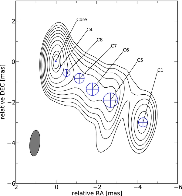
Figure 1. 15 GHz VLBA contour map of 3C 279 at epoch 2003.46 (June 15). This image is fitted with circular Gaussian components modeling the bright features. The map peak flux density was 8.3 Jy beam−1, where the convolving beam was 1.3 × 0.5 mas at position angle (P. A.) of −60. The contour levels were drawn at 0.2%, 0.5%, 1%, 2%, 4%, 8%, 16%, 32%, 64%, and 80% of the peak flux density. The bright components are labeled. The Gaussian components are overlaid on the map.
Download figure:
Standard image High-resolution image2. DATA
3C 279 has been regularly observed with the VLBA at 15 GHz as part of the MOJAVE Survey (Lister et al. 2009a), and prior to that, as part of the 2 cm Survey (Kellermann et al. 1998) since 1993. Details of the observing program can be found in Lister et al. (2009a). In addition, these data were supplemented with many epochs of data available in the VLBA archives from this period. The data were first edited and calibrated using AIPS (Bridle & Greisen 1994). Caltech's DIFMAP package was then used for self-calibration, mapping, and modeling (Shepherd 1997). The detailed modeling results are presented in Lister et al. (2009b). Here, as in the aforementioned work, we have assumed components to be circular Gaussians. As stated in Lister et al. (2009b), there is about a 5% uncertainty in the flux densities. The positional uncertainties will be approximately 0.2 mas. Thus, in most cases, our components' positional uncertainty will be less than or close to 10%. As previously mentioned, we have limited ourselves to studying the components that have exhibited significant accelerations (Lister et al. 2009b); however, we have recalculated the accelerations of these components based on the most recent data (see Table 3).
3. ANALYSIS
3.1. Using Proper Motion and Flux Density to Constrain Kinematic Parameters
We begin the analysis by calculating the values of the apparent speed, βapp (see Equation (1)), from the proper motion, μ. The proper motion, μ, is the slope of the linear regression to the component distance from the core versus time, as seen in Figures 2–5. We can clearly see that some of these fits will be closer to linear (such as C8) whereas a component such as C5 shows very complex changes and C6 shows movement from core that clearly implies rapidly increasing apparent speed. As a first approximation, we use just the linear fit for now and apply the standard formulae:

where dθ is the angular size distance in Mpc and z is the cosmic redshift. A derivation of Equation (1) can be found in Pearson & Zensus (1987) and Porcas (1987).
We then use βapp (see Equations (2) and (3)) to constrain the Lorentz factor, Γ, and the viewing angle, ϑ. Here, the viewing angle refers to the angle between the direction of motion of the relevant component and the line of sight to the observer, as measured from the observer's frame:
where β refers to the speed, v, divided by the speed of light, c.
Then, using Equations (4) and (5), we can best determine which range of values of the intrinsic flux density, Fν, int, and the relativistic Doppler beaming factor, δ, best fit the observed flux densities (Figures 6–9), Fν, obs, at a given time:

Here, α refers to the spectral index assuming Fν∝ν−α. We have assumed α = 0.8, which is commonly the case, at least approximately, for blazar components that have long ago merged with the core. We note that the kinematics are not at all dependent on this assumption, and the results concerning level and variability of flux density are dependent on this in a predictable way (by inverting Equation (5)). Furthermore, we can see that the general results concerning variability and how that ties in to the kinematics are not highly dependent on spectral index. Here, if we take the ratio of two flux densities from two different times (labeled with subscripts 1 and 2), then
If we assume that δ2/δ1 is no larger than about 1.65 (the maximum in our set of observations of all of these components), and we assume liberally that α can be in the range of −1 to 1, then, after substituting into Equation (6), the range of intrinsic flux ratios that we calculate can differ by a factor of about 2.7. Therefore, for a typical case, it is unlikely that our results will be critically dependent on assumptions regarding spectral index.
We note that all components show a decreasing observed flux density, which is consistent with the general trend of the bright components having moved far from the core and generally dimmed with time. However, for some components, such as C5, this is clearly not simply monotonic (Figure 7).
3.2. Fitting the Data
Our overall strategy is to fit the proper motion and flux density data by assuming a time dependence for the viewing angle and intrinsic flux density over defined time intervals. The time intervals are chosen to be those that best fit the radial distance versus time curve (Figures 2–5) for each component. As a starting point, following Pearson & Zensus (1987), we see that for a given βapp there are a set of values of Γ and ϑ that can satisfy the equations above, and that we can solve for a minimum value of Γ and the maximum value for ϑ (as Γ → ∞):

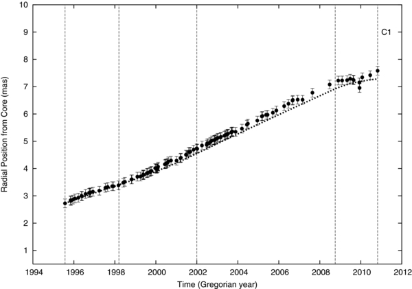
Figure 2. C1 component observed radial distance from core vs. time. The dotted line represents a model for which Lorentz factor, viewing angle, and intrinsic flux density are allowed to vary. The vertical dashed lines show the time intervals used in the modeling. There is a noticeable change in speed around 1998.
Download figure:
Standard image High-resolution image
Figure 3. C5 component observed radial distance from core vs. time. The dotted line represents a model for which Lorentz factor, viewing angle, and intrinsic flux density are allowed to vary. The dashed vertical lines show the time intervals used in the modeling. Clearly this component is undergoing complex motion (rapid increases and decreases in apparent speed), especially visible from 2002.5 to 2005.
Download figure:
Standard image High-resolution image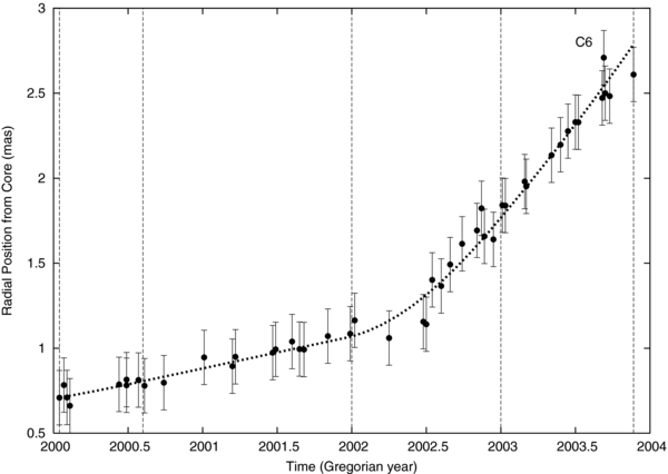
Figure 4. C6 component observed radial distance from core vs. time. The dotted line represents a model for which Lorentz factor, viewing angle, and intrinsic flux density are allowed to vary. The dashed vertical lines show the time intervals used in the modeling. The rapid increase in apparent speed goes from 5c to 40c.
Download figure:
Standard image High-resolution image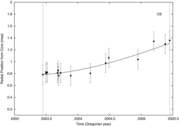
Figure 5. C8 component observed radial distance from core vs. time. The dotted line represents a model for which Lorentz factor, viewing angle, and intrinsic flux density are allowed to vary. The dashed vertical lines show the time intervals used in the modeling. This component increases its apparent speed from 1.4c to 12c
Download figure:
Standard image High-resolution imageKellermann & Owen (1988) aid in visualizing these results by plotting βapp versus ϑ for a set of different values of Γ.
We thus begin with these values from Equations (7) and (8), and search parameter space until χ2 is minimized (discussed below). The same time intervals are then used for the remainder of the fits (described below) for each component. For simplicity, we have chosen a linear dependence with time (in each interval) for each of these parameters. The results of these fits are given in Table 1.
Table 1. Model Parameters
| Component | Start Time, t1 | End Time, t2 | Γ1 | Γ2 | ϑt1 | ϑt2 | δt1 | δt2 | Ft1 | Ft2 |
|---|---|---|---|---|---|---|---|---|---|---|
| (rad) | (rad) | (Jy) | (Jy) | |||||||
| (1) | (2) | (3) | (4) | (5) | (6) | (7) | (8) | (9) | (10) | (11) |
| C1 | 1995.57 | 1998.2 | 15.82 | 12.92 | 0.019 | 0.026 | 29.0 | 23.2 | 4.2 × 10⁻⁶ | 1.2 × 10⁻⁵ |
| 1998.2 | 2002.0 | 12.92 | 15.82 | 0.026 | 0.027 | 23.2 | 26.7 | 1.2 × 10⁻⁵ | 2.6 × 10⁻⁶ | |
| 2002.0 | 2008.75 | 15.82 | 15.82 | 0.027 | 0.025 | 26.7 | 27.3 | 2.6 × 10⁻⁶ | 1.5 × 10⁻⁷ | |
| 2008.75 | 2010.82 | 15.82 | 11.19 | 0.025 | 0.010 | 27.3.1 | 22.1 | 1.5 × 10⁻⁷ | 1.3 × 10⁻⁶ | |
| C5 | 1998.18 | 2000.5 | 35.36 | 35.36 | 0.005 | 0.006 | 68.6 | 67.7 | 6.5 × 10⁻⁷ | 3.0 × 10⁻⁷ |
| 2000.5 | 2002.0 | 35.36 | 35.36 | 0.006 | 0.004 | 67.7 | 69.3 | 3.0 × 10⁻⁷ | 1.8 × 10⁻⁷ | |
| 2002.0 | 2002.5 | 35.36 | 40.83 | 0.004 | 0.015 | 69.3 | 59.4 | 1.8 × 10⁻⁷ | 2.0 × 10⁻⁷ | |
| 2002.5 | 2003.75 | 40.83 | 31.63 | 0.015 | 0.009 | 59.4 | 58.5 | 2.0 × 10⁻⁷ | 1.7 × 10⁻⁷ | |
| 2003.75 | 2005.5 | 31.63 | 31.63 | 0.009 | 0.003 | 58.5 | 62.7 | 1.7 × 10⁻⁷ | 1.5 × 10⁻⁷ | |
| 2005.5 | 2009.6 | 31.63 | 35.36 | 0.003 | 0.008 | 62.7 | 65.5 | 1.5 × 10⁻⁷ | 5.9 × 10⁻⁸ | |
| 2009.6 | 2010.0 | 35.36 | 35.36 | 0.008 | 0.001 | 65.5 | 70.6 | 5.9 × 10⁻⁸ | 1.5 × 10⁻⁹ | |
| 2010.0 | 2010.82 | 35.36 | 31.63 | 0.001 | 0.001 | 70.6 | 63.2 | 1.5 × 10⁻⁹ | 4.5 × 10⁻⁸ | |
| C6 | 2000.04 | 2000.6 | 28.87 | 31.63 | 0.003 | 0.003 | 57.3 | 62.7 | 5.3 × 10⁻⁷ | 3.9 × 10⁻⁷ |
| 2000.6 | 2002.0 | 31.63 | 31.63 | 0.003 | 0.003 | 62.7 | 62.7 | 3.9 × 10⁻⁷ | 4.7 × 10⁻⁷ | |
| 2002.0 | 2003.0 | 31.63 | 35.36 | 0.003 | 0.019 | 62.7 | 48.7 | 4.7 × 10⁻⁷ | 3.8 × 10⁻⁷ | |
| 2003.0 | 2003.89 | 35.36 | 40.83 | 0.019 | 0.019 | 48.7 | 50.98 | 3.8 × 10⁻⁷ | 2.0 × 10⁻⁷ | |
| C8 | 2003.45 | 2005.4 | 9.55 | 11.96 | 0.008 | 0.088 | 18.9 | 11.4 | 1.5 × 10⁻⁵ | 1.1 × 10⁻⁵ |
Download table as: ASCIITypeset image
In this table, Column 1 refers to the component being considered. The parameters of the tested models are the bulk Lorentz factor, Γ, viewing angle, ϑ, and the intrinsic flux density (Fν, int). Columns 2 and 3 give the start and end times of the fitted intervals. Columns 4 and 5 give the starting and ending bulk Lorentz factors. Columns 6 and 7 give the starting and ending viewing angles. Columns 8 and 9 give the beginning and ending Doppler factors using Equation (4). Columns 10 and 11 give the beginning and ending intrinsic flux density values. The results of our χ2 analysis of these models are given in Table 2. Column 1 refers to the component being considered and Column 2 refers to the time-dependent quantity that is being fitted. The explanation and calculation of χ2 in Column 3 can be found in Chapter 13 of Press et al. (1986). The probability given in Column 4 is such that the model could lead to a χ2 value as poor as that calculated by chance. Generally speaking, very low probability values (<1 × 10⁻³) would indicate a poor fit. If the probability is given as 0, it is less than the lowest value that can be calculated by our χ2 routine. The number of degrees of freedom (dof) given in Column 5, as defined in Chapter 13 of Press et al. (1986), is also given in Table 2.
Table 2. χ2 Analysis
| Component | Parameter | χ2 | Probability | dof |
|---|---|---|---|---|
| (1) | (2) | (3) | (4) | (5) |
| C1 | Flux | 2442 | 0.0 | 107 |
| βapp | 3.83 | 1.0 | 102 | |
| C5 | Flux | 932 | 0.0 | 85 |
| βapp | 34 | 0.99 | 76 | |
| C6 | Flux | 697 | 0.0 | 41 |
| βapp | 12.05 | 0.99 | 36 | |
| C8 | Flux | 255 | 0.0 | 14 |
| βapp | 5.749 | 0.93 | 12 | |
Download table as: ASCIITypeset image
3.3. Theoretical Background
Though we leave the magnitude of intrinsic flux density as a free parameter in our model above, we can get a sense of whether or not our model results are realistic or at least partly explained if we consider a model such as the shocked jet model of Marscher & Gear (1985). We first consider that the intrinsic flux density of a homogeneous source is proportional to the electron energy normalization factor, K, and the magnetic field, B, in the following way:

where the relativistic electron energy distribution is defined by

and R is the radius of the jet.
In Marscher & Gear (1985), broadband flux variations are modeled by a shock passing through a relativistic jet. If we assume a plasma of relativistic electrons and subrelativistic protons with adiabatic index of 13/9 and if the compression ratio of the shock (in the strong shock limit) can be approximated as
then the energy normalization factor can be enhanced by a factor of ηξp − 1, where ξ is a constant factor by which the electron energies are enhanced. For the purposes of order-of-magnitude analysis, we can, as Marscher & Gear (1985) discuss, assume that ξ has a lower limit related to the compression ratio of η1/3. Similar considerations lead to a magnetic field enhancement of approximately (η2 + 1/2)1/2. We note that Γ' is the bulk Lorentz factor of the shocked medium as viewed from the un-shocked medium and can be assumed to have a value between approximately 1 and 2 (Marscher & Gear 1985).
However, we also need to take into consideration the radial decrease of electron density and magnetic field as the shock progresses down the jet. First, we can assume that these quantities decrease following a power law

and assuming that the jet flow is adiabatic (Marscher & Gear 1985), then
and also

and

where, as before, R refers to the radius of the jet, r refers to the distance down the jet from the apex, and r0 is a reference point some radial distance from the apex of the jet, and usually taken to be physically related to the observed VLBI core. For a conical jet,  = 1 and a = tanλ, where λ refers to the jet opening angle.
Combining this with the flux density dependence on the aforementioned parameters in Equation (9), we can then show that the optically thin flux density will be proportional to the radius in the following way:

where

If we assume, as do Marscher & Gear (1985), that the distance down the jet can be determined observationally based on the observed progression of the component, and inferred velocity and viewing angle, then we can further use
Substituting into Equation (16), we get
where tobs refers to the time of observation and tej refers to the time of ejection of the component from the core. If we can then compare the expected radial amplification factor between the two intervals, and then multiply by the shock amplification factor discussed above, we arrive at a new combined amplification factor, Af:
We consider this model in interpreting our results in our discussion in Section 4 below.
3.4. Summary of Proper Motion and Flux Density Observations by Component
Here we summarize the details of what is seen for each component.
C1. In Figure 2, we see that the plot of radial distance from the core versus time shows a significant transition in 1998 due to an increase in βapp (the slope of this diagram) from near 8 to as high as 11 in 2003, decreasing again thereafter. The 1998 event has previously been interpreted as due to an impulse acceleration (Homan et al. 2003) related to a sudden bend in the jet. In Figure 6, we see that the observed flux density is primarily decreasing, which we have modeled as being due to a decrease of intrinsic flux density (Table 1). The relativistic Doppler factor, δ, is also primarily decreasing over the period of observations (with some small fluctuations; see Table 1), contributing to the decrease in observed flux density (Figure 6).
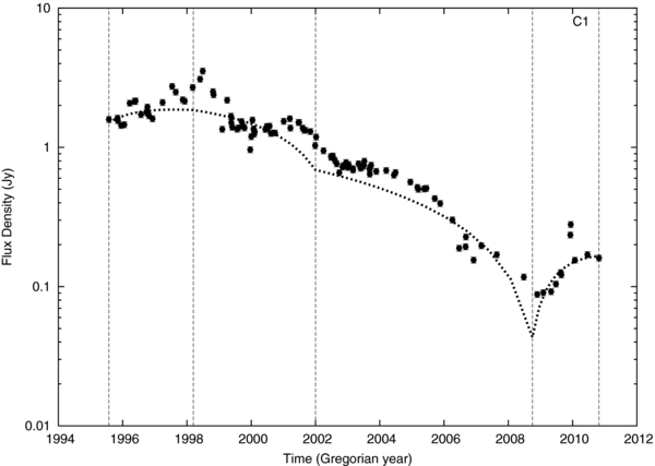
Figure 6. C1 component observed flux density vs. time. The dotted line represents a model for which Lorentz factor, viewing angle, and intrinsic flux density are allowed to vary. The dashed vertical line show the time intervals used for the modeling.
Download figure:
Standard image High-resolution imageC5. From Figure 3, we can see that this source exhibits very complex motion, especially between 2002.5 and 2005.5, during which time we see a sudden increase in apparent speed, βapp, followed by a decrease. Though proper motion, μ (and thus βapp), is generally well fitted for all components, C5 clearly has the poorest fit. These results could indicate a relatively fast-moving unresolved component that is leading us to misinterpret the radial distance curve around 2002.5 to 2005.5. The observed flux density (Figure 7) is decreasing during the range of observations, primarily due to a decrease in intrinsic flux density.
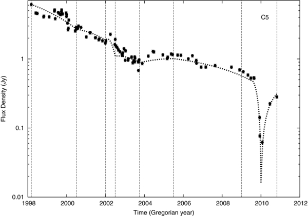
Figure 7. C5 component observed flux density vs. time. The dotted line represents a model for which Lorentz factor, viewing angle, and intrinsic flux density are allowed to vary. The dashed vertical lines show the time intervals used in the modeling.
Download figure:
Standard image High-resolution imageC6. The visible dramatic change in the motion of this component (Figure 4) is best explained by both an increase in Γ from 29 to 41 and an increase in viewing angle from 02 to 11, accounting for the change in βapp from 5c in 2002.0 to 40c in 2003.9. The observed flux density (Figure 8) is decreasing during this time, which we have modeled as being caused mainly by a decrease in intrinsic flux density (Table 1).
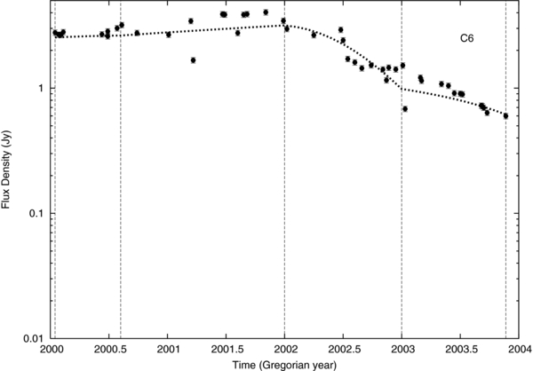
Figure 8. C6 component observed flux density vs. time. The dotted line represents a model for which Lorentz factor, viewing angle, and intrinsic flux density are allowed to vary. The dashed vertical lines show the time intervals used in the modeling.
Download figure:
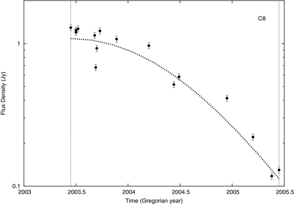
Standard image High-resolution imageC8. The increase in slope of the plot in Figure 5 indicates that this component has gone from an apparent speed of 1.4c to 12c due to a dramatic change in viewing angle from 05 to 50 and an increase in Lorentz factor from Γ = 9 to 12. The observed flux density (Figure 9) is decreasing steadily during this same time frame, which we have modeled as being caused by a decrease in Doppler beaming factor, δ, from approximately 19 down to near 11 (see Table 1), while the intrinsic flux density remains roughly constant (see Table 1).
Figure 9. C8 component observed flux density vs. time. The dotted line represents a model for which Lorentz factor, viewing angle, and intrinsic flux density are allowed to vary. The dashed vertical lines show the time intervals used in the modeling.
Download figure:
Standard image High-resolution image
3.5. Using Accelerations to Constrain Values of Kinematic Parameters
We can follow up this analysis by additionally constraining Lorentz factors and viewing angles with theoretical modeling of the measured accelerations. After fitting Gaussian circular models to the (u, v) data using the MODELFIT routine within DIFMAP we have determined the positions of distinct features as a function of time. Following Homan et al. (2001), we have first determined the x and y positions (relative right ascension and declination, respectively) of each robust modeled component, and then used the LFIT fitting routine from Numerical Recipes (Press et al. 1986) to parameterize the x and y positions in terms of angular velocity and acceleration in the following way:
Here, μx and μy refer to the proper motions in the x and y directions, t0 is the time of component ejection, and tmid is the midpoint of the time span of the observations of the given component.
The accelerations can then be transformed to a coordinate system with components perpendicular and parallel to the radial motion (if this direction is presumed constant):


Here, ϕ refers to the angle between the velocity vector and the y-axis.
In this context, the parallel accelerations correspond to either a speeding up or a slowing down in the radial direction or a change in the angle to the line of sight (or both), and the perpendicular accelerations are those that cause bending in the azimuthal direction (in reference to the line of sight). We caution readers not to confuse this geometry with the geometry of the jet itself. A more detailed description, including diagrams, can be found in Homan et al. (2009).
The uncertainties of the accelerations are calculated in a manner similar to that of Homan et al. (2001). That is, there are no initial assumptions regarding the uncertainties of the input component positions. Rather, the positions that go into the fit are initially weighted by unity, and then iteratively weighted by whichever uncertainty values are needed to bring the reduced χ2 of the fit down to approximately one. Though this method does not allow us to conclude that the assumed model is the correct one, the estimated uncertainties are valid if the model outlined above is the appropriate choice (Lister et al. 2009b).
We can determine the consistency of observed values with theoretically determined accelerations following the procedure of Homan et al. (2009). They use the following formulae to predict parallel and perpendicular accelerations and transform them into expressions for changes in the proper motion:
Here, β is the speed as a fraction of the speed of light,  is the time derivative of β, ϑ is the viewing angle,
  is the time derivative of this angle, and
  is the time derivative of the azimuthal angle relative to an axis along the direction of the viewing angle.
  and
and  refer to the parallel and perpendicular components of acceleration in angular units (mas yr−2), and μ is the proper motion in mas yr−1.
Understanding these formulae above requires some constraints on the time derivatives  ,
,  , and
, and  . These cannot be directly observed but further constraints can be put on these values by examining the proper motion diagrams (Figures 2–5) and light curves (Figures 6–9), as we discussed above. To aid in the interpretation of the results we note that a non-zero perpendicular acceleration only corresponds to a bend of the component direction in the azimuthal direction, with respect to the radial velocity vector. There are no consequences for the bulk speed. Interpreting the parallel acceleration is more complex. In the limiting case for which
  (no changes in bulk speed), an increase in apparent parallel velocity can still occur if
  and β < cos ϑ or when
  and β > cos ϑ. For the limiting case of
  an increase in apparent velocity can still occur for
  . For the case of decreasing apparent velocity, the same relationships hold with a simple reversal of the inequality sign above for
  .
.
Using Equations (27) and (28) above, we determine that the predicted theoretical acceleration over the entire interval of observations is approximately equal to those observed if the values of the parameters in Equations (25) and (26) equal those presented in Table 3. In Table 3, Column 1 identifies the component being considered,  in Column 2 and σ∥ in Column 3 refer to the acceleration of proper motion in the direction parallel to the proper motion vector and the associated uncertainty.
  in Column 4 and σ⊥ in Column 5 refer to the acceleration of proper motion in the direction perpendicular to the proper motion vector and the associated uncertainty. t1 in Column 6 and t2 in Column 7 refer to the relevant time interval of the data being modeled, β in Column 8,
  in Column 9, ϑ in Column 10,
  in Column 11, and
  in Column 12 have the same meaning as in Equations (25) and (26) above. ϑ is taken to be the initial value from Table 1 and β is calculated from Γ (given in Table 1) using Equation (3).
Table 3. Acceleration Model Parameters
| Component |  |
σ∥ |  |
σ⊥ | t1 | t2 | β |  |
ϑ |  |
 |
|---|---|---|---|---|---|---|---|---|---|---|---|
| (mas yr−1) | (mas yr−1) | (mas yr−1) | (mas yr−1) | (yr−1) | (rad yr−1) | (rad yr−1) | |||||
| (1) | (2) | (3) | (4) | (5) | (6) | (7) | (8) | (9) | (10) | (11) | (12) |
| C1 | 0.0004 | 0.0037 | 0.0130 | 0.0037 | 1995.57 | 2010.46 | 0.998 | 2.0 × 10⁻⁸ | 0.019 | −9.3× 10⁻⁸ | 1.6 × 10⁻⁴ |
| C5 | −0.0189 | 0.0042 | −0.0001 | 0.0042 | 1999.37 | 2010.46 | 0.9996 | −5.0 × 10⁻⁹ | 0.005 | −1.0 × 10⁻⁷ | −1.8 × 10⁻⁷ |
| C6 | 0.2916 | 0.0290 | 0.0284 | 0.0290 | 2000.04 | 2003.89 | 0.9994 | 9.9 × 10⁻⁷ | 0.003 | 1.5 × 10⁻⁷ | 1.7 × 10⁻⁴ |
| C8 | 0.1245 | 0.0755 | 0.3821 | 0.0755 | 2003.45 | 2005.45 | 0.9945 | 5.3 × 10⁻⁵ | 0.008 | 1.0 × 10⁻⁴ | 6.7× 10⁻² |
Download table as: ASCIITypeset image
3.6. Consistency between Two Methods
We can check for some consistency between the methods in Sections 3.1, 3.2, and 3.5 in the following manner. Using the results in Section 3.1 (Table 1) we can estimate the overall change in viewing angle, Δϑ, for each component. We can then divide by the change in time, Δt, to estimate  determined in Section 3.3; however, we must correct for the relativistic motion of the component into the line of sight and divide the observed time interval by (1 + z)(1 − βcos ϑ) now to get Δt'. We can estimate
  in similar manner. There are some caveats. For instance, both β and ϑ may be changing rapidly over the range of observations. Therefore, the values used for these quantities in further calculations are likely only to be rough averages over the entire time range of our observations. Performing these estimations leads to mixed results. For instance, for C5, we estimate Δϑ/Δt' to be approximately −2.3 × 10⁻⁷ rad yr−1. As compared to
  in Table 3, there is a 130% difference. In repeating for Δβ/Δt', we estimate −5.8 × 10⁻⁹. As compared to
  in Table 3, there is a 16% difference. However, this is the case with the best agreement between these methods. At the other extreme, for C1, we estimate (Δϑ/Δt') = 2.5 × 10⁻⁶, which has a 2600% difference with
  in Table 3. Comparison of (Δβ/Δt') = −5.6 × 10⁻⁷ with
  shows a 2900% difference. Though the results are mixed, they are promising in that they can be self-consistently used to make a first estimate of
  and
and  , to be refined by the methods in Section 3.5. Such a method may also be used to assist in rejecting our simple acceleration model, for cases such as C5, for which discrepancies are large.
4. DISCUSSION
We see above that there are a number of Lorentz factors associated with this jet, and that these Lorentz factors are changing over time. Though these results could potentially be explained by some variation of an underlying flow speed, an alternative is that we are seeing pattern speeds due to shocks moving through the jet. In particular, we see that C1 and C8 have overlapping values of Lorentz factor (in the range of about 9–16), and to some extent, viewing angles. In contrast, both C5 and C6 have overlapping Lorentz factor ranges, from 29 to 41. These may all be pattern speeds due to shocks, or possibly there can be a mixture of jet flow speed and pattern speed. Furthermore, both methods discussed in Section 3 are consistent with changing viewing angles for all components. As we discuss below, the variation of intrinsic flux density also seems consistent with this interpretation.
Above, we show that some of the intrinsic optically thin flux density variations of individual components could be as great as a factor of 430 (C5) over the entire time range. However, we only see up to a factor of 30 increase over a single time interval of a particular component and up to a factor of 39 decrease. We first explore whether the range of intrinsic flux density is consistent with what we might expect from a shocked jet, as presented in the previous section. We can use Equation (20) for comparison to two examples from our data. Both for components C1 and C5, we see that around the year 2010.0 (see Table 1) there was an increase of intrinsic flux density (by a factor of 9 for C1 and a factor of 30 for C5) and a simultaneous decrease in viewing angle. If we assume that Γ' is between 1 and 2, and assuming that = 0.5–1, b = 1–2, and p = 2–3, and n = 2.67–3.33 if the jet is adiabatic, we can then substitute in the values of β, cos ϑ, tej that are relevant for these components. For C1, we use Γ = 11.19–15.82 (β = 0.996–0.998), and ϑ from 06 to 15. During this time period, 2008.75–2010.82, Fν, int varies from 1.5 × 10⁻⁷ Jy to 1.3 × 10⁻⁶ Jy. The ejection time of this component from the core was 1987.8 (Lister et al. 2009b). We predict a range of amplifications of intrinsic flux density of approximately 36–210 (16–1100 if we relax the adiabatic assumption, and allow n to range from 2 to 5). For C5, we use Γ = 31.63–35.36 (β = 0.9995–0.9996), and ϑ is constant at 006. During this time period, 2010.0–2010.82, Fν, int varies from 1.5 × 10⁻⁹ Jy to 4.5 × 10⁻⁸ Jy. The ejection time from the core for this component was in 1997.36 (Lister et al. 2009b). We predict a range of amplifications of intrinsic flux density in this case of approximately 69–720 (73–1300 if we relax the adiabatic assumption and allow n to range from 2 to 5). Though even the low end of this range is higher than the level of variability that we actually observe, it is encouraging that the component with the lower predicted amplification factor also has the lowest observed magnitude of variability. The high end of the range of amplification values for both cases presented here is as a result of the higher possible shock speeds. Clearly, the higher shock speeds (Γ' = 2 or higher) are ruled out. So, though some of the variations are consistent with such a shocked jet model, in detail, a more refined model would be needed to describe all of the time intervals.
Additionally, polarization observations of one component can further constrain values of Lorentz factor and viewing angle. The fractional linear polarization of component (C5) was approximately 40% for 2002.9 (Lister & Homan 2005). Because the electric field vectors are roughly parallel to the component motion direction, we know that the magnetic field must be perpendicular to the jet, as we would expect for a shock (Laing 1980). However, shock-ordered fields only appear ordered if they are being viewed from the side. Because we see a high level of field order from this component, we must be viewing somewhere close to 90° in the aberrated frame. A component being viewed at 90° in the aberrated frame must be moving close to the critical angle, β = cos ϑ, as can be seen by considering relativistic aberration of angles:
Here, ϑab refers to the viewing angle in the aberrated frame. For β = 0.9995–0.9997 (Γ = 31.63–40.83) this gives ϑ = 14–18, which is significantly larger than the ϑ = 05 − 09 derived for this time period and reported in Table 1.
5. CONCLUSIONS
Analysis of the proper motions of the superluminal components of 3C 279 indicates significant accelerations for four components in at least one of the two calculated directions of acceleration (parallel and perpendicular to the original component motion). We see over all the components studied here a range of Lorentz factors of Γ = 10–41, viewing angle with range ϑ = 01–50, and intrinsic flux density in the range Fν, int = 1.5 × 10⁻⁹–1.5 × 10⁻⁵ Jy. Considering the individual components, Lorentz factor varies from Γ = 12–16 for C1, Γ = 31–41 for C5, Γ = 29–41 for C6, and Γ = 9–12 for C8. These ranges indicate that we cannot be looking at a single underlying jet flow speed, but may be seeing separate pattern speeds from shocks moving through the jet, or a combination of flow speed and pattern speed. We see that the magnitude of variability of the intrinsic flux density is between about 1.4 (C8) and 430 (C5) and viewing angle is in the range 05–50 for C8, 01–09 for C5 (these last two have the largest range), and 06–15 (the smallest range) for C1. Modeling of the accelerations shows consistency with jet bending in the viewing angle direction, and in the direction azimuthal to the viewing angle. Though these results are consistent with a shocked jet model, a more detailed time-dependent model including bends in the jet would be needed to consider the specifics for each component. Since all four components have at least one direction of acceleration that is less than 3σ times the associated uncertainty, this may be further indication that a more refined model is needed.
However, it may be possible that blending of shocks moving at different speeds is partly causing these observed effects (Agudo et al. 2001). Polarization measurements of component C5 also indicate viewing angles somewhat larger than those determined by other means (about 14–18 from polarization and 05–09 from kinematics and flux variation) during one epoch (2002.9).
The authors all acknowledge many insightful and helpful comments from the anonymous referee.
S.D.B. acknowledges many helpful discussions with D. C. Homan, M. L. Lister, K. I. Kellermann, and Y. Y. Kovalev. S.D.B. also acknowledges several Summer Faculty Fellowship grants from Hampden-Sydney College, as well as support from the Visiting Scientist Program at the National Radio Astronomy Observatory.
E.R. acknowledges partial support by the Spanish MICINN through grant AYA2009-13036-C02-02. E.R. and C.M.F. acknowledge support from the COST action MP0905 "Black Holes in a Violent Universe." C.M.F. has been supported by the International Max Planck Research School for Astronomy and Astrophysics.
This research has made use of data from the MOJAVE database that is maintained by the MOJAVE team (Lister et al. 2009a).
This work has made use of data obtained from the National Radio Astronomy Observatory's Very Long Baseline Array and its public archive. The National Radio Astronomy Observatory is a facility of the National Science Foundation operated under a cooperative agreement by Associated Universities, Incorporated.