


ABSTRACT
We report the orbital distribution of the trans-Neptunian comets discovered during the first discovery year of the Canada–France Ecliptic Plane Survey (CFEPS). CFEPS is a Kuiper Belt object survey based on observations acquired by the Very Wide component of the Canada–France–Hawaii Telescope Legacy Survey (LS-VW). The first year's detections consist of 73 Kuiper Belt objects, 55 of which have now been tracked for three years or more, providing precise orbits. Although this sample size is small compared to the world-wide inventory, because we have an absolutely calibrated and extremely well-characterized survey (with known pointing history) we are able to de-bias our observed population and make unbiased statements about the intrinsic orbital distribution of the Kuiper Belt. By applying the (publically available) CFEPS Survey Simulator to models of the true orbital distribution and comparing the resulting simulated detections to the actual detections made by the survey, we are able to rule out several hypothesized Kuiper Belt object orbit distributions. We find that the main classical belt's so-called 'cold' component is confined in semimajor axis (a) and eccentricity (e) compared to the more extended "hot" component; the cold component is confined to lower e and does not stretch all the way out to the 2:1 resonance but rather depletes quickly beyond a = 45 AU. For the cold main classical belt population we find a robust population estimate of N(Hg < 10) = 50 ± 5 × 10³ and find that the hot component of the main classical belt represents ∼60% of the total population. The inner classical belt (sunward of the 3:2 mean-motion resonance) has a population of roughly 2000 trans-Neptunian objects with absolute magnitudes Hg < 10, and may not share the inclination distribution of the main classical belt. We also find that the plutino population lacks a cold low-inclination component, and so, the population is somewhat larger than recent estimates; our analysis shows a plutino population of N(Hg < 10)∼ 25+25−12 × 103compared to our estimate of the size of main classical Kuiper Belt population of N(Hg < 10) ∼ (126+50−46) × 103.
Export citation and abstract BibTeX RIS
1. INTRODUCTION
In 1949 Edgeworth, and in 1951 Kuiper, postulated the existence of a debris disk beyond the orbit of Neptune. Their expectation was based on the hypothesis that material in this zone had likely not formed into large planets (Irwin et al. 1995). Pluto had been discovered two decades earlier but was not recognized at the time as a large member of this hypothesized disk of debris. Several decades would pass before a few researchers began to search in earnest for small bodies beyond Neptune. These searches were motivated by the realization that the discovery and study of the orbits and properties of the members of such a debris disk could provide a rich understanding of the formation and evolution of the outer solar system. For example, the objects may be composed of some of the most pristine materials left over from the formation of the solar system. Also, a measure of the mass and orbital distribution of objects in this zone of the solar system could confirm this region as the source of short period comets.
The discovery of the first object recognized to be a member of the outer solar system debris disk, 1992 QB1 (Jewitt et al. 1992), led to an avalanche of searches and discoveries. In a mere 15 years, observers have discovered over 1200 small trans-Neptunian bodies. A gold rush of discovery compared with the case of asteroids, where over 130 years were needed to discover a comparable number; only four asteroids were known for over 44 years after the discovery of the first, Ceres. Some of these outer solar system bodies are estimated to be larger than Pluto, which itself is now understood to be one of the largest and closest of the Kuiper Belt objects (KBOs).
1.1. Initial Impression of the KBO Orbit Distribution; Influence on Survey Progress
Jewitt et al. (1996) provided one of the first estimates of the size and shape of the Kuiper Belt. In this early work they considered the biases against detections of high-inclination objects and determined that the intrinsic width of the Kuiper Belt is likely around ∼30° FWHM, much broader than anticipated. As surveys of the Kuiper Belt have continued, observers are becoming more aware that a correct assessment of all observational bias is critical if one is to correctly measure the intrinsic distribution of material in the distant solar system. Over the past decade, a number of surveys (Jewitt et al. 1998; Larsen et al. 2001; Trujillo et al. 2001; Gladman et al. 2001; Allen et al. 2002; Jones et al. 2006) have further refined these statistics and Elliot et al. (2005) provide the survey of the Kuiper Belt with the largest number of detected and tracked objects. A compilation of the detection rates and subpopulation estimates from these KBO surveys can be found in the Kavelaars et al. (2008). These previous surveys have provided exciting insights into this region of the solar system.
The precise determination of a KBO orbit often requires an observational arc of many years in length. The long time commitment and frequent observations often lead to observational biases that are difficult to account for (see Jones et al. 2006; Kavelaars et al. 2008, for further details). A survey which desired to provide a detailed and accurate description of the underlying Kuiper Belt population must pay very close attention to survey characterization. In the Canada-France-Ecliptic Plane Survey (CFEPS) we have taken great pains to characterize and track the survey detections so that one can make robust statements regarding the underlying orbital distribution in the Kuiper Belt. In the CFEPS project we have tracked ∼85% of our characterized detections (see Section 3.1), to-date this is the highest fraction of tracked objects for any KBO survey. Though the sample we report here is only ∼5% of the world inventory of KBOs with known orbits, we are able to make a number of interesting and new statements regarding the intrinsic orbital structure of the Kuiper Belt region because of our careful attention to the survey characteristics.
In Sections 2 and 3, we describe the observations and characterization of the CFEPS L3 KBO sample. In Section 4, we explain the use of our survey simulator and statistical methods and in Section 5 we describe our parametrized models of the KBO orbit distribution and provide estimates of the total number of objects in each subpopulation modeled.
2. OBSERVATIONS
The CFEPS project uses images acquired by the Very Wide component of the Canada-France-Hawaii Telescope Legacy Survey (LS-VW) for discovery and a large fraction of the follow-up imaging. LS-VW observations where made using the one degree field of view of the CFHT MegaPrime camera. CFHT MegaPrime provides well sampled images with a typical image quality of 0.7–0.9 arcsec FWHM. The LS-VW observations were designed to maximize the opportunity to discover and track trans-Neptunian objects (TNOs) while providing multi-filter, multi-epoch imaging that could be used to pursue secondary science goals. The LS-VW project was awarded 50 nights per year on CFHT to allow observations to cover a sky area of about 1300 square degrees along the ecliptic (the entire sky within 2 degrees of the ecliptic plane and more than 10 degrees from the galactic plane). The survey started in 2003 March and was severely hampered by technical and weather problems for the first 3 semesters of operation. In 2005 May the Scientific Advisory Committee of the CFHT, reacting to a lower than anticipated observing efficiency of the CFHT Legacy Survey, ramped down the LS-VW observations such that only 400 of the originally anticipated 1300 square degrees were covered.
This manuscript details the observational campaign and analysis arising from those KBOs detected in the first calendar year of the LS-VW project. These KBOs (discovered in ∼94 square degrees of imaging in 2003) are referred to as the L3 data release because our internal designation of these detections all begin with the string "L3".
Many of the KBOs recorded in the Minor Planet Center (MPC) database lack precise orbital elements and all contain biases, some of which are hidden. These biases often result in misinterpretation of the orbital distributions recorded in the MPC lists. The CFEPS observing strategy was developed with the goal of providing a set of high-quality KBO orbits free of tracking/ephemeris bias. Our discovery and followup program, coupled to "data releases" that provide only high-quality orbits, is specifically designed to reduce the biases present in the main MPC listing. LS-VW observations were made on at least six separate nights, with about fifteen separate observations of each field over the course of 3–4 years. A summary of our observing sequence is given below, a complete description of our observing strategy and logic is presented in Jones et al. (2006).
- Discovery: a set of 3 observations, separated by approximately 1 hr, targeting fields within 15° of opposition to allow detection of solar system objects via their reflex sky motion.
- Nailing: a single observation a few nights before or after the discovery triplet. These observations provided confirmation of the discovery observations.
- Checkup: a second set of three exposures. These observations are made when the field is at solar elongation between 125 and 110 degrees to avoid confusion with main-belt asteroids (see Figure 1). These observations provide the required sky motion arc so that ephemeris predictions a year later have uncertainty of less than one-degree of arc and reducing the chances of introducing ephemeris biases into our catalog.
- Recovery: a triplet of observations made when the field returns to opposition, coupled with a second Nailing observation. These observations provide an enormous improvement to the ephemeris of outer solar system objects and secure their positions for continued monitoring.
- Refinement: a final triplet of observations taken two years after discovery, providing orbital refinement to ⩽0.1% relative accuracy. For some objects additional observations were acquired three or even four years after discovery to provide needed improvements in the astrometry when fine orbital details are desired (to determine resonant libration, for example).

Figure 1. Angular rates of motion for objects on circular ecliptic-plane orbits with semimajor axis near the asteroid belt (dash lines show rates for objects at 2 and 6 AU) and the Kuiper Belt (dotted lines show rates of motion of objects at 30 and 100 AU). At solar elongation of ∼140° KBOs and main belt asteroids have similar angular rates of motion (gray area of plot), observing at elongation between 125° and 155° results in confusion between asteroids and KBOs in recovery observations.
Download figure:
Standard image High-resolution imageThe LS-VW CFHT MegaPrime observations imaged a grid of pointings using the g', r', and i' filters (Magnier & Cuillandre 2004). Fields, not KBO ephemerides, were targeted in the pre-refinement stages of this survey. The observing strategy ensures that our tracking observations are free of "ephemeris biases": orbit distribution biases induced by assuming orbits of the KBOs discovered in each field (see Kavelaars et al. 2008; Parker et al. 2007). Using a pointing-grid and ensuring that each field was observed in each filter enhanced the legacy value of the observations by providing imaging data to a broad range of astronomical projects.
Tables 1 and 2 provide a summary of the area, field geometry, filter coverage, exposure time, image quality and flux limits of the LS-VW observations and Figure 2 presents the geometry of a typical LS-VW observing block. Flux limits were determined by added artificial sources, with a range of fluxes and reflex motions, into the original images and determining the fraction of artificial sources detected by our detection pipeline (see Jones et al. 2006, for details).

Figure 2. Geometry of the sky-pointings for the L3q block. For each object the discovery position (2003 August 31) is shown as an open circle at the start of a line with the predicted location at (pre)checkup (2003 June 22) and recovery (2004 August 10) shown as open circles and large dots connected to the initial discovery location. The dashed line indicates the invariable plane while the dotted line indicates the location of the ecliptic plane. These 4 × 4 blocks resulted in very little loss due to north/south motion of the targets (little inclination dependence in the tracking success) but the eastern most KBOs drift off the coverage by the time of first opposition recovery (close-in objects could be lost preferentially). For these blocks we programmed our recovery observations with an additional column of fields along the eastern edge of the discovery block (shown in gray) and removed the western-most column of discovery fields. The object in the south-east of the patch, with a large error ellipse (l3q07), was lost at checkup and did not appear in the recovery observations, this target is also the faintest KBO in the L3q block and is faintward of the characterization limit of this block (see Table 3). The target in the northeast of the field (l3q05) should have appeared in the recovery observations but was not found, this target is part of the characterized sample for the L3q block and may have been lost off the north end of the recovery patch.
Download figure:
Standard image High-resolution imageTable 1. Summary of Field Positions and Detections
| Detections | Geometry | Limit | ||||||
|---|---|---|---|---|---|---|---|---|
| Block | R.A. (hrs) | Decl. (deg) | Fill Factor | Disc. | Tracked | DEG | DEG | gAB |
| L3f | 12:42 | −04:33 | 0.80 | 4 | 3 | 4 × 4 | 23.75 | |
| L3h | 13:03 | −06:48 | 0.81 | 20 | 12 | 4 × 4 | 24.45 | |
| L3q | 22:01 | −12:04 | 0.89 | 9 | 7 | 4 × 4 | 24.08 | |
| L3s | 19:43 | −01:20 | 0.87 | 6 | 6 | 14 × 1 | 23.95 | |
| L3w | 04:33 | 22:21 | 0.87 | 19 | 14 | 16 × 1 | 24.25 | |
| L3y | 07:30 | 21:48 | 0.85 | 15 | 13 | 4 × 4 | 24.08 | |
| Total | 73 | 55 | 94 sqr. deg. | |||||
Notes. Field centers. R.A./Decl. is the approximate center of the field. Fill Factor is the fraction of sky covered by the mosaic and useful for KBO searching. gAB refers to the g-band AB scale of the SDSS photometric system.
Download table as: ASCIITypeset image
Table 2. Summary of LS-VW Observations
| Date | Filter | Exposure Time (s) | Median FWHM (arcsec) |
|---|---|---|---|
| L3f | |||
| 2003 Mar 24 | G.MP9401a | 140 | 0.91 |
| 2003 Mar 27 | G.MP9401b | 140 | 1.0 |
| 2003 May 27 | R.MP9601a | 140 | 0.80 |
| 2003 Jun 6 | R.MP9601a | 140 | 0.90 |
| 2004 Mar 20 | G.MP9401a | 90 | 1.04 |
| L3h | |||
| 2003 Apr 26 | R.MP9601a | 140 | 0.84 |
| 2003 May 30 | R.MP9601b | 140 | 1.05 |
| 2004 Mar 20 | G.MP9401a | 75 | 0.80 |
| L3q | |||
| 2003 Jun 22 | I.MP9701a | 160 | 0.89 |
| 2003 Aug 31 | G.MP9401a | 90 | 0.89 |
| 2004 Aug 10 | R.MP9601a | 110 | 0.79 |
| L3s | |||
| 2003 Sep 23 | G.MP9401a | 70 | 0.89 |
| 2003 Nov 22 | I.MP9701a | 180 | 0.89 |
| 2004 Sep 12 | R.MP9601a | 110 | 0.83 |
| L3w | |||
| 2003 Oct 3 | I.MP9701a | 180 | 0.57 |
| 2003 Dec 16 | G.MP9401a | 90 | 0.93 |
| 2004 Nov 20 | R.MP9601b | 110 | 0.67 |
| L3y | |||
| 2003 Dec 24 | G.MP9401a | 75 | 0.79 |
| 2003 Dec 25 | G.MP9401b | 90 | 0.90 |
| 2005 Jan 6 | R.MP9601a | 110 | 0.88 |
| 2005 Jan 8 | R.MP9601a | 110 | 0.90 |
| 2005 Jan 15 | R.MP9601b | 110 | 0.90 |
Notes. The flux limit represents the magnitude above which greater than 40% of artificial sources where detected by our moving object pipeline (see Jones et al. 2006). aNight was photometric. bNight was not photometric.
Download table as: ASCIITypeset image
We experimented with conducting the discovery observations in the g' and r' filters, eventually standardizing on conducting all discovery observations in g'. Table 2 provides a detailed accounting of the relevant observational parameters of each block. The observational data acquired as part of the LS-VW are publicly available from the Canadian Astronomical Data Center.11
Exposure times were chosen to ensure a limiting magnitude (see Table 2) of mg ∼ 24, resulting in about one KBO detection per one square-degree FOV of the CFHT MegaPrime camera. This depth ensured that the discovered objects would be bright enough to permit tracking observations from telescopes with apertures as small as two meters diameter while maintaining a reasonable duty cycle per discovery field. To achieve this depth we elected to acquire 70 s exposures through the CFHT MegaPrime g' filter; sufficient to provide S/N ∼8 on  point sources in median (FWHM ∼ 0
 8) CFHT seeing (
 ).
).
Object motion was detected by re-observing each field three times with a minimum time separation of 30 minutes between exposures. To ease implementation within the CFHT queue system we programmed our observations in sequences such that the exposure length plus overhead between iterations provided the required temporal sampling. Given the expected overhead of 40 s per exposure and the 70 s exposure time, and the desire for at least 30 minutes between repeated exposures requires approximately 16 fields to be observed per cycle. We refer to each of these groups of ∼16 fields as an observation "block."
Checkup observations were used to eliminate confusion in orbit linkages between discovery and recovery. These off-opposition observations also greatly reduce orbital uncertainties in a multi-opposition orbit. Checkup observations target the same pointing grid as the discovery observations, occurring either in the months before (pre-checkup) or following (checkup) the block's passage through opposition. The ephemeris uncertainty for KBOs with only a one day arc (based on our discovery and nailing observations a few months before or after checkup) can be quite large (see Jones et al. 2006); to avoid confusion with main-belt asteroids, we ensured that all check-up fields were observed between solar elongation of 110 and 125 degrees (see Figure 1). Given this narrow range of elongation and our desire to keep all the fields observable over a minimum of 5 nights per dark run, we were restricted to field geometries that occupied no more than ∼15° of RA. Simultaneously, we maximized the R.A. size of each patch, in order to minimize the number of objects that sheared out of the field of view between discovery and checkup. Four of the L3 patches are roughly square R.A./decl. patches, (see Figure 2 for example) while two were observed as long strips. The geometry and central R.A./decl. of each of the six L3 blocks is given in Table 1.
2.1. Longitude Coverage
Observations where acquired as part of a queue-scheduled survey at the CFHT. Our fields were chosen to lie within 2 degrees of the ecliptic plane and the CFHT QSO (queue service observer) imaged those fields that were at opposition whenever our priority on the facility was higher than that of competing programs. This "pressure" balancing approach to the initial discovery observations resulted in about one "block" of observations per CFHT queue observing session (nominally the 7 days leading and trailing the new moon). As a result, the CFEPS sky coverage will span nearly the entire R.A. range with breaks near the galactic plane crossings (where we did not request observations) and at locations of very high queue pressure (typically May and October). The sky coverage of our L3 release is 94 square degrees (see Table 1)
3. SAMPLE CHARACTERIZATION
Each of the discovery blocks listed in Table 1 was searched for KBOs using our Moving Object Pipeline (MOP; see Petit et al. 2004). The detection flux limit (above which 40% of all artificial sources where recovered by the MOP) for each field is listed in Table 2, along with information about the filter sequencing.
TNOs detected in each of the discovery images are given a provisional CFEPS designation of lower-case letter "l" followed by the number 3 (indicating detection in 2003) followed by the letter of the block in which the detection occurred (each block is given a letter corresponding to the two-week period during which the discovery observations were made, similar to the MPC provisional designation system) finally an odometer number is added which counts up the number of KBOs detected in the block.
The provisional lower-case "l" is switched to an "L" once an object has been tracked to the "Checkup" phase, such objects are more likely to be recoverable in the second opposition (Parker et al. 2007). The 73 KBOs that received an "l" (14) or "L" (59) designation constitute our discovery sample. Other KBOs, such as 2004 XR190 (a.k.a. Buffy, Allen et al. 2006), discovered during tracking observations, are not included in our modeling samples and are reported to the MPC. Only those KBOs discovered in those images that we designate as our "discovery" images are considered as part of our survey sample. We then searched the MPC for objects at the same R.A./decl. location and any object which could be linked with a previously detected KBO was given the suffix designation PD. For example, the object L3q02PD was detected in the Legacy Survey data taken in the 17th two-week interval of 2003, and is a previously known KBO (2001 QB298).
3.1. Photometry and Detection Efficiency
The LS-VW observations are acquired as part of the CFHT queue system. For each field observed on a photometric night the CFHT QSO provides calibrated images using their ELIXIR processing software (Magnier & Cuillandre 2004). Our photometry is reported in the AB zero-point system defined by ELIXIR combined with an average color term for the camera run of the observation. All of the CFEPS discovery observations were acquired in photometric conditions. Using differential aperture photometry we measure the total flux for each of our detected objects on all photometric nights and these fluxes are reported in Table 3.
Table 3. Object Fluxes
| Object | g | σg | Ng | r | σr | Nr | i | σi | Ni |
|---|---|---|---|---|---|---|---|---|---|
| L3f01 | 23.46 | 0.03 | 3 | 23.12 | 0.08 | 3 | ⋅⋅⋅ | ⋅⋅⋅ | ⋅⋅⋅ |
| L3f02a | 23.97 | 0.06 | 3 | 23.41 | 0.18 | 3 | ⋅⋅⋅ | ⋅⋅⋅ | ⋅⋅⋅ |
| L3f04PD | 22.58 | 0.01 | 3 | ⋅⋅⋅ | ⋅⋅⋅ | ⋅⋅⋅ | ⋅⋅⋅ | ⋅⋅⋅ | ⋅⋅⋅ |
| L3h01 | 23.83 | 0.14 | 4 | 23.03 | 0.06 | 3 | ⋅⋅⋅ | ⋅⋅⋅ | ⋅⋅⋅ |
| L3h04 | 24.32 | 0.08 | 4 | 23.68 | 0.07 | 4 | ⋅⋅⋅ | ⋅⋅⋅ | ⋅⋅⋅ |
| L3h05 | 24.69 | 0.32 | 3 | 23.47 | 0.08 | 4 | ⋅⋅⋅ | ⋅⋅⋅ | ⋅⋅⋅ |
| L3h06a | ⋅⋅⋅ | ⋅⋅⋅ | ⋅⋅⋅ | 23.99 | 0.17 | 4 | ⋅⋅⋅ | ⋅⋅⋅ | ⋅⋅⋅ |
| L3h08 | ⋅⋅⋅ | ⋅⋅⋅ | ⋅⋅⋅ | 23.36 | 0.11 | 4 | ⋅⋅⋅ | ⋅⋅⋅ | ⋅⋅⋅ |
| L3h09 | 22.71 | 0.02 | 3 | 22.10 | 0.02 | 4 | ⋅⋅⋅ | ⋅⋅⋅ | ⋅⋅⋅ |
| L3h10b | ⋅⋅⋅ | ⋅⋅⋅ | ⋅⋅⋅ | 22.88 | 0.06 | 4 | ⋅⋅⋅ | ⋅⋅⋅ | ⋅⋅⋅ |
| L3h11 | 23.44 | 0.08 | 7 | 23.13 | 0.06 | 3 | ⋅⋅⋅ | ⋅⋅⋅ | ⋅⋅⋅ |
| L3h13 | 23.72 | 0.05 | 4 | 23.14 | 0.06 | 4 | ⋅⋅⋅ | ⋅⋅⋅ | ⋅⋅⋅ |
| L3h14 | 23.27 | 0.09 | 3 | 22.95 | 0.07 | 4 | ⋅⋅⋅ | ⋅⋅⋅ | ⋅⋅⋅ |
| L3h15b | ⋅⋅⋅ | ⋅⋅⋅ | ⋅⋅⋅ | 23.80 | 0.16 | 4 | ⋅⋅⋅ | ⋅⋅⋅ | ⋅⋅⋅ |
| L3h16b | ⋅⋅⋅ | ⋅⋅⋅ | ⋅⋅⋅ | 23.41 | 0.07 | 4 | ⋅⋅⋅ | ⋅⋅⋅ | ⋅⋅⋅ |
| L3h18 | 23.42 | 0.05 | 3 | 22.43 | 0.03 | 4 | ⋅⋅⋅ | ⋅⋅⋅ | ⋅⋅⋅ |
| L3h19 | ⋅⋅⋅ | ⋅⋅⋅ | ⋅⋅⋅ | 23.65 | 0.11 | 7 | ⋅⋅⋅ | ⋅⋅⋅ | ⋅⋅⋅ |
| L3h20 | ⋅⋅⋅ | ⋅⋅⋅ | ⋅⋅⋅ | 23.01 | 0.06 | 4 | ⋅⋅⋅ | ⋅⋅⋅ | ⋅⋅⋅ |
| L3q01 | 23.89 | 0.12 | 3 | 22.96 | 0.10 | 3 | 22.76 | 0.21 | 3 |
| L3q02PD | 23.50 | 0.06 | 3 | 22.49 | 0.04 | 4 | 22.23 | 0.01 | 3 |
| L3q03 | 23.19 | 0.09 | 4 | 22.48 | 0.02 | 3 | 22.37 | 0.11 | 1 |
| L3q04PD | 24.15 | 0.22 | 4 | 23.31 | 0.07 | 4 | 23.10 | 0.09 | 3 |
| L3q06PD | 23.58 | 0.15 | 4 | ⋅⋅⋅ | ⋅⋅⋅ | ⋅⋅⋅ | ⋅⋅⋅ | ⋅⋅⋅ | ⋅⋅⋅ |
| L3q08PD | 23.67 | 0.10 | 3 | ⋅⋅⋅ | ⋅⋅⋅ | ⋅⋅⋅ | ⋅⋅⋅ | ⋅⋅⋅ | ⋅⋅⋅ |
| L3q09PD | 23.50 | 0.12 | 4 | ⋅⋅⋅ | ⋅⋅⋅ | ⋅⋅⋅ | ⋅⋅⋅ | ⋅⋅⋅ | ⋅⋅⋅ |
| L3s01 | 23.54 | 0.05 | 6 | ⋅⋅⋅ | ⋅⋅⋅ | ⋅⋅⋅ | 22.54 | 0.08 | 2 |
| L3s02 | 23.81 | 0.12 | 6 | 23.40 | 0.12 | 4 | 23.18 | 0.08 | 2 |
| L3s03 | 22.90 | 0.09 | 5 | ⋅⋅⋅ | ⋅⋅⋅ | ⋅⋅⋅ | 22.65 | 0.13 | 3 |
| L3s04a | 24.10 | 0.19 | 6 | ⋅⋅⋅ | ⋅⋅⋅ | ⋅⋅⋅ | ⋅⋅⋅ | ⋅⋅⋅ | ⋅⋅⋅ |
| L3s05 | 23.73 | 0.16 | 4 | ⋅⋅⋅ | ⋅⋅⋅ | ⋅⋅⋅ | 22.88 | 0.09 | 2 |
| L3s06 | 22.82 | 0.02 | 5 | ⋅⋅⋅ | ⋅⋅⋅ | ⋅⋅⋅ | 21.89 | 0.04 | 3 |
| L3w01 | 23.15 | 0.09 | 4 | ⋅⋅⋅ | ⋅⋅⋅ | ⋅⋅⋅ | ⋅⋅⋅ | ⋅⋅⋅ | ⋅⋅⋅ |
| L3w02 | 23.56 | 0.05 | 4 | 22.80 | 0.04 | 4 | 22.54 | 0.04 | 3 |
| L3w03 | 23.76 | 0.03 | 5 | 22.50 | 0.04 | 4 | ⋅⋅⋅ | ⋅⋅⋅ | ⋅⋅⋅ |
| L3w04 | 22.44 | 0.01 | 5 | 21.65 | 0.02 | 4 | 21.53 | 0.01 | 3 |
| L3w05 | 24.20 | 0.15 | 4 | 23.70 | 0.10 | 3 | 23.77 | 0.04 | 3 |
| L3w06 | 23.65 | 0.13 | 4 | 23.13 | 0.09 | 4 | ⋅⋅⋅ | ⋅⋅⋅ | ⋅⋅⋅ |
| L3w07 | 22.95 | 0.04 | 5 | ⋅⋅⋅ | ⋅⋅⋅ | ⋅⋅⋅ | 22.46 | 0.05 | 3 |
| L3w08 | 23.96 | 0.07 | 4 | ⋅⋅⋅ | ⋅⋅⋅ | ⋅⋅⋅ | 22.79 | 0.08 | 3 |
| L3w09 | 23.53 | 0.06 | 3 | 22.72 | 0.07 | 4 | ⋅⋅⋅ | ⋅⋅⋅ | ⋅⋅⋅ |
| L3w10 | 23.95 | 0.09 | 5 | 23.04 | 0.07 | 4 | 22.71 | 0.11 | 1 |
| L3w11 | 24.03 | 0.06 | 4 | 23.49 | 0.08 | 4 | 23.34 | 0.07 | 3 |
| L3w12a | 24.43 | 0.09 | 3 | ⋅⋅⋅ | ⋅⋅⋅ | ⋅⋅⋅ | 23.48 | 0.15 | 3 |
| L3w13a | 24.39 | 0.1 | 4 | 23.96 | 0.12 | 3 | ⋅⋅⋅ | ⋅⋅⋅ | ⋅⋅⋅ |
| L3w16 | 24.07 | 0.07 | 4 | ⋅⋅⋅ | ⋅⋅⋅ | ⋅⋅⋅ | 23.14 | 0.14 | 3 |
| L3w17a | 24.45 | 0.05 | 4 | ⋅⋅⋅ | ⋅⋅⋅ | ⋅⋅⋅ | 23.28 | 0.09 | 3 |
| L3y01 | 23.92 | 0.08 | 3 | 22.93 | 0.07 | 2 | ⋅⋅⋅ | ⋅⋅⋅ | ⋅⋅⋅ |
| L3y02 | 23.38 | 0.04 | 6 | 22.60 | 0.03 | 3 | ⋅⋅⋅ | ⋅⋅⋅ | ⋅⋅⋅ |
| L3y03 | 23.40 | 0.06 | 3 | 22.80 | 0.08 | 3 | ⋅⋅⋅ | ⋅⋅⋅ | ⋅⋅⋅ |
| L3y04a | 24.25 | 0.09 | 3 | 23.81 | 0.22 | 2 | ⋅⋅⋅ | ⋅⋅⋅ | ⋅⋅⋅ |
| L3y05 | 23.89 | 0.02 | 3 | 22.99 | 0.07 | 3 | ⋅⋅⋅ | ⋅⋅⋅ | ⋅⋅⋅ |
| L3y06 | 23.37 | 0.10 | 3 | ⋅⋅⋅ | ⋅⋅⋅ | ⋅⋅⋅ | ⋅⋅⋅ | ⋅⋅⋅ | ⋅⋅⋅ |
| L3y07 | 23.46 | 0.04 | 3 | 22.71 | 0.02 | 3 | ⋅⋅⋅ | ⋅⋅⋅ | ⋅⋅⋅ |
| L3y08a | 24.23 | 0.09 | 3 | 23.43 | 0.14 | 3 | ⋅⋅⋅ | ⋅⋅⋅ | ⋅⋅⋅ |
| L3y09 | 23.57 | 0.02 | 3 | 22.92 | 0.06 | 3 | ⋅⋅⋅ | ⋅⋅⋅ | ⋅⋅⋅ |
| L3y11 | 23.66 | 0.03 | 3 | 23.42 | 0.07 | 3 | ⋅⋅⋅ | ⋅⋅⋅ | ⋅⋅⋅ |
| L3y12PD | 21.73 | 0.02 | 3 | 20.79 | 0.02 | 3 | ⋅⋅⋅ | ⋅⋅⋅ | ⋅⋅⋅ |
| L3y14PD | 23.59 | 0.05 | 3 | 22.73 | 0.06 | 3 | ⋅⋅⋅ | ⋅⋅⋅ | ⋅⋅⋅ |
| L3y16 | 24.07 | 0.16 | 3 | 23.45 | 0.09 | 3 | ⋅⋅⋅ | ⋅⋅⋅ | ⋅⋅⋅ |
| l3f05b | 23.71 | 0.10 | 3 | ⋅⋅⋅ | ⋅⋅⋅ | ⋅⋅⋅ | ⋅⋅⋅ | ⋅⋅⋅ | ⋅⋅⋅ |
| l3h02a | ⋅⋅⋅ | ⋅⋅⋅ | ⋅⋅⋅ | 23.96 | 0.13 | 4 | ⋅⋅⋅ | ⋅⋅⋅ | ⋅⋅⋅ |
| l3h03a | ⋅⋅⋅ | ⋅⋅⋅ | ⋅⋅⋅ | 24.01 | 0.05 | 3 | ⋅⋅⋅ | ⋅⋅⋅ | ⋅⋅⋅ |
| l3h07a | ⋅⋅⋅ | ⋅⋅⋅ | ⋅⋅⋅ | 24.35 | 0.21 | 4 | ⋅⋅⋅ | ⋅⋅⋅ | ⋅⋅⋅ |
| l3h12a | ⋅⋅⋅ | ⋅⋅⋅ | ⋅⋅⋅ | 23.79 | 0.09 | 7 | ⋅⋅⋅ | ⋅⋅⋅ | ⋅⋅⋅ |
| l3h17a | ⋅⋅⋅ | ⋅⋅⋅ | ⋅⋅⋅ | 24.17 | 0.16 | 4 | ⋅⋅⋅ | ⋅⋅⋅ | ⋅⋅⋅ |
| l3q05b | 23.68 | 0.08 | 4 | ⋅⋅⋅ | ⋅⋅⋅ | ⋅⋅⋅ | ⋅⋅⋅ | ⋅⋅⋅ | ⋅⋅⋅ |
| l3q07b | 24.19 | 0.08 | 7 | ⋅⋅⋅ | ⋅⋅⋅ | ⋅⋅⋅ | ⋅⋅⋅ | ⋅⋅⋅ | ⋅⋅⋅ |
| l3w15a | 24.07 | 0.12 | 3 | ⋅⋅⋅ | ⋅⋅⋅ | ⋅⋅⋅ | ⋅⋅⋅ | ⋅⋅⋅ | ⋅⋅⋅ |
| l3w18a | 24.49 | 0.11 | 3 | ⋅⋅⋅ | ⋅⋅⋅ | ⋅⋅⋅ | ⋅⋅⋅ | ⋅⋅⋅ | ⋅⋅⋅ |
| l3y10a | 24.00 | 0.05 | 3 | ⋅⋅⋅ | ⋅⋅⋅ | ⋅⋅⋅ | ⋅⋅⋅ | ⋅⋅⋅ | ⋅⋅⋅ |
| l3y13a | 24.28 | 0.09 | 3 | ⋅⋅⋅ | ⋅⋅⋅ | ⋅⋅⋅ | ⋅⋅⋅ | ⋅⋅⋅ | ⋅⋅⋅ |
| l3w19a | 23.98 | 0.09 | 3 | ⋅⋅⋅ | ⋅⋅⋅ | ⋅⋅⋅ | ⋅⋅⋅ | ⋅⋅⋅ | ⋅⋅⋅ |
| l3w14b | 23.91 | 0.10 | 3 | ⋅⋅⋅ | ⋅⋅⋅ | ⋅⋅⋅ | ⋅⋅⋅ | ⋅⋅⋅ | ⋅⋅⋅ |
Notes. All of the small "l" objects have been lost ("l" indicates not recovered in the discovery opposition) many of the "l" objects are also below our detection efficiency cut. Magnitudes are listed for observations acquired in photometric conditions. aFlux below 40% detection efficiency level. bObject not tracked but above the 40% detection efficiency level.
The photometric calibration of the discovery triplets to a common reference frame and determination of our detection efficiency is required for our survey simulator analysis. To characterize our detection efficiency we inserted artificial sources, moving on the sky with rates typical of KBOs, into our CCD images and then determine our efficiency of recovering these artificial sources by running the images through MOP, the same detection pipeline as used in discovery processing. Most of our discovery observations were made using the g' filter at CFHT, with some made using the r' filter. For fields observed in r' we shifted the limits to a nominal g' value using a color of (g' − r') = 0.73, typical of the (g' − r') in our sample (see Table 3). Our detection and characterization processes are fully described in Petit et al. (2004) and Jones et al. (2006).
Those objects in each block that have a magnitude above the block's 40% detection probability are considered to be part of the L3 characterized sample. Our pipeline detection has a human-operator confirmation step for real objects; the detection efficiency, however, is determined later by implanting hundreds of artificial objects per CCD and these sources are found without the operator confirmation step. Determining the detection efficiency of the artificial objects using a human-operator was too time consuming for the ∼105 artificial objects used to characterize the detection efficiency of the L3 fields. Below ∼40% the detection efficiencies determined by human operators and MOP diverge (Petit et al. 2004); since characterization is critical to the CFEPS goals, we are unable to utilize the sample faintward of the measured 40% detection efficiency level The characterized L3 sample is those 57 objects (of the 73 discovered) whose flux at detection is above the 40% detection threshold for their block; this represents roughly 80% of the discovery sample, consistent with the shape of the KBO luminosity function and typical decays in detection efficiency. These 57 KBOs make up our characterized sample (see Table 3 for a list of KBOs considered part of this sample).
Our discovery and tracking observations were made using short exposures designed to maximize the efficiency of detection and tracking of the KBOs in the field. These observations do not provide the high-precision flux measurements necessary for possible classification using broadband-colors of KBOs and we do not comment on this aspect of the L3 CFEPS sample.
3.2. Tracking and Lost Objects
Tracking during the first opposition was done using the built-in follow up of the LS-VW project. Subsequent tracking, over the next three oppositions, occurred at a variety of facilities, including CFHT. The observational efforts are summarized in Table 4. In spring 2006 the CFEPS project made an initial data release of the complete observing record for the L3 objects (before all the refinement observations for all objects were complete). The L3 release was reported to the MPC (Gladman et al. 2006; Kavelaars et al. 2006a, 2006b) and additional followup that has occurred since the 2006 release has also been reported to the MPC. Detailed data for the L3 objects can be found on the CFEPS web site at http://www.cfeps.net where updated electronic tables of all of the information in this paper can be obtained. The correspondence between CFEPS internal designations and MPC designation can be determined using Tables 5 and 6. The tracking observations provide sufficient information to allow reliable orbits to be determined such that ephemeris errors are smaller then a few tens of arc-seconds over the next five years.
Table 4. Follow-up/Tracking Observations
| UT Date | Telescope | No. Obs. |
|---|---|---|
| 2002 Aug 4 | CFHT | 6 |
| 2002 Sep 3 | NOT 2.56 m | 6 |
| 2002 Sep 4 | Calar-Alto 2.2 m | 9 |
| 2002 Sep 29 | CFHT 3.5 m | 6 |
| 2002 Nov 27 | CFHT 3.5 m | 10 |
| 2004 Feb 18 | WIYN 3.5 m | 4 |
| 2004 Apr 14 | Hale 5 m reflector | 73 |
| 2004 May 23 | Mayall 3.8 m | 6 |
| 2004 Sep 5 | KPNO 2 m | 15 |
| 2004 Sep 10 | Mayall 3.8 m | 25 |
| 2004 Sep 15 | Hale 5 m | 20 |
| 2005 Jul 8 | Gemini 8 m | 28 |
| 2005 Jul 8 | Hale 5 m | 20 |
| 2005 Jul 10 | ESO 2.2 m | 4 |
| 2005 Aug 1 | VLT UT-1 | 15 |
| 2005 Oct 2 | Hale 5 m | 33 |
| 2005 Nov 3 | Mayall 3.8 m | 23 |
| 2005 Dec 3 | MDM 2.4 m | 10 |
| 2006 Jan 27 | Hale 5 m | 35 |
| 2006 Nov 22 | WIYN 3.5 m | 4 |
Notes. UT Date is the start of the observing run; No. Obs. is the number of astrometric measures reported from the observing run.
Download table as: ASCIITypeset image
Table 5. Resonant Objects
| Designations | ||||||||
|---|---|---|---|---|---|---|---|---|
| CFEPS | MPC | a (AU) | e | i (°) | Dist (AU) | Amp. Res | (°) | Comment |
| L3y11 | 131697 | 34.925 | 0.0736 | 2.856 | 34.0 | 5:4 | 75 ± 5 | MPCW |
| L3s06 | 2003 SS317 | 36.456 | 0.2360 | 5.905 | 28.2 | 4:3 | 60 ± 20 | |
| L3s02 | 2003 SO317 | 39.346 | 0.2750 | 6.563 | 32.3 | 3:2 | 100 ± 20 | |
| L3h11 | 2003 HA57 | 39.399 | 0.1710 | 27.626 | 32.7 | 3:2 | 70 ± 5 | |
| L3h19 | 2003 HF57 | 39.36 | 0.194 | 1.423 | 32.4 | 3:2 | 60 ± 20 | |
| L3w07 | 2003 TH58 | 39.36 | 0.0911 | 27.935 | 35.8 | 3:2 | 100 ± 10 | |
| L3w01 | 2005 TV189 | 39.41 | 0.1884 | 34.390 | 32.0 | 3:2 | 60 ± 20 | |
| L3h14 | 2003 HD57 | 39.44 | 0.179 | 5.621 | 32.9 | 3:2 | 60 ± 30 | |
| L3s05 | 2003 SR317 | 39.44 | 0.1667 | 8.348 | 35.5 | 3:2 | 90 ± 5 | |
| L3h01 | 2004 FW164 | 39.492 | 0.1575 | 9.114 | 33.3 | 3:2 | 80 ± 20 | |
| L3y06 | 2003 YW179 | 42.193 | 0.1537 | 2.384 | 35.7 | 5:3 | 100 ± 20 | |
| L3y12PD | 126154 | 42.332 | 0.14043 | 11.078 | 36.4 | 5:3 | 100 ± 10 | |
| L3q08PD | 135742 | 43.63 | 0.125 | 5.450 | 40.7 | 7:4 | ... | p |
| L3w03 | 2003 YJ179 | 43.66 | 0.0794 | 1.446 | 40.3 | 7:4 | ... | p |
| L3s04a | K03SV7P | 45.961 | 0.1694 | 5.080 | 44.9 | 17:9 | p | |
| L3y07 | 131696 | 52.92 | 0.3221 | 0.518 | 36.6 | 7:3 | 100 ± 20 | MPCW |
| L3f04PD | 60621 | 55.29 | 0.4020 | 5.869 | 36.0 | 5:2 | 80 ± 30 | |
| L3y02 | 2003 YQ179 | 88.38 | 0.5785 | 20.873 | 39.3 | 5:1 | ... | p |
Notes. p indicates that the orbit classification is provisional. MPCW indicates object was in MPC database but found +1° from predicted location. aObject flux below 40% efficiency level in discovery observation and not used in modeling.
Download table as: ASCIITypeset image
Table 6. Nonresonant Objects
| Designations | ||||||
|---|---|---|---|---|---|---|
| CFEPS | MPC | a (AU) | e | i (°) | Dist (AU) | Comment |
| Inner Classical Belt | ||||||
| L3w06 | 2003 YL179 | 38.82 | 0.002 | 2.525 | 38.7 | |
| L3y14PD | 131695 | 37.219 | 0.05211 | 4.262 | 35.3 | p 11:8 |
| Main Classical Belt | ||||||
| L3w13a | 2003 YM179 | 40.960 | 0.056 | 23.414 | 40.2 | |
| L3w05 | 2003 YK179 | 41.67 | 0.146 | 19.605 | 42.7 | |
| L3s01 | 2003 SN317 | 42.50 | 0.0421 | 1.497 | 41.5 | |
| L3f02a | 2003 FA130 | 42.602 | 0.031 | 0.288 | 41.3 | |
| L3h05 | 2003 HY56 | 42.604 | 0.037 | 2.578 | 42.5 | |
| L3q02PD | 2001 QB298 | 42.618 | 0.0962 | 1.800 | 39.1 | |
| L3s03 | 2003 SQ317 | 42.63 | 0.0795 | 28.568 | 39.3 | |
| L3w11 | 2003 TK58 | 43.078 | 0.0647 | 3.355 | 45.6 | |
| L3w17a | 2002 WL21 | 43.103 | 0.0415 | 2.552 | 41.6 | |
| L3y16 | 2003 YR179 | 43.421 | 0.0523 | 9.823 | 41.3 | |
| L3w10 | 2003 TL58 | 43.542 | 0.0456 | 7.738 | 42.2 | |
| L3y04a | 2003 YT179 | 43.542 | 0.028 | 1.684 | 44.4 | |
| L3y01 | 2003 YX179 | 43.582 | 0.044 | 4.850 | 42.5 | |
| L3y05 | 2003 YS179 | 43.585 | 0.022 | 3.727 | 43.8 | |
| L3h18 | 2003 HG57 | 43.612 | 0.0323 | 2.098 | 43.0 | |
| L3h06a | 2003 HZ56 | 43.63 | 0.010 | 2.550 | 43.5 | |
| L3y08a | 2003 YP179 | 44.03 | 0.079 | 0.947 | 41.3 | |
| L3h13 | 2003 HH57 | 44.04 | 0.088 | 1.436 | 40.2 | |
| L3h09 | 2003 HC57 | 44.05 | 0.072 | 1.038 | 43.4 | |
| L3q06PD | 2001 QJ298 | 44.10 | 0.0388 | 2.151 | 45.2 | |
| L3q09PD | 2001 QX297 | 44.15 | 0.0275 | 0.911 | 43.5 | |
| L3h20 | 2003 HE57 | 44.17 | 0.100 | 8.863 | 40.0 | |
| L3w16 | 2003 YN179 | 44.272 | 0.006 | 2.768 | 44.4 | |
| L3w08 | 2003 TJ58 | 44.40 | 0.0864 | 0.954 | 40.8 | |
| L3w02 | 2003 TG58 | 44.54 | 0.103 | 1.660 | 43.7 | p 9:5 |
| L3w04 | 2003 YO179 | 44.602 | 0.1370 | 19.393 | 41.3 | |
| L3w09 | 2004 XX190 | 45.171 | 0.1042 | 1.577 | 40.9 | |
| L3q04PD | 2002 PT170 | 46.24 | 0.143 | 3.703 | 50.5 | |
| L3y03 | 2003 YU179 | 46.75 | 0.1597 | 4.855 | 39.6 | |
| L3y09 | 2003 YV179 | 47.10 | 0.222 | 15.569 | 41.1 | |
| L3h04 | 2003 HX56 | 47.196 | 0.2239 | 29.525 | 45.5 | |
| Scattering Disk | ||||||
| L3q01 | 2003 QW113 | 50.99 | 0.484 | 6.922 | 38.2 | |
| L3h08 | 2003 HB57 | 159.6 | 0.7613 | 15.499 | 38.4 | |
| Detached Disk | ||||||
| L3f01 | 2003 FZ129 | 61.71 | 0.3840 | 5.793 | 38.0 | |
| L3q03 | 2003 QX113 | 49.55 | 0.252 | 6.753 | 58.3 | p 19:9 |
Notes. p: orbit classification is provisional; object may be in the M:N resonance. aFlux below 40% detection efficiency level; object not used in modeling.
Download table as: ASCIITypeset image
Of the 73(57) KBOs in our L3 discovery (characterized) sample 55 (48) have been tracked through 3 oppositions or more (i.e., not lost) and their orbits are now known to a precision of Δa/a < 0.1% and can be reliably classified into orbital subpopulations (see below). The very high tracking fraction (fraction of characterized sample objects tracked) for the CFEPS project (84% of KBOs in our L3 characterized sample have been tracked to 3 or more oppositions) is a testament to careful planning of our survey strategy. The initial tracking of KBOs discovered by CFEPS is through blind return to the discovery fields to ensure that there is no orbital dependency in the tracked fraction. We do find, however, that the tracked fraction is a function of the magnitude of the KBO and have characterized this bias. For the L3 fields we find
where ft is the tracked fraction. The tracked fraction remains well above 50% down to the characterized limit of the survey blocks. We have also examined the magnitude dependence of the tracked fraction of our pre-survey discoveries (Jones et al. 2006) and find
Our pre-survey discovery observations were made in the "R" band and we have transformed our pre-survey limits to gAB, for use in our survey simulator, using a constant color offset of (gAB − R) = 0.8 (Hainaut & Delsanti 2002).
3.3. Orbit Classification
Kuiper Belt objects are subdivided into broad dynamical classes based on their orbital elements and dynamical behavior. Using the procedure fully described in Gladman et al. (2008) (similar to that described in Chiang et al. 2003), we report the L3 sample classifications as of March 2008 (including all refinement observations to date). Briefly, based on all available astrometry we determine the distribution of elements consistent with the observation for each object. A best fit and two extremal "clones" consistent with the observations are integrated for 107 years and their orbital evolution is used to provide the classification. If the three orbital evolutions provide the same answer, the classification is deemed to be "secure"; if not the classification is insecure and further refinement observations are needed. The results of this exercise are given in Tables 5 and 6. Based on current knowledge of the L3 sample seven objects remain insecure (even though these have 5 opposition observational arcs!), and all of these are due to their proximity to a resonance border where the remaining astrometric uncertainty makes it unclear if the object is actually resonant. For these "insecure" objects we list them in the category shown by two of the three clones and note the other possible classification (see Table 5 and 6).
We find that 33 (60%) of our L3 tracked sample are in the classical belt, 18 (33%) objects are in a mean-motion resonance with Neptune, 8 (15%) of which are plutinos, the remaining sample consists of 2 (4%) objects on scattering orbits and 2 (4%) in the detached population. Given these orbital classification in our observed population we now determine a process for the parametrization the intrinsic population of the Kuiper Belt implied by our observations; the wildly different detectability of these populations in a flux-limited survey implies that the "true" population ratios may be different from the observed ones.
4. THE SURVEY SIMULATOR
The KBO sample detected in a survey of outer solar system bodies is a biased representation of the underlying population (see Kavelaars et al. 2008 for a more detailed discussion). The CFEPS project is designed to minimize biases inherent in how a survey is conducted; we are, however, still subject to the strong selection effects imposed by our pointing distribution and substantial flux biases.
The level of bias depends on the orbital parameter in question; some orbital parameters (like inclination) are quickly and accurately determined and more easily de-biased to an estimate of the true distribution of that parameter (see Brown 2001). Others, like semimajor axis and eccentricity, which play strongly against each other, can require observations over several years to determine accurately, and are prone to ephemeris bias when objects with unusual a/e are preferentially lost due to assumptions early in the tracking process (see Parker et al. 2007; Kavelaars et al. 2008).
Our quantitative characterization of the detection likelihood in each of the discovery blocks combined with a measure of the tracking efficiency within each sample block mitigates against biases induced by the observing processes. The characterization allows us to explore the underlying orbital-element distribution and absolute population sizes through the use of a survey simulator (see Jones et al. 2006 for details on the survey simulator). Given intrinsic orbital and size distributions, the CFEPS survey simulator returns a sample of objects that would have been detected by the survey observations, accounting for flux biases, pointing history and rate cuts. The current implementation of simulator also accounts for "object leakage" based on the measured tracking fraction for each block of fields. Comparison of the orbit distribution derived from model "detections" with the observed orbital distributions provides the ability to make quantifiable statements about the viability of a particular model of the intrinsic orbital distribution.
The CFEPS project now has two robustly characterized and tracked samples of KBOs, the L3 sample reported in this work and our pre-survey sample reported in Jones et al. (2006). We will refer to this as the L3+Pre sample. This sample provides us with high quality orbits for a total of 57 KBOs, all of which were: discovered in well characterized survey blocks, tracked using an approach that substantially reduces the risk of bias, and brighter than the 40% detection threshold of the survey in which they were discovered.
4.1. Parametric Models
Our goal is to determine the intrinsic population of KBOs that is consistent with our observations. A standard approach would be to use these observations to constrain some reasonably agreed upon parametrized model of the orbital distribution of KBOs. There is, unfortunately, no such model; the Kuiper Belt has arrived in the current state by a complex sequence of events related to planetesimal accretion, gravitational erosion, probably planet migration, possibly resonance sweeping, and perhaps sculpting by large rogue objects. The only models we have today to describe the KBO population are the results of long term numerical integration, with limited resolution of all but the most numerous dynamical subpopulations, and no possibility to vary parameters to fit the observations. To circumvent this limitation here, we rely on ad-hoc parametrization of the various dynamical subpopulations. Our hope is that these parametrization will guide future dynamical modeling.
We proceed by examining both the orbital distribution of the L3+Pre sample as well as the distribution of orbital elements as reported by the MPC. By examining the observed orbit distributions of each of the Kuiper Belt subpopulations we can then make some initial guesses as to likely parametrization of the intrinsic population. Then, through extensive use of the survey simulator, we pare away those intrinsic models that are inconsistent with our characterized sample. Regardless of how well we might reproduce the observations, one should remember that the parametrization used here is completely ad hoc, and should not be viewed as resulting from any specific model of the formation and evolution of the KBO population.
Although we make some progress here, a reliable description of the internal orbital structure (of say the insides of the 3:2 resonance) will require factors of many to orders of magnitude larger sample sizes than we have available from our calibrated L3+Pre survey catalog. We anticipate that the complete CFEPS sample (L3, L4, and L5), which will contain roughly 200 well-characterized orbits, will be available before the end of 2009.
4.2. Statistical Tests
Once we have decided on a model, given either by a set of parametrized distributions, or as the result of a full-fledged numerical simulation of the formation and evolution of the outer solar system, we pass the model orbit catalog into our survey simulator and obtain a set of simulated detections. These detections represent those KBOs our survey would detect if the input model is a reasonable representation of the intrinsic KBO population. Given these simulated detections, we compare their orbital-element distribution with those of the real objects.
Ideally we would compare the multidimensional distribution of all orbital elements simultaneously; given the small sample sizes being considered, a multidimensional approach is not warranted. Instead we rely on a series of one-dimensional distribution tests, using either the Anderson–Darling (AD) statistic (for elements a, e, i, q, Δ) or the Kuiper-modified Kolmogorov–Smirnov (KKS) D-statistic for cyclic variables (elements M, N, ω). The AD test statistic is chosen since this statistic is more responsive to the tails of a distribution than the more traditional Kolmogorov–Smirnov test statistic.
Using the survey simulator we generate many thousands of simulated detections for a given intrinsic model and use these large simulated populations to bootstrap the relevant AD and KKS statistics12. We then proceed as usual for these tests by rejecting models at a given confidence level of X% when the probability of finding an AD or KKS statistic value larger than the one observed is smaller than (100 − X)/100, i.e., the observed statistic is larger than X% of our bootstrap cases for that model.
Our AD and KKS statistics are computed for one dimensional distributions, but we assess our models based on the set of orbital-element (a, e, i, q) and observation circumstance (r, m, M) distributions. For a given model, we compute the rejection confidence level for each of the measured statistics and retain the largest rejection confidence as the rejection confidence level for that model as a whole. That is, we take the model orbit-element or observation circumstance distribution that least matches the observed distribution as the indicator of quality for a particular input model, determining which orbit distribution least matches the data via the AD and KKS statistics. For example, consider only the a, e, and i distributions for some hypothetical Kuiper Belt model,  : if the a distribution AD statistic is larger than 60% of the bootstrap cases (i.e., the model cannot be rejected), the e distribution AD statistic is larger than 95% of cases (i.e., marginally rejected) and the i distribution AD statistic is larger than 99.9% of the bootstrap values (i.e., the i distribution strongly rejects the model), then we reject model
  at the 99.9% confidence level, based on the rejection of the i distribution. For a model distribution to be considered acceptable, all the simulator-observed model orbital-element distributions must be consistent with the survey-observed orbital-element distributions, i.e., none of the element distributions may reject the model.
The observed element and orbit element distribution for Kuiper Belt objects are correlated, most importantly; the distribution of distance at detection, r, and peri-center q are coupled to the eccentricity (e), semimajor axis (a), and luminosity (m) distributions. In our "worst case" rejection process we sometimes reject a model based on its r or q distribution, even though the individual a, e, m distributions may be marginally acceptable. In these cases the r and q distributions reveal that, although the distributions of the orbit elements are acceptable, their coupled distribution (which a survey is most sensitive to via the observed element distributions) is not acceptable. The use of coupled orbit element distributions raises the specter of "double testing": sometimes we reject based on a or e and other times on the basis of r or q and these are, in-fact, measuring the same quantities with different couplings to the survey circumstance. However, we use a and e rejections to specifically tune the limits of our a an e distributions, and when examining the global acceptability of the model we then revert to the q and r distributions. In this way we avoid "double testing."
4.3. Total Populations Estimates
Once a set of model orbital element distributions have been determined, essentially creating the parametrized Kuiper Belt, we can use these distribution functions to determine the total absolute population of the Kuiper Belt, subject to our model. We report our determination of the number of objects with absolute magnitudes Hg < 10.0 for each subpopulation. The CFEPS survey did not detect any objects with Hg>10 and thus this value represents the global limit on our size sensitivity.
For each dynamical subpopulation, we draw objects from our model population until the survey simulator detects the same number of objects as in the real L3+Pre sample for that dynamical class. We repeat this process 2000 times and for each of these realizations we count the number of objects in the simulated population needed to account for the number of objects in the L3+Pre sample (see Figure 3).
Figure 3. The size of the underlying population required to generate the 2 inner classical belt objects in the L3+Pre sample given the orbital assumption that the inner classical belt populations has a two component inclination distribution (with the ν8 region removed) and otherwise fills the available phase space uniformly. Each simulation uses different random seeds to select its simulated detections, and thus the model population varies due to small number statistics. We choose to quote the median model population, giving confidence limits which enclose 47.5% of the cases both above and below the median.
Download figure:
Standard image High-resolution imageWe prefer to quote N(Hg < 10.0) as this number is independent of albedo. To convert our estimates to the number of KBOs larger than 100 km diameter one must assume an albedo and determined the measured luminosity for the Sun in a particular waveband. We denoted this albedo/luminosity dependent population estimate as N(Dp>100 km). For objects that are visible only via reflected sunlight,

where px is the x-band albedo of the TNO and m☉(x) is the Sun's AB x-band magnitude. For the g' filter, m☉(g') = −26.47 (Willmer 2008). Scaling off a reference albedo of 0.05 and a reference diameter of 100 km yields:
The CFEPS observations are only sensitive to the brightest members of the KBO population and the luminosity function of this population is well represented by a uniform power-law size distribution (Petit et al. 2006). Starting from our N(Hg < 10) estimates (which corresponds to Dp ≃ 70 km for pg = 0.05), the shift to a larger diameter is performed by a multiplication by 10α×ΔH where ΔH = 10 − H(Dp = 100 km) is the difference between H = 10 and the magnitude corresponding to a diameter Dp = 100 km. We adopt α = 0.72 for the slope of the magnitude distribution for all our modeling (Petit et al. 2006), leading to N(Dp>100 km) = 0.25*N(Hg < 10). Many previous estimates of N(Dp>100 km) were made assuming p ≃ 0.04, in which case N(Dp>100 km) = 0.37*N(Hg < 10.0). The magnitude of the corrections due to: albedo-dependent color (small), the slope of the magnitude distribution (moderate), and absolute albedo (large) render such comparisons difficult. Using N(Hg < 10) escapes from the albedo uncertainties and is only weakly dependent on our assumed value of α.
5. THE INTRINSIC ORBITAL DISTRIBUTION OF THE KUIPER BELT
We adopt the convention (Gladman et al. 2008) that the Kuiper Belt can be divided into four broad orbital classes: (1) resonant (objects currently in a mean-motion resonance with Neptune), (2) scattering (objects that experience close encounters with Neptune), and (3) classical belt (everything that is left). Following Gladman et al. we further subdivide the classical belt into (a) inner classical belt (objects with semimajor axis interior to the 3:2 resonance), (b) main classical belt (objects whose semimajor axis is between the 3:2 and 2:1 mean-motion resonances), (c) outer classical belt (objects with semimajor axis exterior to the 2:1 resonance with e < 0.24), and (d) detached (those objects with semimajor axis beyond the 2:1 resonance that have e>0.24).
In the following sections we present the results of our search for an empirical parametrized orbit distribution for the main classical belt (33 members in the L3+Pre sample), as well that of the plutinos (eight members) and inner classical belt (two members), In each case we start with the a simplistic, yet plausible, parameterization of the intrinsic orbit distribution, compare that distribution to the L3+Pre sample, and then increase the complexity of the parameterization until arriving at a model that provides a statistically acceptable match to our sample. In this way we arrive at acceptable parametrizations of the main classical belt, the plutinos and the inner classical belt. Although these models are acceptable, we do not assert any statement regarding their uniqueness.
5.1. The Main Classical Belt
The main classical Kuiper Belt is well described as a population with a two component inclination distribution (see Levison & Stern 2001; Brown 2001; Elliot et al. 2005) and these two components also appear to have distinct surface properties (Tegler & Romanishin 1998, 2000; Trujillo & Brown 2002). The classical belt population also appears to have a limited radial extent, initially Dones (1997) noted that, even with the small handful of objects then known, either the luminosity function of Kuiper Belt objects is quite steep or the population does not extend beyond a ∼ 50 AU. Jewitt et al. (1998) found that a classical Kuiper Belt with a flat radial distribution beyond 50 AU was inconsistent with their observations while Gladman et al. (2001) concluded that the observed radial distribution of KBOs in their survey was consistent with a radii distribution that declines beyond 50 AU. Further observations by Allen et al. (2001) demonstrated a lack of objects on circular orbits beyond 50 AU, and if the classical belt does extended beyond this distance then the surface density must drop dramatically. Additional strong evidence for an outer-edge to the classical Kuiper Belt came from Trujillo et al. (2001) and Trujillo & Brown (2001) and the more recent analysis of Hahn & Malhotra (2005) indicates that the lack of objects on circular orbits with a>50 AU is consistent with a classical Kuiper Belt that is truncated at a ∼ 45 AU.
Jones et al. (2006) demonstrated that a filled phase-space model of the main classical belt, one that filled the available phase space down to a minimum perihelion of qmin = 38 AU, was not rejected by their small, but well-characterized, sample. We passed this same model13 through the survey simulator, configured for the L3+Pre sample. We now reject this model at more than 99.9% confidence, dotted line in panel A of Figure 4. (Figure 4 presents the a, e, i CDFs of the main classical belt model distributions as observed through our survey simulator.) The orbital information available within the CFEPS project has now reached the quality level where more precise modeling of the internal structure of the main classical belt can be tested.

Figure 4. L3+Pre objects (histogram) compared to various models of the a (left panels), e (middle panels) and i (right panel) distributions as observed through our survey simulator. Panel A: dotted line is the model from Jones et al. (2006) (rejected); solid line is Jones et al. model with a bimodal inclination distribution from Brown (2001) (rejected); Panel B: dotted line is the Jones et al. model with bimodal inclination and a distribution modified to account for the presence of the ν8 resonance (rejected); solid line same as dotted line but with a restricted a range for the cold classical Kuiper Belt (accepted). Panel C: dotted line, same model as Panel B but with inclination distribution parameters chosen to minimize the AD statistic of the inclination distribution (accepted); solid line is the same model but with the eccentricity distribution of the cold-component weighted to lower values of e (accepted, best fit model). See Section 5.1 of text.
Download figure:
Standard image High-resolution image5.1.1. An Initial Inclination Distribution
Recognizing that the observed inclination distribution of classical Kuiper Belt objects follows the shape of a two component Gaussian, Brown suggested an intrinsic model distribution of
where σc is the width of the "cold-component," σh is that of the "hot-component," and am is a weighting factor, not the fraction of the population that is in the cold-component: to avoid potential confusion we will quote our results below in terms of the fraction fh of the intrinsic population in the hot-component. We initially adopt the best-fit values for the classical population as reported in Brown (2001): σc = 2.2, σh = 17.0 and fh = .8.
To test this inclination distribution using our survey simulator approach we require a complete description of the distribution of all six orbital elements. We combined Brown's two component inclination distribution with a uniform a/e distribution, bounded by 40 < a < 47 AU and q>38 AU, and uniform mean longitude, peri-center and node distributions (solid line in panel A of Figure 4). The Brown (2001) model provides a marginally acceptable match to the inclination distribution of the L3+Pre sample of main classical belt objects. The model a and e CDFs when observed through the survey simulator, however, do not match the L3+Pre sample at greater than 99.9% confidence level and thus we reject this model. The a, e distributions of our 33 classical belt objects are not matched by a uniform a, e distribution for the main classical belt. A more complex a, e distribution is required.
5.1.2. The Semimajor Axis Distribution
A uniform distribution for the semimajor axis and eccentricity of classical main belt objects is strongly rejected by the L3+Pre sample. To find distributions that are more consistent with the L3+Pre sample we first adjusted the semimajor axis distribution to account for the presence of the destabilizing ν8 secular resonance (Knezevic et al. 1991; Duncan et al. 1995); the ν8 resonance rapidly removes objects on low inclination orbits with a < 42 AU. The semimajor axis location of the ν8 is constant until orbital inclination of about i ≳ 12° after which point the location of the ν8 quickly rapidly moves to smaller semimajor axis values: the ν8 has little effect on a ∼ 42 and i ≳ 12 orbits. We use a semimajor axis distribution that is uniform in a but with orbits in the a < 42, i < 12 region removed to emulate the structure of this destabilizing resonance. This is similar to the structure previously noted by Jewitt et al. (1998) but here we note the inclination dependence of this semimajor axis boundary.
Unfortunately, for these models (where the a range of the low-inclination members of the main classical belt is sculpted by the ν8) the a distribution is still rejected at the +99% level when compared to our L3+Pre observations (dotted curve in panel B of Figure 4).
An examination of the a/e/i distribution of known KBOs reveals what appears to be a dearth of low-e objects beyond a ∼ 45 AU. Guided by this observations we examined models where the cold-component of the main classical Kuiper Belt has some maximum semimajor axis amax and an inner boundary caused by the ν8 resonance. The value amax was adjusted until the a distribution of our model, observed through the survey simulator, was not rejected by the L3+Pre sample at more than the 95% level. Following this procedure we find amax < 46.2 AU. We find a significant deficit of cold main classical Kuiper Belt objects with a>45 AU and find that a uniform a distribution for the cold main classical Kuiper Belt is formally rejected for semimajor axis drawn from outside the range 42.4 < a < 46.2 AU. Further, we find that our AD and KKS statistics are minimized (i.e., provide the best match between the model and observer Kuiper Belt) for amax ∼ 45 AU. We conclude that the cold-component of the main classical Kuiper Belt (essentially the cold-component of the entire Kuiper Belt) ends just beyond a≃45 AU. For our modeling and population estimates we hereafter take the cold-component of the main classical belt to occupy only the 42.5 < a < 45 AU zone (solid line in panel c of Figure 4).
5.1.3. The Eccentricity Distribution
In the preceding model examination the eccentricity distribution was P(e) ∝ e as suggested in Jones et al. (2006). While not formally rejected by the observations, the match between the observed and survey simulator eccentricity CDFs is not a particularly good match (dotted line in panel c of Figure 4). The level of disagreement is enhanced when we modify our choice of an inclination distribution that better match the L3+Pre sample, indicating a clear connection between the eccentricity and inclination distributions. An examination of the eccentricity distributions of the low (i < 5) and high (i>5) inclination members of the main classical belt reveals that the low inclination main classical belt objects have an e distribution that is slightly weighted to lower values, when compared to the main classical belt members with larger values of inclination.
A uniform eccentricity distribution for the cold main classical belt provides an intrinsic orbit distribution that, when observed through the survey simulator, provides a much better match to the L3+Pre sample (solid line in panel B of Figure 4). While a uniform e distribution is not particularly physical (the phase volume available is proportional to e) the better match indicates that the cold main classical belt has an eccentricity distribution weighted towards lower values: we find that the cold-component appears to be cold in both eccentricity and inclination. This simple contrast between the hot and cold e distributions can not be probed in greater detail using our current sample.
5.1.4. Determining the Ratio of Hot to Cold Main Classical Belt Objects
We now have a parametrized model of the main classical Kuiper Belt with a set of parameters that provides a good match to the L3+Pre sample, how well can we constrain the parameters of this model? Although there are many parameters (regarding the internal orbital structure of the classical belt) that could be explored, such as the relative weighting of different semimajor axes or eccentricities, we have chosen to concentrate on the parameters fh and σh which are relevant to cosmogonical models currently being discussed in the literature.
For our input model orbit distribution we generate two separate subpopulations of the main classical Kuiper Belt using the following recipe.
- 1.Select if the object will be from the hot or cold-component such that fh fraction of drawn objects are hot and generate an inclination drawn from the corresponding distribution. Note that in principle objects of any inclination could come from either component.
- 2.If this is a cold-component object, choose a random semimajor axis on the interval (42.4,45.0); if hot use the interval (40.0,47.0) and if the object falls in the ν8 (a < 42.4 AU; i < 12°) draw another hot (i, a) pair.
- 3.Draw a random e on the interval [0,0.24) (objects with e ⩾ 0.24 that are on stable orbits are considered members of the detached population and not considered in this model), uniformly distributed for cold objects but distributed with probability P(e) ∝ e for hot objects (Jones et al. 2006); if this would result in a perihelion q < 39(38) AU for the cold (hot) classical Kuiper Belt objects then return to step 2.
- 4.Draw random values for Ω, ω, and M, uniformly distributed between [0, 360).
- 5.Draw a random value of the H magnitude from an exponential distribution with α = 0.72.
Each such drawn object is then passed through the CFEPS survey simulator to determine if it would have been detected and tracked. The orbital-element distribution for a large number of simulated tracked objects is then compared to that of the L3+Pre tracked objects that satisfy the constraints (40 < a < 47) AU and (q>38) AU. This restriction on q is needed since our current sample is too small to allow us to accurately model the complex stable phase space in the 35 < q < 38 AU zone.
We ran a grid of 2050 models using the above prescription covering a range of (fh, σh) pairs, constrained to the value of σc = 2.2 from Brown (2001) and the a/e distributions as described above. We take as our "best fit" those model parameters (fh and σh) for which the AD statistic of the i, q and r distributions is minimized. We find our best-fit models is fh = 0.6 and σh = 15°. Our "confidence boundaries" are given by those parameters which produce models with i, q and r AD statistics that are smaller than 68%, 95%, and 99% of the boot-strapped values of the statistics, Figure 5. The contours of Figure 5 explore, in essence, the range of plausible fh and σh parameters for our intrinsic model when tested against the L3+Pre sample.
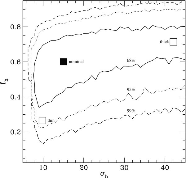
Figure 5. Contour plots of the "minimum significance" statistic for a range of main classical belt models. Each model has a different fraction (fh) of the classical belt in the hot populations with varying choices for the width (σh) of the hot-component. The contours show the locations where the CDF of one of the underlying orbital element distributions have -X- likelihood of being drawn from the model. Contour levels for 68%, 95% and 99% confidence intervals are shown. The best fit model is that which has one dimensional orbital element CDFs that are most likely to have been drawn from the model.
Download figure:
Standard image High-resolution imageAn examination of Figure 5 reveals that our current sample only weakly constrains the width of the main-belt's hot component. This poor constraint is a reflection of the small number of large-inclination objects in our current sample, along with the fact that a given discovery cannot be uniquely assigned to either of these two overlapping components.
If our "thick" model of Figure 5 applies, then based on our survey simulator analysis, all objects in our L3+Pre sample with i < 10° are more likely to be cold-component objects (in the large-i tail of that population) than hot-component members. Thus, in a thick hot-component model, our current sample likely contains only two objects from the hot population and these two TNOs provide only a weak constraint on the hot component's width. If one were to (unjustifiably) assign all the i>7° TNOs to the hot population, the thick model can be rejected at >99% confidence. Thus, although external evidence (from other surveys) suggests that σh ≃ 15°, our current sample provides only a loose confirmation of this result.
In our modeling we have not explored the relation between the hot main classical Kuiper Belt and detached component of the belt which has e>0.24 and a>50 AU. Our current statistics on the distant belt are very limited, however the a>50 AU detached component of the Kuiper Belt may actually be the extension of the hot main classical belt.
5.1.5. Population Estimates
Following the procedure described in Section 4.3, and using the best fit parameters described in the proceeding sections, we compute a population estimate for the main classical belt, giving (see Table 5):
where the uncertainties reflect a 95% confidence limit assuming the underlying orbital model and its parameter values are correct. This population estimate is model dependent, and varies strongly with the width σh of the hot-component. As seen in Figure 5, increasing σh requires a larger fraction of hot-component objects, which increases the population needed to match the observations. This is due to the detection bias against finding hot objects in an ecliptic survey. As a comparison, Table 7 gives the population estimates derived from two other models within the 95% contour. For a "thin disk" model we take the the parameters that minimize the fractional size of the hot population, σh = 10° and fh = 0.2, which produces a population estimate, for the hot-component, that is slightly more than half our best-fit model estimate. For a "thick disk" model we take the acceptable model with fh ∼ 0.7 which gives a population estimate 2-sigma larger than the estimate based on our best-fit parameters. In all three cases the inclination distribution of the cold-component is held constant at σc = 2 2 and we note that the total cold population (which is (1 − fh) × N(Hg < 10)) ranges between 50,000–60,000 for these models. Unsurprisingly the total size of the better-sampled cold population is relatively well determined (∼10%), while the poorly sampled hot-component contains most of the uncertainty (factors of several).
Table 7. Model Dependent Population Estimates
| N(Hg < 10) (1000 s) | Lower | Upper | |
|---|---|---|---|
| Inner Classical Belt | |||
| Two-component P(i) | 2 | 0.3 | 7 |
| One-component P(i) | 8 | 1 | 27 |
| Main Classical Belt (σh, fh) | |||
| (10,0.2) | 74 | 48 | 105 |
| (15,0.6) | 126 | 80 | 177 |
| (40,0.7) | 183 | 112 | 258 |
| Plutinos | |||
| Nominal model | 25 | 13 | 50 |
| Kozai sub-pop | 30 | 15 | 55 |
| α = 0.54 | 12 | 6 | 23 |
Notes. Estimates are given for our model for each subpopulation within the Kuiper Belt. The values in the upper and lower columns are the upper and lower bounds on our 2-σ confidence region for the model-dependent population estimate. All values are in thousands of objects. The Kozai subpopulation shows how forcing half of all plutinos with i>15° to librate in the Kozai resonance causes a small increase in the population estimate.
Download table as: ASCIITypeset image
Figure 6 shows a representation of our underlying model relative to the real L3+Pre detections and a set of simulated detections. In the classical belt's a = 45–47 AU region the survey simulator produces few detections and those that do occur have large eccentricities due to the perihelion flux bias (see also Jones et al. 2006).

Figure 6. Semimajor axis (a) vs. eccentricity (e) and inclination (i) for the main classical belt objects. Filled squares represent the CFEPS L3+Pre sample, the dotted points represent the intrinsic population of the main classical belt, taken from our nominal model.
Download figure:
Standard image High-resolution image5.2. The Plutinos (3:2 Resonant Objects)
There are eight plutinos in the L3+Pre sample. The plutino population is of historical importance as the first recognized resonant subpopulation of the Kuiper Belt (Tholen et al. 1994), and is by far the most numerous in the flux-limited observational catalogs. Plutinos are forced by their resonant argument (e.g., Malhotra 1995, 1996) to come to perihelion away from Neptune (precisely ±90° for a zero libration-amplitude plutino).
Compared to the non-resonant objects, modeling the plutino population is complicated by the need to respect the longitude relations embodied in the resonant argument. For objects in 3:2 mean motion resonance with Neptune the resonant angle ϕ32 has the form:

where λ and ϖ are the object's mean longitude and longitude of perihelion and λN is Neptune's mean longitude.
Plutinos librating in the resonance will have their resonant angle ϕ32 librate around 180° with some amplitude L32. For example, Pluto's resonant angle has a libration amplitude of L32 ≃ 84° (Milani et al. 1989). At maximum libration, the angle between the pericenter direction of Pluto (i.e., λ = ϖ) and Neptune is (180° − 84°)/2 = 48° or (180° + 84°)/2 = 132°; at these extrema the librating relative perihelion longitude reverses direction. This inability to approach Neptune causes the "hole" seen in the on-ecliptic projection of Figure 7.

Figure 7. A planer view of the L3+Pre tracked plutino sample, discovery field location and intrinsic plutino population. The gray area represent the intrinsic Kuiper Belt population produced by our nominal model for the plutino population. The circles are at the discovery locations of our L3+Pre plutinos. For each L3+Pre field we present a box that encloses the approximate boundaries of the region of the solar system that survey was sensitive to. The inner boundary (20 AU) is set by the rate cut in our detection pipeline while the outer limit is set by our flux limit and is drawn at the distance exterior to which we are no longer sensitive to objects with Hg>7.5(Dp ≲ 200 km).
Download figure:
Standard image High-resolution imageThe resonant argument, ϕ32, oscillates sinusoidally around 180°, thus passing more time at the two extrema ϕ32 ± L32 than near 180° itself. The observational impact of this effect is that objects with libration amplitudes of L32 have a bias to being found near (180 ± L32)/2 degrees of longitude away from Neptune. Flux bias weights against the discovery of plutinos far from their current pericenter locations, and so when looking at a particular longitude from Neptune one will tend to find more objects for whom the observed longitude relative to Neptune is such that their resonant argument is at the extrema. Indeed, the L3 plutinos have libration amplitudes similar to the longitudes where they were found. In practice plutinos have L32 < 130°, and so no plutino can be at pericenter in fields that are close to the direction (or antidirection) of Neptune, explaining why the Presurvey, L3q and L3y blocks yielded no plutinos (see Table 1 and Figure 7).
Because of the 1/r4 nature of the reflected flux and the strong bias to detection at certain longitudes, correct modeling of the plutino population requires knowledge of the ecliptic longitudes and flux limits of the surveys. The change in distance from perihelion to aphelion for an e≃0.25 plutino (30–50 AU) drops its apparent magnitude by Δm = 2 magnitudes. Because of the slope of the luminosity function, this change in flux causes a drop by a factor of 10αΔm ∼ 30 in the plutino fraction at longitudes where they are preferentially at aphelion. The dependence of the heliocentric distances at detection on the size distribution is illustrated in Figure 8; if the size distribution is flatter a larger fraction of objects above the flux limit are found at larger distance. The median detection distance varies by more than 2 AU if the power law H-magnitude distribution spans the range of values given in the literature. Therefore, one cannot determine the size distribution of the plutinos from surveys that cover a range of solar longitudes unless one knows the ecliptic longitude of the surveys where plutinos were both detected and not detected. Our characterized survey provides this information, but with only 8 plutinos in the L3+Pre sample, we cannot uniquely constrain this large parameter space since the detected r distribution also depends on the e and ϕ32 distributions.
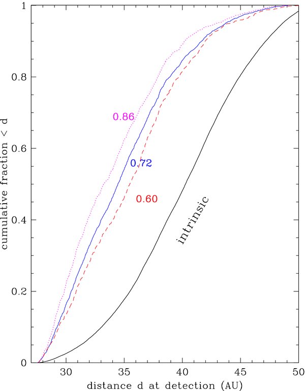
Figure 8. An illustrative example showing the effects of the underlying size distribution on the distance at detection distribution for plutinos. Here we show that the observed distance at detection distribution is steeper for steeper size distributions, even though the intrinsic distance distribution does not change.
Download figure:
Standard image High-resolution imageWe proceeded to find a satisfactory model of the intrinsic plutino orbital element distribution in a two-step process. First we produce hypothetical parametric representations of the intrinsic orbital-element distributions based on available observations and dynamical modeling and then we make small adjustments to these distributions until they are not rejected by the L3+Pre sample.
The a, e limits are taken as the borders of the stable resonance (Morbidelli 1997). A Gaussian e-distribution with mean of 0.21 and standard deviation of 0.06 provides a reasonable match to the observed eccentricity distribution of the plutinos listed in the 3:2 SSBN07 classification (Gladman et al. 2008) and provides an initial model for this element (i.e., we use eccentricity distribution of the MPC reported plutino detections as a proxy for the intrinsic one, with no attempt to correct for detection biases).
Brown (2001) concluded that a single component Gaussian inclination distribution of width 10+3−2 degrees satisfactorily represented that plutino population, so we begin with this 10-degree width.
The libration amplitude, L32, distribution is taken to be a match to the compilation of Lykawka & Mukai (2007); a symmetric "triangle" where the most likely value is 65°, falling to zero at 0° and 130°. The resonant angle ϕ32 cannot be chosen uniformly in the range (180 − L32, 180 + L32) since ϕ32 oscillates sinusoidally in this range; accordingly, we time-weight the ϕ32 oscillation when producing our model distribution of plutinos. Longitudes of node and mean anomalies were chosen randomly. Having picked a resonant angle ϕ32, Equation (6) then forces the value of the plutino's longitude of perihelion ϖ.
This straightforward model produced a/e and distance at detections distributions that are rejected at better than the 99% confidence and an inclination distribution rejected at the 95% confidence level (see Figure 9). To first order the inclination distribution is not strongly coupled to the other distributions, so we proceed by first searching for models that reproduce the observed inclination distribution and then focus on determining the (a, e) and libration amplitude distributions.
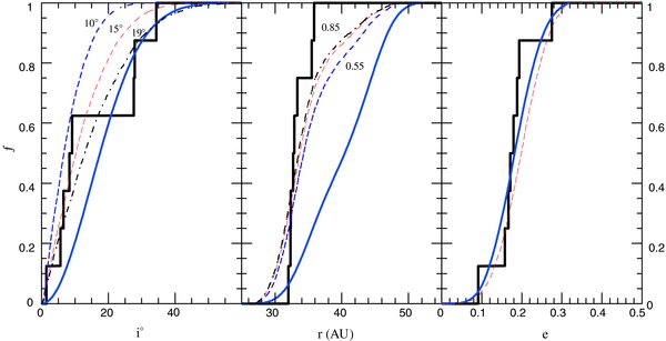
Figure 9. The cumulative distributions of inclination (left panel), distance at detection (center panel), and eccentricity (right panel) for the plutino model. The solid line is the intrinsic population based on the nominal model with a single component Gaussian inclination distribution of width σi = 10° (see text for details of the model). The dashed lines are the simulator-observed distributions based on the various input models. In the left panel the effect of changing the width of the inclination distribution is illustrated, in the center panel the effect of changing the slope of the size distribution is shown, the left panel compares the intrinsic and observed eccentricity distributions. In each panel the histogram is the CDF for the eight L3-Pre plutinos. For the r and e distributions, only models with σi = 15° is shown.
Download figure:
Standard image High-resolution image
5.2.1. The Inclination Distribution of the Plutinos
The CDF of the 8 L3+Pre plutino inclinations is more extended than would be anticipated given a Gaussian of width 10°; the observed population has only a ∼5% chance of being drawn from such an intrinsic distribution. Increasing the intrinsic width of the plutino inclination distribution to 15° provides a more reasonable match, and is intriguingly similar to the width we favor for the hot classical belt. Further widening the inclination distribution to 19° is once again rejected at the 95% confidence level.
That the plutino population appears to have an inclination distribution similar to that of the hot-component of the classical main belt is a cosmogonically intriguing result. The other resonances may also share this inclination distribution but the sample of resonant objects in the L3+Pre sample is not large enough to allow us to explore this possibility.
The three highest-inclination L3+Pre plutinos (of 8) are in fact the three highest-inclination plutinos of the entire MPC "on-ecliptic" catalog. We hypothesize (but cannot prove) a historical bias against the tracking of large-i plutinos discovered in the ecliptic, which may have been initially given larger e (to make SDO orbits) in order to generate the out-of-ecliptic component of their observed motion, resulting in them being lost in subsequent tracking. The lack of high-inclination plutinos in the MPC catalog may thus be partially an artifact of ephemeris bias.
We also examined models where the inclination distribution of the Plutino population matched that of the main classical belt: We find that the Plutino models with the same two component inclination distribution as the main classical Kuiper Belt fail to match the L3+Pre sample and are rejected at more than the 99% confidence level. We conclude that the apparently large fraction of low-i plutinos in the MPC catalog is dominantly due to the bias inherent to looking in the ecliptic.
We caution that a complete model of the plutino populations inclination distribution should take into account the fact that Pluto and some other plutinos are also in the Kozai resonance (Morbidelli 1997), keeping their perihelia (and hence point of maximum detectability) out of the ecliptic plane. This effect generates a very complicated relation between the Kozai fraction and the longitude of the surveys. None of our eight L3+Pre plutinos are librating in the Kozai resonance; in Section 5.2.4 we discuss the impact of this plutino subpopulation on our population estimates.
5.2.2. The a/e and Libration Amplitude Distributions
The reason for our discordance with the straightforward a/e and libration amplitude distribution is simple to understand; detection biases favor discoveries in certain parts of the plutino orbital-element space. In particular, detection of large-e plutinos is heavily favored, resulting in them being over-represented in the MPC catalog. Our survey simulator shows that the "MPC e distribution" would result in ∼40% of our L3+Pre plutinos being detected closer than our closest real detection. We are forced to conclude that the intrinsic plutino e-distribution is more concentrated to lower values. With only eight L3+Pre plutinos, we cannot accurately determine the true eccentricity distribution and have settled on a nominal model of a normal distribution with peak near e = 0.18 and half-width of 0.06.
Another detection bias present in all samples of plutinos is the correlation between observed libration amplitude and the longitude relative to Neptune of the survey field. Thus, although not likely particularly representative of the entire plutino population, we use a libration amplitude distribution modeled after our own detections (most of our plutinos have L32 near 60 or 100 degrees; such objects are favored at the longitudes of our blocks). This model yields an acceptable match (Figure 9) to the L3+Pre detections; that is, we cannot reject the model even if we are also sure that there are detection biases in the angular variables affecting the detected libration amplitudes.
We also examined the result of a flat libration-amplitude distribution (L32 uniform to a maximum value of 130°). This clearly worsened the match and can be rejected at the 99% confidence level. Therefore, the gross characteristic of the detected MPC sample, that the libration amplitudes below 50 degrees and above 110 degrees are depleted (Lykawka & Mukai 2007) appears to be correct, although the functional form of the intrinsic distribution is still poorly constrained.
Inspection of the L3+Pre plutinos yields a puzzle; these eight objects have surprisingly confined distance and eccentricity ranges. We expect that this is a small-numbers statistics problem in this sample and do not have great confidence in our current nominal plutino model. Additional characterized detections will help clarify this question.
Our nominal model of the a/e/i/L32 distribution of the plutions is; a distributed in a way that is consistent with Morbidelli (1997), e following a normal distribution with mean 0.18 and half-width of 0.06, i following a sine-weighted normal with width 15° and a libration amplitude distribution modeled after the values in the L3+Pre sample. This nominal mode for the plutino population, when observed through our survey simulator, provides a statistically acceptable match to the a/e/i distribution of the L3+Pre plutinos.
5.2.3. The Plutino Size Distribution
Both the Hahn & Malhotra (2005) and Elliot et al. (2005) studies suggested the possibility that the plutino size-distribution might be flatter (α = 0.52–0.54) than the rest of the belt. The survey simulator produces poorer matches in the detected distance distribution if we use these lower values of α (i.e., a flatter slope for the plutino size distribution) (see middle panel of Figure 9). Essentially a flat slope implies an increased fraction of large plutinos would be detected at greater heliocentric distances. Thus the distance distribution would have a larger fraction of r>40 AU detections. With only eight L3+Pre plutinos, the survey simulator does not formally reject such a flat H-slope, but such shallow size distributions are found to be less likely and we thus choose to use the same size distribution for the plutino sample as has been determined for the main classical Kuiper Belt, α = 0.72.
5.2.4. Population Estimate
Our nominal model yields an estimated plutino population

(95% confidence, model dependent) as the total plutino population (Table 7).
With only eight detected plutinos, our population estimates are only good to about a factor of two due to the large parameter space which affects detectability. For example, although none of our eight L3 plutinos librate in the Kozai resonance, other high-inclination plutinos do (Lykawka & Mukai 2007). If we assume half of the plutinos with i>15° have their arguments of pericenter librate around 90 or 270 degrees with a width of 50 degrees, then we can increase the estimated population of plutinos to ∼30 000 (Table 7) without violating the lack of a Kozai population in the L3+Pre sample. This occurs because only a few of the L3 blocks probe the longitudes where these plutinos would cross the ecliptic and those that did cross our field of view would not be at pericenter and thus harder to detect. This further reinforces the need for knowledge of the survey longitudes in order to estimate the size of resonant populations.
Changing the nominal model by flattening the size distribution to α = 0.54 causes the population estimate to drop substantially to N(Hg < 10)12, 000, since the plutinos are detectable at greater distances.
Given all the model dependencies, we conclude that the plutino population is ∼25, 000 objects with Hg < 10, to a factor of 2. The nominal estimate indicates that the intrinsic plutino fraction is about 20% of the main classical belt, whose estimate is also uncertain to a factor of 2. Since the majority of Kuiper Belt surveys have been conducted near the ecliptic plane, the fact that the plutino population lacks a cold-component results in an apparent plutino fraction (relative to the classical belt) in the MPC catalog being smaller than the intrinsic one, a fact that some readers may find counter intuitive.
The only previous published plutino population estimate, based on analysis of a KBO survey (Trujillo et al. 2001) is N(Dp>100) = 1400, accurate to a factor of two. Converting our estimate to the same size limit assuming albedo of 0.04 yields an estimate of 9,000, also to a factor of two precision (neglecting the albedo uncertainty). Clearly we estimate a significantly larger plutino population; this is result is due to the fact that the plutino "bias corrections" applied previously assumed the same inclination distribution for the plutinos as for the classical belt. Lacking a cold-component the plutino population is relatively less detectable than the classical belt. We estimate that the plutino population is 40%–50% as numerous as the cold classical main belt population.
The large fraction of plutinos, compared to the main classical belt seems to indicate that Neptune did, at some point, have a slow migration phase which allowed the 3:2 resonance to sweep up a substantial population, although quantitative estimates of the ratio of plutinos to classical objects is lacking except in Hahn & Malhotra (2005). The lack of a low-inclination component in the plutino population, however, appears to be a critical problem for the concept of slow migration into a cold disk.
5.3. The Inner Classical Belt
The inner classical belt is defined as the non-resonant, non-scattering orbits with semimajor axes between Neptune and the 3:2 resonance (Gladman et al. 2008). Duncan et al. (1995) first showed, via long-term numerical simulation, that interior to the a = 39.4 AU semimajor axis of the 3:2, there is a region of orbital stability (from a≃ 36–39 at low e), and remarked with surprise that no objects were known in that region. Petit & Gladman (2003) suggested that the lack of such objects could be due to systematic follow-up bias in early surveys, and showed a handful of such objects derived from more systematic tracking campaigns. Kavelaars et al. (2008) and Parker et al. (2007) discuss this tracking bias in more detail.
Based on current observations and numerical-stability simulations the number of inner classical belt objects is anticipated to be low since the volume of phase space available is much smaller than for the main classical belt. In Gladman et al. (2008), 16 of the 510 TNOs (3%) are classified as inner classical belt objects, which is in rough agreement with our having two such discoveries in the 63-object L3+Pre catalog (L3w06 and L3y14PD). With only two characterized detections we currently provide only a rough population estimate based on a simple phase-space model and must leave exploring the internal orbital structure of this region for the future.
Guided by the results of Duncan et al. (1995) and unpublished integrations by one of the authors (B. Gladman), we have modeled the inner classical belt with the following algorithm. The a/q elements are uniformly distributed in the region a = 37–39 AU and q>35.3 AU. We choose orbital inclinations uniformly from the same double-Gaussian inclination model as for our nominal classical main belt model, σc = 22, σh = 15°, and fh = 0.6 (see Section 5.1), except that we exclude the region 7° < i < 22° in order to account for the strong destabilizing presence of the ν8 secular resonance which passes through the inner classical belt at these inclinations (Knezevic et al. 1991; Duncan et al. 1995). The angles ω, Ω, and M are uniformly distributed between (0,360) degrees.
The number of inner classical belt objects is estimated, subject to our model constraints, using the procedure described in Section 4.3. We find the inner classical belt population to be (see Table 7)
The uncertainty range is the 95% confidence region and is model dependent. The large range of uncertainty is due to the presence of only two detections in the L3+Pre sample. Our two L3+Pre inner-belt detections both have low (i < 5°) inclinations. For the two component i-distribution given above, the "hole" caused by the ν8 resonance results in a very low fraction of detected hot-component inner classical belt TNOs in an ecliptic survey. We calculate that if there is a cold-component then the cold inner-belters should make up ∼96% of the inner-belt CFEPS detections. If, however, the inner belt has only a hot population then low-i (i < 5°) KBOs still represent ∼70% of the expected detections. Under the assumption of a hot only model, (i.e., fh = 1) the size of the intrinsic population required to match the L3+Pre sample would quadruple (Table 7) due to the lower detectability of the intrinsic population. Our 2 low-inclination detections are, of course, consistent with either of these hypothesis.
If we use the CFEPS L3+Pre survey simulations as a proxy for generic KBO surveys conducted near the ecliptic then we might expect the MPC fraction of low and high inclination inner-belt objects discovered near the ecliptic would match that of the simulator. This simulator by proxy appraoch is not too risky, since the non-resonant objects obey no phase relationship with Neptune. Of the 11 inner classical belt objects in the MPC database (Gladman et al. 2008) that were discovered within 2° of the ecliptic, 7 have inclinations of less than 5°. This 64% ratio is close to that expected for an inner-belt containing no cold-component (70%) and in (mild) conflict with the two component model (90%), leading us to suggest that the inner classical belt consists of a purely hot inclination population.
We are cautious not to draw too strong a conclusion from this examination of the MPC database since we expect that inner-belt objects with small inclinations may have been mistakenly classified as plutinos and lost, biasing the MPC against low-i inner-belters. Even with these uncertainties, the inner-belt population is unlikely to exceed 2% of the classical belt population, and may well be smaller than 1%. Reproducing the size and inclination structure of this population will be an important constraint on outer solar system formation models.
6. DISCUSSION
The L3+Pre sample provides a number of new insights into the orbital structures of the Kuiper Belt. We have presented in the preceding sections some quantifiable measure of that orbital structure. In what follows we provide a general interpretation of our observations in light of the current literature on Kuiper Belt formation.
6.1. The Outer Edge of the Main Classical Belt
Based on the L3 sample we have determined that the cold- and hot-components of the main classical belt have distinct eccentricity and semimajor axis distributions. Our modeling of the orbit distribution indicates that the cold main classical belt is isolated in semimajor axis and likely does not extend the full distance to the 2:1 resonance; the cold belt appears to end at ∼46 AU.
Migration models (see Hahn & Malhotra 2005; Chiang et al. 2003; Gomes et al. 2004, for example) produce outer edges to the cold and hot populations by using an initially truncated disk (usually with a pre-migration edge well interior to the current 47.4 AU location of the 2:1 resonance). Many of these models have sought primarily to generate an outer edge at a = 47.4 AU. The fact that we have found different edges (in semimajor axis space, which makes for a fuzzy edge in heliocentric distance) for the hot and cold populations is a new constraint for formation models.
In some outer solar system formation model the radial extent of the cold disk arises as a consequence of the time-scale for the damping of Neptune's eccentricity (see Levison et al. 2008, for example) while the extent of Neptune's migration is controlled by initial radial extent of the planetesimal belt of the solar system (Gomes et al. 2004). Alternatively, the cold classical main Kuiper Belt could be the in situ remains of the primordial solar system and the extent of this population may be indicating the edge of primordial disk. Regardless, formation scenarios are now left to the challenge of producing a cold core whose eccentricity and semimajor axis distributions are distinct from the hot population.
6.2. The Primordial Kuiper Belt
The separate eccentricity and semimajor axis distribution of the hot and cold main classical belt populations add to the growing number of compelling observational differences: different colors (Tegler & Romanishin 1998), different binary fractions (Stephens & Noll 2006), different albedos (Grundy et al. 2005), and perhaps different size distributions (Bernstein et al. 2004; Elliot et al. 2005). Together these imply that the two populations had separate formation locations or processes. Based on the dynamics of the cold-component we feel it likely that this population formed in situ and are more comfortable with models that transfer the hot-component from some other region of the solar system.
The hot main classical belt population has an eccentricity distribution considerably hotter than that of the cold-component, with a semimajor axes distribution that does not exhibit the restriction of the cold-component. Intriguingly, we believe it plausible that the hot-component has the same inclination distribution in the inner classical belt, main classical belt, plutino population, and perhaps other populations not modeled here due to lack of detections.
The hot main classical belt distribution is, in our opinion, compellingly like the high-inclination population produced in Levison et al. (2008) and also somewhat similar to that of Hahn & Malhotra (2005). Testing these models quantitatively will require passing the results of the model simulations through the CFEPS simulator and comparing the resulting orbital distributions to the CFEPS L3+Pre detections. To facilitate quantitative comparison of models with the CFEPS results, the authors provide full details of the survey simulator on the CFEPS Web site (http://www.cfeps.net).
Examining the distribution of MPC inner belters lends evidence to our suggestion that the inner belt lacks a low-inclination component. The authors are not aware of any outer solar system model that predicts a change in the inclination distribution between the inner and main classical belts. Additional evidence for the hot-component membership of the inner belt could come from a census of the colors of the members of this population.
Models of resonance capture during a smooth Neptune migration (Malhotra 1993) indicate that if the large eccentricities of current plutinos are the result of "eccentricity pumping" during resonance migration, the 3:2 resonance must have swept through the inner belt. Resonance capture alone, however, does not strongly affect the inclinations of captured objects (Gomes 2003; Hahn & Malhotra 2005). Thus, if the inner belt had a low-inclination component during the putative resonance sweeping, they should have been easily captured and we should find this cold (low-i) population in the current plutino population; it seems not to be there today. Based on this reasoning, we postulate that the inner belt never had a low-inclination component or it was removed prior to the resonance sweeping migration of Neptune.
In the so-called "Nice" model (Levison et al. 2008) the low-inclination component of the main classical belt is produced by resonance overlap and diffusion in the zone between Neptune and the 2:1 resonance. This mechanism may be very effective at creating a low-i component in the inner belt or at least appears to produce an inner belt with the same inclination distribution as the main classical belt (see Figures 6, 9, and 10 in Levison et al. 2008). More detailed modeling of this scenario and additional observations are needed before a conclusion can be drawn regarding the structure of the inner belt region predicted.
6.3. Plutinos and the Jupiter Family Comets
Is our estimated plutino population large enough to be the source of the Jupiter-family comets (JFCs)? Levison & Duncan (1997) examined the JFC supply problem from the Kuiper Belt as a whole and Morbidelli (1997) quantitatively explored the hypothesis of the gradual gravitational erosion of the plutino population as a supply source for the JFCs and estimated that there would need to be ∼4.5 × 10⁸ objects currently in the 3:2 resonance for this population to be a major source of JFCs.
Our estimate of the plutino population, N(Hg < 10) ∼ 3 × 10⁴, must be scaled by the size-distribution relation to compare with the estimate from Morbidelli (1997). We take, as a plausible estimate, the size of a typical JFC to be D ∼ 5 km (Fernández et al. 1999). Using Equation (4) with an albedo of  gives Hg ∼ 15.7 for a typical, D ∼ 5 km, JFC resulting in ΔHg = 5.7 between the JFC size and the size limit of our population estimate; assuming a uniform power law for the plutino luminosity function with α = 0.72 implies an intrinsic population of N(d>5 km) 4 × 10⁸ plutinos, resulting in the plutinos being a plausible source for the JFC population.
Due to ambiguities in the size distribution slope, the location at which the steep size slope for large objects rolls over to a shallower slope (Bernstein et al. 2004; Petit et al. 2006; Fraser et al. 2008) and the true size of a typical JFC, these numbers should be treated with caution. For example, if JFCs are 10 km rather than 5 km, the corresponding 3:2 population of 3 × 10⁷ objects is insufficient as a supply source.
The sensitivity of these numbers to the unknown value of the typical JFC size is especially worrying, and results in little confidence in a conclusion either for or against a resonant source; we remark that if a resonant source were thought plausible, the now-realized abundant population of objects in high-order resonances beyond the 3:2 (Hahn & Malhotra 2005; Gladman et al. 2008; Lykawka & Mukai 2007) must be seriously examined as an additional source of gradually-destabilized objects which might rival or exceed the 3:2 alone. Arguments favoring the scattering disk as the most likely source of the JFCs (Duncan & Levison 1997) continue to be appealing. Lastly, if either the size distribution of plutinos is shallower, α ∼ 0.52 (Elliot et al. 2005; Hahn & Malhotra 2005) or if the size distribution rolls over to some flat slope as expected then the number of small plutinos drops by a factor of 10 and there are many orders of magnitude too few plutinos available to act as the source of JFCs.
7. CONCLUSIONS
Based on modeling the L3+Pre sample with the CFEPS survey simulator, we conclude:
- 1.The inner classical belt is roughly ∼2%–5% of the population of the main classical belt. The inner classical belt is most likely devoid of a cold-component, but further observations and modeling are needed before the absence of a cold-component can be established.
- 2.The cold classical main Kuiper Belt is a low-i, low-e component tucked into the 42.5 < a < 46 AU zone. The cold-component represents about 40% of the classical main Kuiper Belt population. Models where the semimajor axis distribution of cold-belters is uniform and extends beyond 46.2 AU are rejected at the 95% confidence level. The eccentricities distribution of this component appears to be weighted towards lower values.
- 3.The hot classical main Kuiper Belt contains a population of objects weighted towards large e (P(e) ∝ e) and drawn from a broad inclination distribution well-represented by a Gaussian of width σh ∼ 15°. In fact, this hot belt appears to uniformly fill the stable orbital phase-space between 35 and 47 AU and the detached objects may be the smooth extension of this population to larger a. Current CFEPS observations do not place strong limits on the semimajor axis range of the hot-component of the belt. The hot population represents about 60% of the classical main Kuiper Belt (nonresonant, nonscattering objects between the 3:2 and 2:1 Neptune resonances).
- 4.The 3:2 resonators appear to have an inclination distribution that matches the hot main classical belt and an eccentricity distribution centered around e ∼ 0.2, consistent with stability estimates (Wan & Huang 2001). This population appears to be ∼15% the size of the main classical belt population, although this estimate is highly model dependent.
We have demonstrated the strength of utilizing the CFEPS Survey Simulator to interpret models of the Kuiper Belt's underlying populations. Future Kuiper Belt surveys that provide the detection and tracking details to feed into such a simulator will provide greatly enhanced constraints on the detailed structure of this region of the solar system. We anticipate that the L4 and L5 CFEPS sample will be fully tracked by late-2009, roughly tripling the current L3+Pre sample.
This research was supported by funding from the Natural Sciences and Engineering Research Council of Canada, the Canadian Foundation for Innovation, the National Research Council of Canada, NASA Planetary Astronomy Program NNG04GI29G. This project could not have been a success without the dedicated staff of the Canada-France-Hawaii telescope as well as the assistance of the skilled telescope operators at KPNO and Mount Palomar.
Facilities: CFHT (MegaPrime) CADC KPNO Palomar CTIO WHT
Footnotes
- *
Based on observations obtained with MegaPrime/MegaCam, a joint project of CFHT and CEA/DAPNIA, at the Canada–France–Hawaii Telescope (CFHT) which is operated by the National Research Council (NRC) of Canada, the Institute National des Sciences de l'Universe of the Centre National de la Recherche Scientifique (CNRS) of France, and the University of Hawaii. This work is based in part on data products produced at the Canadian Astronomy Data Centre as part of the Canada–France–Hawaii Telescope Legacy Survey, a collaborative project of NRC and CNRS.
- 11
- 12
Bootstrapping a statistic refers to deriving the value distribution for that statistic via subsampling off a large parent population. In the case discussed here, we create a large parent population via the survey simulator and then draw subsamples of the same size as our observed sample; we then compute the AD or KKS statistics, comparing each subsample's one dimensional orbital-element distributions to that of the simulator produced parent population; finally we determine the fraction of case where our simulated samples, have an AD or KKS statistic larger than the one computed when comparing our observed sample to the large simulator produced parent population.
- 13
Jones et al. (2006) did not provide an inclination distribution for their simple model, here we adopt an Gaussian inclination distribution with a width 15°.