

Abstract
Kernel phase imaging (KPI) enables the direct detection of substellar companions and circumstellar dust close to and below the classical (Rayleigh) diffraction limit. The high-Strehl full pupil images provided by the James Webb Space Telescope (JWST) are ideal for application of the KPI technique. We present a kernel phase analysis of JWST NIRISS full pupil images taken during the instrument commissioning and compare the performance to closely related NIRISS aperture masking interferometry (AMI) observations. For this purpose, we develop and make publicly available the custom Kpi3Pipeline data reduction pipeline enabling the extraction of kernel phase observables from JWST images. The extracted observables are saved into a new and versatile kernel phase FITS file data exchange format. Furthermore, we present our new and publicly available fouriever toolkit which can be used to search for companions and derive detection limits from KPI, AMI, and long-baseline interferometry observations while accounting for correlated uncertainties in the model fitting process. Among the four KPI targets that were observed during NIRISS instrument commissioning, we discover a low-contrast (∼1:5) close-in (∼1 λ/D) companion candidate around CPD-66 562 and a new high-contrast (∼1:170) detection separated by ∼1.5 λ/D from 2MASS J062802.01-663738.0. The 5σ companion detection limits around the other two targets reach ∼6.5 mag at ∼200 mas and ∼7 mag at ∼400 mas. Comparing these limits to those obtained from the NIRISS AMI commissioning observations, we find that KPI and AMI perform similar in the same amount of observing time. Due to its 5.6 times higher throughput if compared to AMI, KPI is beneficial for observing faint targets and superior to AMI at separations ≳325 mas. At very small separations (≲100 mas) and between ∼250 and 325 mas, AMI slightly outperforms KPI which suffers from increased photon noise from the core and the first Airy ring of the point-spread function.
Export citation and abstract BibTeX RIS

Original content from this work may be used under the terms of the Creative Commons Attribution 3.0 licence. Any further distribution of this work must maintain attribution to the author(s) and the title of the work, journal citation and DOI.
1. Introduction
The recently commissioned James Webb Space Telescope (JWST) is a joint NASA/ESA/CSA flagship science mission to explore the beginnings of the Universe, the assembly of galaxies, the birthplaces of stars, and planetary systems and the origins of life (Gardner et al. 2006). For the direct observation and characterization of giant exoplanets and circumstellar dust, JWST is equipped with multiple coronagraphic imaging modes in the near- and mid-infrared as well as a non-redundant mask (NRM) operating between ∼2.8 and 4.8 μm that transforms the 6.5 m primary mirror into an interferometric array of seven subapertures (Artigau et al. 2014). It is the first time in history that such an aperture mask is available on a space-based telescope. By exploiting the interferometric capabilities of this mask, the NIRISS instrument (Doyon et al. 2012) is expected to enable high-contrast imaging up to ∼10 mag contrast at small angular separations of ∼70–400 mas (Greenbaum et al. 2015), well inside the inner working angle (IWA) of the NIRCam coronagraphs (half width half maximum of ∼6 λ/D, where λ is the observing wavelength and D is the telescope primary mirror diameter, Krist et al. 2009, 2010). The unique parameter space accessible with the NIRISS NRM enables advances in exoplanet and planet formation as well as galaxy evolution science by studying close-in stellar and substellar companions, warm exozodiacal dust around nearby stars, transitional disks, and feedback in active galactic nuclei for instance (Sivaramakrishnan et al. 2023).
While the NIRISS NRM transforms JWST into an interferometer and thereby enables high-contrast imaging down to the Michelson diffraction limit (∼0.5 λ/D), the NRM also blocks ∼85% of the incoming light and thus significantly reduces the sensitivity of the observations (Artigau et al. 2014). An alternative technique that is not affected by such a big throughput loss is called "kernel phase imaging" (KPI) and has been introduced by Martinache (2010). KPI uses Fourier quantities of full pupil images to achieve the same high resolution (∼0.5 λ/D) as aperture masking interferometry (AMI). The basic idea of KPI is to discretize the full pupil into an interferometric array of "virtual" subapertures during post-processing. However, due to the high redundancy of the full pupil, KPI requires high-Strehl images (which are naturally given from space in the absence of a disturbing atmosphere) so that the image Fourier phase can be linearized and the contributions from individual baselines can be disentangled. In this linear regime, the relationship between the image Fourier phase ϕ and the pupil plane phase φ reads

where A is the matrix mapping baselines in the pupil plane to spatial frequencies in the image Fourier plane, R is the diagonal matrix encoding the redundancy of each baseline, and ϕobj is the image Fourier phase intrinsic to the observed object. One can then multiply Equation (1) with R from the left, obtain the kernel K of the baseline mapping matrix A via singular value decomposition, and derive the kernel phase


which is independent of pupil plane phase errors to first order (higher order terms appear because the linearization applied here is only an approximation, Ireland 2013). Therefore, kernel phase has similar properties as closure phase in AMI and Ireland (2016) has shown that kernel phase is a generalization of closure phase to the case of redundant apertures. Hence, KPI with JWST is expected to achieve similar performance as AMI except for an increased sensitivity to faint targets due to its increased throughput.
With NIRISS, KPI can be used with the same four filters as AMI, which are F277W, F380M, F430M, and F480M, albeit the usefulness of F277W is limited given that the NIRISS detector is undersampled at this wavelength. The AMI observing template, which is also used for KPI observations, provides repeatable target acquisition on a predefined detector position to subpixel accuracy (typically <0.1 pixels Rigby et al. 2022). Using the same detector position for the science and the PSF reference target will help mitigating systematic errors (e.g., from flat-fielding). The methods presented here are based on a monochromatic description of the image and given the ∼6% bandwidth of the medium-band filters mentioned above, we expect some level of spectral decoherence for both AMI and KPI techniques. While a detailed study of this effect is beyond the scope of this paper, we note that kernel phase techniques have been successfully applied to Hubble Space Telescope (HST) wide-band (F110W) images by Pope et al. (2013). To minimize calibration errors, we recommend to use a PSF reference target with a similar spectral type as the science target. In the model fitting process with fouriever (Section 2.3), it is possible to apply bandwidth smearing to account for the finite filter bandpass of the observations. Finally, since KPI can be applied to any full pupil image, it can be used with all instruments onboard JWST opening up the entire wavelength range of ∼0.7–25.5 μm for high-resolution imaging. KPI's increased uv-coverage with respect to AMI also enables high-contrast image reconstruction of complex scenes down to the Michelson criterion. For a more detailed description of kernel phase we refer the reader to Martinache (2010) and Martinache et al. (2020).
The first application of KPI can be found in Martinache (2010) who detected a previously known companion to the star GJ 164 at a contrast of ∼9:1 and a separation of ∼0.6 λ/D in archival HST NICMOS data, clearly demonstrating the super-resolution power of KPI. Later, Pope et al. (2013) discovered five new brown dwarf companions with separations ranging from ∼0.4 to 0.6 λ/D, also in archival HST NICMOS data. The first time that KPI was applied behind an adaptive optics system from the ground was in Pope et al. (2016) who observed the known binary α Oph with both KPI and AMI and found excellent agreement between the binary parameters derived from both techniques. Kammerer et al. (2019) and Wallace et al. (2020) went one step further and searched for close-in substellar companions in an archival VLT NACO data set of nearby field stars and a Keck NIRC2 data set of young stars in the Taurus Molecular Cloud where they achieved contrast limits of up to ∼7 mag at ∼1 λ/D in the L-band. Kammerer et al. (2019) and Laugier et al. (2019) came up with different methods to extend the dynamic range of KPI observations beyond the saturation limit in the central few pixels of the core of the point-spread function (PSF). The method from Kammerer et al. (2019) is also implemented in the JWST kernel phase pipeline presented here and explained in more detail in Section 2.1.1. Similar to angular differential imaging (Marois et al. 2006) in classical high-contrast imaging, Laugier et al. (2020) also derived self-calibrating angular differential kernel phase observables, but these are more suitable for data sets with larger field rotation than JWST can provide. To measure the photometry of the individual components of the T Tau triple star system at ∼10 μm, Kammerer et al. (2021) applied KPI to VLT VISIR-NEAR observations in the mid-infrared, demonstrating the feasibility of KPI with instruments such as JWST MIRI. Recently, pioneering work from Pope et al. (2021) has shown that automatic differentiation methods can be used to extract kernel phase observables from any differentiable optical system, such as a Lyot coronagraph for instance, which has previously been impossible given that focal plane masks destroy the linearity of the Fourier phase observables. Albeit beyond the scope of this paper, automatic differentiation methods are a viable alternative beyond the classical KPI methods presented here.
The paper is structured as follows. Section 2 describes the methods that we use to reduce and analyze the JWST NIRISS KPI commissioning data. In particular, Section 2.1 introduces our customly developed and publicly available stage 3 kernel phase data reduction pipeline that can be used to extract kernel phase observables from JWST images in a similar fashion as the other STScI jwst 24 data reduction pipelines. Section 2.2 motivates the need for a dedicated kernel phase data exchange format and describes the KPFITS file format that we are proposing here. Section 2.3 introduces our publicly available model fitting toolkit fouriever that can be used to search for companions or determine detection limits from OIFITS (a widely used file format for exchanging AMI and long-baseline interferometry data, Pauls et al. 2005; Duvert et al. 2017) and KPFITS files. The NIRISS KPI commissioning observations are described in Section 3 and our results from their analysis are presented and discussed in the context of the NIRISS AMI commissioning observations in Section 4. Finally, Section 5 summarizes our work and draws conclusions for the application of AMI and KPI with JWST.
2. Methods
For reducing and analyzing the JWST NIRISS KPI commissioning data, we develop a variety of custom and user-friendly software that we make publicly available on GitHub. This enables other JWST observers to use our tools for proposal planning and for getting science-ready data products and plots out of their own programs.
2.1. Kernel Phase Stage 3 Pipeline
The STScI jwstdata reduction pipeline is organized into three stages. Stage 1 performs detector level calibrations such as bias correction and jump detection, stage 2 performs photometric calibrations, and stage 3 performs high-level calibrations that are specific to each of the observing modes supported by JWST (e.g., AMI, coronagraphic imaging, integral field spectroscopy). To enable the community a straightforward access to kernel phase observables from JWST images, we develop a custom stage 3 pipeline that we name the Kpi3Pipeline. 25 This pipeline can be used for extracting kernel phase observables from full pupil NIRISS and NIRCam images, support for MIRI will be added in a future update. Before the JWST images can be fed into the Kpi3Pipeline, they need to be processed with the jwststage 1 and 2 pipelines. For those, similar as with AMI data, we recommend to skip the inter-pixel capacitance, the photometry, and the resample step since Fourier plane imaging techniques in general are highly sensitive to variations in the pixel-by-pixel response of the detector (e.g., Ireland 2013). Skipping these steps avoids systematic errors being introduced by the pipeline corrections. Instead, the approach with NIRISS KPI and AMI observations is to center the science and the reference targets on the exact same detector pixel and thereby minimize flat-fielding errors. The available detector positions were carefully chosen to provide both a good uv-coverage of the pupil support (which is challenging with NIRISS given its coarse sampling) and a clean detector region with only few bad pixels (Sivaramakrishnan et al. 2023). Dithering is hence not recommended for NIRISS KPI (and AMI) observations. While the backend of the Kpi3Pipelineis based on XARA 26 (Martinache 2010, 2013; Martinache et al. 2020), the front end is designed similarly to the STScI jwstpipelines to provide a uniform experience for the user. Similar to the VLT NACO kernel phase data reduction pipeline developed by Kammerer et al. (2019), the Kpi3Pipelineconsists of five steps:
- 1.bad pixel fixing step,
- 2.recentering step,
- 3.windowing step,
- 4.kernel phase extraction step,
- 5.empirical uncertainties step.
An intermediate data product can be saved after each step so that the individual steps can be run separately and each of the five steps can generate a diagnostic plot for validation purposes. Each step and its diagnostic plot is described in more detail below. A list of the tunable parameters of each step can be found in Appendix B (Table 4). In principle, all steps except for the fourth one can be skipped although it is highly recommended to run at least steps 1, 2, and 4 to ensure that the kernel phase extraction step is provided with properly preprocessed data.
An additional input that is required for running the Kpi3Pipeline is a discrete model of the pupil. We note that due to different pupil plane masks, the NIRISS, NIRCam, and MIRI instruments all see slightly different pupils. We provide default pupil models for the NIRISS CLEARP and the NIRCam CLEAR pupils but the user can also provide a custom pupil model if desired. For the default pupil models, we distribute subapertures on a hexagonal grid so that 19 subapertures fall inside one JWST primary mirror segment. To obtain an isotropic grid, we also distribute subapertures on top of the gaps between the individual primary mirror segments. We are using a "gray" pupil model so that the subapertures on top of the gaps have a slightly reduced transmission. Then, we apply the transmission of the instrument-specific pupil mask and discard all subapertures with a total transmission of <0.7. This results in the NIRISS CLEARP pupil model shown in Figure 1. This model consists of 349 individual subapertures spanning 948 distinct baselines. After discarding all baselines with a redundancy of less than 10, 800 distinct baselines yielding 452 individual kernel phases remain. Discarding baselines with low redundancy helps to avoid the longest (and most noisy) baselines at the edge of the primary mirror. We find that a redundancy threshold of 10 is sufficient to avoid Fourier phases >0.5 rad and entering the non-linear regime.

Figure 1. Left: NIRISS CLEARP pupil mask used for full pupil imaging. The total throughput of the mask is ∼84%. Right: pupil model used for the kernel phase analysis of the NIRISS commissioning data. The model consists of 349 individual subapertures spanning 948 distinct baselines. Each subaperture has a transmission 0.7 < T ≤ 1 that was determined by averaging the NIRISS CLEARP pupil mask transmission over the hexagonal grid shown in gray. Subapertures with a total transmission of <0.7 were discarded.
Download figure:
Standard image High-resolution image2.1.1. Bad Pixel Fixing Step
Bad pixels can have a ruinous impact on Fourier plane imaging since an individual bad pixel contributes noise to all spatial frequencies of the image. However, Ireland (2013) has shown that bad pixels do not affect kernel phase observables if they are properly corrected. In the Kpi3Pipeline, bad pixels can be fixed using two different methods: "medfilt" or "fourier". In both cases, the locations of the bad pixels are obtained from the jwst stage 1 pipeline. As a default, all pixels flagged as "DO_NOT_USE" in the data quality array are considered as bad pixels but the user may specify other data quality flags
27
that shall be considered as bad pixels. With the "medfilt" method, bad pixels are simply replaced with the median filtered image using a kernel size of five pixels. With the "fourier" method, bad pixels are fixed by minimizing their Fourier power outside the region of support permitted by the pupil geometry. This method was introduced by Ireland (2013) and starts by computing the matrix
B
Z
which maps the bad pixel values x onto the Fourier domain Z (the complement of the pupil support), so that their Fourier power  is given by

where b are the corrections to be made to the bad pixels and  Z
is remaining noise. These corrections are obtained by computing the Moore-Penrose pseudo inverse of
B
Z
and solving for
Z
is remaining noise. These corrections are obtained by computing the Moore-Penrose pseudo inverse of
B
Z
and solving for

where the star denotes the complex conjugate. This algorithm has been successfully applied to fix bad and reconstruct saturated pixels in kernel phase observations by Kammerer et al. (2019) and is described in more detail in Sivaramakrishnan et al. (2023). While the "fourier" method is particularly suited for reconstructing saturated PSFs, we do not have any saturated PSFs in the NIRISS KPI commissioning data and therefore use the "medfilt" method for simplicity. The diagnostic plot of the bad pixel fixing step is shown in Figure 2.

Figure 2. Diagnostic plot produced by the bad pixel fixing step of the Kpi3Pipeline for the first frame of TYC 8906-1660-1 observed with JWST NIRISS full pupil imaging. The left panel shows the bad pixel map from the jwst stage 1 pipeline considering the specified data quality flags as bad pixels (here DO_NOT_USE), the middle panel shows the frame in a logarithmic color stretch before fixing the bad pixels, and the right panel shows it after fixing the bad pixels using the "medfilt" method. The bottom five rows are reference pixels for correcting bias drifts which are not used for science.
Download figure:
Standard image High-resolution image2.1.2. Recentering Step
As mentioned in Section 1, the image Fourier phase needs to be in the linear regime in order for the kernel phase technique to be applicable. Hence, recentering the images is important since a PSF being offset from the image center by only half of a pixel would already result in a linear ramp in the image Fourier phase from −π/2 to +π/2 across the support of the telescope pupil (i.e., the modulation transfer function of the pupil). While the kernel phase observables are independent of first order pupil plane phase errors (and thus a linear ramp in the image Fourier phase, Martinache 2010), there are virtually always systematic phase errors that can easily cause the image Fourier phase wrapping around the ±π discontinuity if added on top of a linear phase ramp and thereby destroying the properties of the kernel phase observables. To avoid this, the Kpi3Pipeline uses the Fourier phase norm minimization (FPNM) method implemented in XARA that recenters the images using a least-squares gradient descent minimization of the norm of the image Fourier phase within the support of the telescope pupil. This method was shown to be more robust, especially in the presence of low-contrast companions at small angular separation (Kammerer et al. 2019), albeit slightly slower than the other two methods (BCEN = centroid of the brightest speckle & COGI = center of gravity of the image) that are also implemented in XARA. We note that before recentering the images, we trim them to their maximum possible square size (constrained by the location of the detector edges) around the expected PSF center (the reference pixel position where JWST aims to place the PSF during target acquisition 28 ). The diagnostic plot of the recentering step is shown in Figure 3.

Figure 3. Diagnostic plot produced by the recentering step of the Kpi3Pipeline for the same data as shown in Figure 2. The left panels show the full frame (top) and a zoom on the PSF (bottom) before recentering and the right panels show them after recentering. The red crosshair indicates the identified PSF center.
Download figure:
Standard image High-resolution image2.1.3. Windowing Step
Windowing with a smooth function is an effective method to mitigate artifacts when numerically Fourier transforming images with sharp edges. Since XARA uses a Fourier transform to extract kernel phase observables from the telescope images, we window (i.e., multiply) them with a super-Gaussian windowing function w of shape

before Fourier transforming them, where x and y are the pixel coordinates with respect to the image center and r is the radius of the super-Gaussian windowing function in units of pixels. The radius r is chosen adaptively as the smaller of 40 pixels and a fourth of the trimmed square image size to make sure that the window is not larger than the image itself. If the images are large enough, a radius of 40 pixels gives access to separations of at least 5 λ/D (sometimes more depending on the observing wavelength). At these separations, classical high-contrast imaging techniques such as coronagraphy are typically superior to KPI. The NIRISS full pupil images considered for the KPI analysis here do only have a native size of 80 by 80 pixels and we are using a constant window radius of r = 15 pixels for them resulting in a field-of-view of ∼2'', which is more than sufficient for the region where NIRISS KPI is superior to NIRCam coronagraphy (Kammerer et al. 2022). The diagnostic plot of the windowing step is shown in Figure 4.

Figure 4. Diagnostic plot produced by the windowing step of the Kpi3Pipeline for the same data as shown in Figure 2. The left panel shows the trimmed and recentered image before windowing and the right panel shows it after windowing with a super-Gaussian windowing function with a radius of 20 pixels. For reference, the dashed red circle indicates a radius of 20 pixels from the center.
Download figure:
Standard image High-resolution image2.1.4. Kernel Phase Extraction Step
Once the bad pixels are fixed and the images are recentered and windowed, kernel phase observables can be extracted using XARA. First, the image Fourier phase ϕ at the discrete spatial frequencies of the pupil model is obtained using a linear discrete Fourier transform. Then, the kernel phase θ is computed as

where  and
K
is the kernel of the pupil model
A
as described in Martinache (2010). We also decided to normalize the rows of the
and
K
is the kernel of the pupil model
A
as described in Martinache (2010). We also decided to normalize the rows of the  matrix to one so that the amplitude of the kernel phase signal is no longer depending on the geometry of the pupil model. This enables a more direct comparison between kernel phase observables obtained from different telescopes/instruments. To analytically estimate the kernel phase uncertainties, we first need to linearize the relationship between the kernel phase θ and the image I, so that

where F denotes the linear discrete Fourier transform at the spatial frequencies of the pupil model and the fraction denotes element-wise division (Kammerer et al. 2019). Then, the kernel phase covariance Σ can be computed from the image covariance Σimage as

where Σimage is assumed to be uncorrelated with the square of the "ERR" extension of the stage 2-reduced pipeline product on the diagonal.
If the recentering step is being run in conjunction with the kernel phase extraction step, a more accurate method is used to extract the kernel phase observables where the integer pixel recentering is performed by rolling the image and the subpixel recentering is performed by adding a linear ramp to the extracted image Fourier phase. This method circumvents interpolation errors when performing subpixel shifts of the images. We note that for extracting the kernel phase uncertainties, we still use the images that have been recentered with subpixel precision. The diagnostic plot of the kernel phase extraction step is shown in Figure 5.

Figure 5. Diagnostic plot produced by the kernel phase extraction step of the Kpi3Pipeline for the same data as shown in Figure 2. The upper left panel shows the image Fourier phase together with the discrete spatial frequencies of the pupil model (red dots). The bottom panels show the image Fourier phase extracted at the discrete spatial frequencies of the pupil model (left) and the resulting kernel phase (right). In both panels, the theoretical signal of an unresolved point-source is constantly zero and indicated by a dashed black line. The upper right panel shows the kernel phase correlation matrix obtained from a linear propagation of the image pixel uncertainties (see, Equation (11)).
Download figure:
Standard image High-resolution image2.1.5. Empirical Uncertainties Step
A single JWST data product (here called an exposure) typically consists of a large number (≳10) of individual integrations. While all previous pipeline steps can be performed on hundreds of individual images within timescales of seconds to minutes, it can be very time- and memory-consuming to perform model fitting on such a large number of individual data points, especially if accounting for correlated uncertainties. Hence, it is advisable to average individual integrations within a single exposure into one final data point. This is achieved in the Kpi3Pipeline by computing the covariance-weighted mean of the kernel phase observables according to

where θi and Σi are the kernel phase and its covariance of the individual integrations and

is the mean covariance matrix (Kammerer et al. 2019).
Another advantage of having several individual integrations is that the uncertainties can be estimated empirically as the standard deviation of the kernel phase observables over these individual integrations. This can be especially helpful if the kernel phase observables are dominated by systematic errors (e.g., Kammerer et al. 2019; Wallace et al. 2020) which are not reflected in the analytical error estimation from the previous pipeline step. An empirical estimation for the kernel phase covariance can then be obtained by computing the correlation matrix C mean of Σmean (which only includes image pixel uncertainties) and multiplying it with the empirically estimated kernel phase standard deviation σemp, that is

Here, m and n denote the indices of the matrices. This procedure ensures that the kernel phase uncertainties remain consistent with the square root of the diagonal of the kernel phase covariance matrix. The diagnostic plot of the empirical uncertainties step is shown in Figure 6.

Figure 6. Diagnostic plot produced by the empirical uncertainties step of the Kpi3Pipeline for the same data as shown in Figure 2. The minimum/maximum range over the exposure is shown as a light blue area and the weighted mean including uncertainties is shown as a solid blue line.
Download figure:
Standard image High-resolution image2.2. Kernel Phase FITS Files
A common and well-defined data exchange format has proven highly valuable for sharing astronomical data and reproducing observational results. In the optical and near-infrared (long-baseline) interferometry community, the OIFITS file format (Pauls et al. 2005; Duvert et al. 2017) has established itself as a golden standard that is used by most major observatories and instruments (e.g., CHARA/MIRC, Monnier et al. 2004, VLTI/PIONIER, Le Bouquin et al. 2011, VLTI/GRAVITY, Lapeyrere et al. 2014) and data analysis tools (e.g., LITpro, Tallon-Bosc et al. 2008, CANDID, Gallenne et al. 2015). Due to the very similar nature of the data, the same OIFITS file format is also being used for AMI data (e.g., in ImPlaneIA, Greenbaum et al. 2015, AMICAL, Soulain et al. 2020, SAMpip
29
). Although KPI and AMI are closely related techniques (see, e.g., Ireland 2016), there are a few subtle differences that strongly motivate the need for a distinct file format for KPI data. First, as shown in Section 1, the kernel phase θ is obtained from a special linear combination  of the image Fourier phase ϕ. Thus, the kernel matrix
  is of fundamental importance in KPI and is repeatedly used in the model fitting process to project image Fourier phase onto kernel phase. Fast and easy access to this kernel matrix
  is therefore vital. While it is in principle possible (albeit time-consuming) to recompute this matrix from the geometry of the pupil array that can be saved in the OI_ARRAY extension of an OIFITS file, we strongly prefer to save this matrix directly in one of the FITS file extensions, not least because handling hundreds of individual subapertures becomes impractical using the OI_ARRAY extension. Second, recent work from Martinache et al. (2020) has shown that the use of "gray" pupil models featuring subapertures with a continuous transmission 0 < T ≤ 1 is highly desirable in KPI as they help to reduce the systematic kernel phase signal of unresolved and point-like PSF reference targets. However, gray pupil models are not supported by the OIFITS file format due to the third dimension required to store transmission. Finally, the Karhunen-Loève calibration method applied in Kammerer et al. (2019); Wallace et al. (2020), and Kammerer et al. (2021) can be used implicitly if the kernel phase θ and the kernel matrix
  are saved in matrix format. This is because the Karhunen-Loève calibration (Soummer et al. 2012) is a linear projection represented by a matrix
P
so that replacing the kernel phase and the kernel matrix with
P
· θ and
are saved in matrix format. This is because the Karhunen-Loève calibration (Soummer et al. 2012) is a linear projection represented by a matrix
P
so that replacing the kernel phase and the kernel matrix with
P
· θ and  , respectively, will ensure that any model fitting code will automatically run correctly with a calibrated data set.
Based on the aforementioned issues with the OIFITS file format, the kernel phase community has expressed the need for a dedicated data exchange format in the framework of the Masking/Kernel Phase Hackathon 30 held virtually in mid 2021 to ensure compatibility among a variety of data reduction, calibration, and model fitting tools. The kernel phase FITS (KPFITS) file format proposed here is based on the XARA file format developed by Martinache (2010) and Martinache (2013). However, based on recent developments from Kammerer et al. (2019) and Martinache et al. (2020) several modifications were made to the original XARA file format in consultation with kernel phase experts from the global community. For completeness, we also added an optional extension for saving kernel amplitude observables as introduced in Pope (2016). The structure of the KPFITS file format is described in Table 1 and shall be used as a standard for saving and exchanging kernel phase data in the future. The exact order of the FITS file extensions is in principle irrelevant as extensions shall be referred to in the code with their extension names, the numbering in Table 1 can hence be regarded a suggestion. We note that in principle, AMI data can also be exchanged using the KPFITS file format in a more efficient way.
Table 1. Structure of the KPFITS File Format
| Ind | Opt | Name | Type | Dimensions | Description |
|---|---|---|---|---|---|
| 0 | (N) | PRIMARY | Image | Nf × Nλ × Npix × Npix | Telescope images (can be empty array) |
| 1 | N | APERTURE | Table | Nsap × 3 | Description of pupil model |
| N | XXC | Column | Subaperture x-coordinate [m] | ||
| N | YYC | Column | Subaperture y-coordinate [m] | ||
| N | TRM | Column | Subaperture transmission (0 < T ≤ 1) | ||
| 2 | N | UV-PLANE | Table | Nuv × 3 | Fourier plane coverage of pupil model |
| N | UUC | Column | Fourier u-coordinate [m] | ||
| N | VVC | Column | Fourier v-coordinate [m] | ||
| N | RED | Column | Redundancy of uv-position (integer) | ||
| 3 | N | KER-MAT | Image |

| Matrix  mapping image Fourier phase onto kernel phase mapping image Fourier phase onto kernel phase |
| 4 | N | BLM-MAT | Image | Nuv × Nsap | Matrix A mapping pupil plane phase onto image Fourier phase |
| 5 | N | KP-DATA | Image |

| Kernel phase data [rad] |
| 6 | N | KP-SIGM | Image |

| Kernel phase uncertainties [rad] |
| 7 | N | CWAVEL | Table | Nλ × 2 | Description of bandpass |
| N | CWAVEL | Column | Central wavelength of bandpass [m] | ||
| N | BWIDTH | Column | Best available estimate of effective half-power bandwidth [m] | ||
| 8 | N | DETPA | Image | Nf | Detector position angle E of N [deg] |
| 9 | N | CVIS-DATA | Image | 2 × Nf × Nλ × Nuv | Complex visibility data (dim 1 = real part, dim 2 = imag. part) |
| >9 | Y | KA-DATA | Image |

| Kernel amplitude data |
| >9 | Y | KA-SIGM | Image |

| Kernel amplitude uncertainties |
| >9 | Y | CAL-MAT | Image |

| Karhunen-Loève projection matrix  as in K19 as in K19 |
| >9 | Y | KP-COV | Image | Flexible, up to 
| Kernel phase covariance [rad2] |
| >9 | Y | KA-COV | Image | Flexible, up to 
| Kernel amplitude covariance |
| >9 | Y | FULL-COV | Image | Flexible, up to 
| Kernel phase [rad 2] and kernel amplitude covariance |
| >9 | Y | IMSHIFT | Table | Nf × 2 | Shift to recenter images |
| Y | XSHIFT | Column | Shift along x-axis (1-axis in Python) [pix] | ||
| Y | YSHIFT | Column | Shift along y-axis (0-axis in Python) [pix] | ||
| >9 | Y | WINMASK | Image | Npix × Npix | Super-Gaussian windowing mask |
Note. "Ind" denotes the index of the FITS file extension, "Opt" specifies whether an extension is optional or not, Nf denotes the number of frames, Nλ
denotes the number of spectral channels, Npix denotes the number of pixels per image axis, Nsap denotes the number of subapertures, Nuv denotes the number of uv-points and  denotes the number of kernels. We note that the telescope images are optional and the PRIMARY extension can in principle be an empty array. K19 = Kammerer et al. (2019). All data should be of type float.
Download table as: ASCIITypeset image
To ensure that the information necessary to consistently reprocess the kernel phase data is present, the KPFITS file format also requires a PRIMARY FITS header with the header keywords specified in Table 2. While several of these keywords are optional, others are strictly required to rerun the Kpi3Pipeline and extract kernel phase observables or to aid the model fitting procedures described in Section 2.3.
Table 2. PRIMARY Header of the KPFITS File Format
| Opt | Name | Type | Unit or Value | Description |
|---|---|---|---|---|
| N | PSCALE | float | mas/pix | Detector pixel scale |
| N | GAIN | float | ADU/e- | Detector gain |
| N | DIAM | float | m | Primary mirror diameter |
| N | EXPTIME | float | s | Exposure time per frame |
| N | TELESCOP | str | e.g., JWST | Telescope name |
| N | INSTRUME | str | e.g., NIRISS | Instrument name |
| Y | DATEOBS | str | YYYY-MM-DDTHH:MM:SS | Date of observation |
| Y | TARGNAME | str | e.g., AX Cir | Target name |
| Y | TARG_RA | float | deg | Target RA (mid exposure) |
| Y | TARG_DEC | float | deg | Target DEC (mid exposure) |
| Y | FILTER | str | e.g., F480M | Filter name |
| Y | POLCHANN | str | ⋯ | Polarization channel |
| Y | PATTTYPE | str | e.g., NONE/5-POINT-BOX | Dither pattern name |
| Y | PATT_NUM | int | e.g., 1 | Position number in dither pattern |
| Y | NUMDTHPT | int | e.g., 5 | Total number of positions in dither pattern |
| Y | PROCSOFT | str | e.g., XARA | Processing software name |
| Y | WRAD | float | pix | Radius of super-Gaussian windowing mask |
| Y | CALFLAG | str | True/False | Has the data been calibrated? |
| N | CONTENT | str | KPFITS1 | Name of file format |
Note. "Opt" specifies whether a header keyword is optional or not.
Download table as: ASCIITypeset image
2.3. Model Fitting with fouriever
There are several publicly available model fitting toolkits that understand OIFITS files and can be used to analyze long-baseline interferometry and AMI data (e.g., LITpro, Tallon-Bosc et al. 2008, CANDID, Gallenne et al. 2015, PMOIRED, Mérand 2022). However, none of these toolkits accounts for correlated uncertainties in the fits. Recently, Lachaume et al. (2019) and Kammerer et al. (2020) developed methods to extract and model correlations in long-baseline interferometry data and Kammerer et al. (2020) showed that accounting for them in the fits can improve VLTI/GRAVITY companion detection limits by a factor of up to ∼2. More importantly, they also found that widely used detection criteria based on χ2-statistics are only valid when accounting for correlations and yield an excessive number of false positive detections otherwise.
In light of these findings, we develop the fouriever toolkit which provides a single solution for analyzing KPI, AMI, and long-baseline interferometry data while accounting for correlated uncertainties in the fits. The toolkit also enables modeling correlations in long-baseline interferometry and AMI data as described in Kammerer et al. (2020) and calibrating science data using a Karhunen-Loève projection based on calibrator data as introduced in Kammerer et al. (2019). The fouriever toolkit is written in Python and can be obtained from GitHub. 31 Many functionalities were inspired by CANDID but have been modified to improve the performance given that fits accounting for correlations involve significantly more complex matrix multiplications. In the following, we briefly outline the search for companions and the estimation of detection limits with fouriever and highlight similarities and improvements with respect to CANDID. We also note that fouriever comes with tutorials and test data for JWST NIRISS AMI, VLT NACO and Keck NIRC2 KPI, and VLTI PIONIER and VLTI GRAVITY long-baseline interferometry applications.
2.3.1. Companion Search
The first step in the analysis of high-contrast imaging data usually consists of the search for one or multiple companions. For this purpose, fouriever can compute a χ2-detection map based on binary model fits similar to the fitMap in CANDID but accounting for correlated uncertainties in the fits. This χ2-detection map is obtained from a set of least squares gradient descent minimizations initialized on a grid around the science target. The optimizer aims to minimize

where R = D − M are the residuals between data and model and Σ is the data covariance matrix. For simplicity, other toolkits assume that there are no correlations and that the matrix Σ is diagonal. The model observables are obtained from the complex visibility of a binary source

where V1 and V2 are the complex visibilities of the primary and the secondary, f is the relative flux of the secondary with respect to the primary, ΔRA and ΔDEC are the R.A. and decl. offset between the primary and the secondary, u and v are the Fourier plane coordinates for which the complex visibility shall be obtained, and λ is the observing wavelength (e.g., Berger 2003). For the case of an unresolved companion considered here, we set


where J1 denotes the first-order Bessel function of the first kind and  denotes the length of the baseline for which the complex visibility shall be obtained, so that the primary is described by a uniform disk with angular diameter ϑ and the secondary is described by an unresolved point-source (e.g., Berger 2003). The model observables M in the form of squared visibility amplitudes (v2), closure phases (cp), or kernel phases (kp) are then obtained via


where ∠ denotes the phase of a complex number and
C
and  denote the closure and kernel matrices, respectively, whose rows contain the linear combinations of Fourier phases forming closure and kernel phases. The detection significance is obtained using χ2-statistics and computed via

where CDFν
denotes the cumulative distribution function of a χ2-distribution with ν degrees of freedom,  is the reduced χ2 of the uniform disk only model (i.e., without a companion), and
  is the reduced χ2 of the binary model. As in CANDID, fouriever also supports numerical bandwidth smearing which helps to prevent underestimating the companion flux. Moreover, an on-sky search region can be specified where fouriever is looking for companions. This feature is particularly useful if an already known companion resides outside the diffraction field-of-view (FoV) of
  and creates aliasing artifacts that could be mistaken for a true companion, where
  is the shortest observing wavelength and
  is the smallest baseline of the pupil or interferometric array. Searching for additional companions is possible by repeating the computation of the χ2-detection map after analytically subtracting the best fit companion model from the data.
The uncertainties derived from least squares gradient descent minimizations are usually unreliable if the uncertainties in the underlying data have been wrongly estimated. While CANDID employs the bootstrapping (with replacement) method (Efron & Tibshirani 1986) to extract the uncertainties and correlations of the model parameters, fouriever employs the MCMC method (using emcee, Foreman-Mackey et al. 2013) with a temperature  by default equaling the reduced χ2 of the best fit binary model obtained from the χ2-detection map to account for potential over- or underestimation of the uncertainties in the underlying data (e.g., Andrae 2010). The log-likelihood function that is being sampled by the MCMC method is thus given by

Both the bootstrapping and the MCMC method yield comparable results and an advantage of the latter is that it can also be used to fit more complex models such as multiple companions simultaneously or geometric disk and ring models to the data (see, e.g., Kammerer et al. 2021; Blakely et al.2022).
Figure 13 shows a companion search in VLTI/PIONIER data of AX Cir from Gallenne et al. (2015) with fouriever and CANDID. For a more direct comparison, we did assume uncorrelated uncertainties and numerical bandwidth smearing evaluated at three uniformly spaced wavelength nodes across the observing bandpass in both cases. The recovered model parameters (host star uniform disk diameter ϑ/diam*, relative companion flux f, R.A. offset of the companion ΔRA/x, and decl. offset of the companion ΔDEC/y) from the MCMC fit with fouriever and the bootstrapping with CANDID agree well within their uncertainties. Both approaches also reveal a correlation in the model parameters between the host star uniform disk diameter and the relative companion flux. We observe a similar computation time for fouriever and CANDID, although we note that fouriever natively uses a higher resolution grid than CANDID when computing the χ2-detection map and also achieves a similar performance with correlated uncertainties.
2.3.2. Detection Limits
Estimating companion detection limits (also known as contrast curves) is one of the most fundamental pathways to assess the sensitivity of high-contrast imaging observations and to quantitatively interpret non-detections. For this purpose, fouriever offers the same two methods to estimate these limits as CANDID, namely the "Absil" and the "Injection" method.
"Absil" method: this method has been introduced by Absil et al. (2011) and refined by Gallenne et al. (2015) and computes the detection limit as the relative companion flux f at which the binary model deviates by a certain probability (e.g., 99.73% for 3σ) from the uniform disk only model according to

that is assuming that the binary model is the true model (see Gallenne et al. 2015 for a more detailed discussion of this choice). This condition is evaluated on a grid around the science target and azimuthally averaged to obtain a contrast curve.
"Injection" method: this method has been introduced by Gallenne et al. (2015) and has been reported to be more robust than the "Absil" method if the data is biased or affected by correlations. It consists of analytically injecting a fake companion into the data and then computing the significance of the best fit uniform disk only model over the best fit binary model fitted to the synthetic data with the injected companion. In this case, Pbin (Equation (22)) sets the detection limit in the form of relative companion flux f. This method is computationally more expensive than the "Absil" method but it resembles more closely the procedure that is undertaken if a real companion is detected.
The fouriever toolkit can compute these detection limits accounting for correlated uncertainties in the fits and uses a more aggressive smoothing when azimuthally averaging the detection maps because the sparse uv-coverage especially in long-baseline interferometry observations often results in detection maps showing strong changes in sensitivity at high spatial frequencies (aliasing). This can be seen in the top panels of Figure 14 which also compares the detection limits of the VLTI/PIONIER data of AX Cir from Gallenne et al. (2015) obtained with fouriever and CANDID. For better comparability, we apply the same azimuthal averaging that is being used in fouriever when computing the CANDID detection limits shown in Figure 14. To illustrate how accounting for correlated uncertainties in the fits improves the detection limits, we also model the correlations among the closure phase observables of the AX Cir data considering that two telescope triplets of closing triangles at the VLTI always share one of their three baselines and are therefore not mathematically independent (e.g., Monnier 2007). This results in the correlation models from Section 2.2 of Kammerer et al. (2020) with x = y = 0. Then, we repeat the computation of the detection limits with fouriever using these correlation models in the fits. For the AX Cir data with only four closing triangles and three spectral channels, the correlations are small and the detection limits improve by only ∼5% (Figure 14).
3. JWST NIRISS Observations
At the high Strehl and the unparalleled thermal stability that can be achieved from space, JWST is an ideal observatory for kernel phase imaging (Sivaramakrishnan et al. 2023). Based on simulations, Sallum & Skemer (2019) predict contrast limits of up to ∼8 mag in 90 min of observations (including overheads) at separations of ≳200 mas with NIRCam which is comparable to the performance achieved by NIRISS AMI for bright targets and more than 1 mag better for faint targets. We note that for NIRISS KPI, we expect a similar performance as for NIRCam KPI (Ceau et al. 2019).
Here, we analyze NIRISS CLEARP (full pupil) images that have been taken as part of the instrument commissioning on 2022 May 23 and 2022 June 5 (PID 1093, PI Deepashri Thatte). Besides the NRM, NIRISS is also equipped with a full pupil mask (Figure 1) that can be used for full pupil kernel phase or reference star direct imaging. Four targets were observed, each with two exposures consisting of 232–241 individual integrations resulting in an effective exposure time of ∼227–254 s (see Table 3). Each exposure was designed to collect 1e8 photons on the detector according to the JWST Exposure Time Calculator. 32 Since the target acquisition did not work as expected during the first set of observations on 2022 May 23, three of the four targets were reobserved on 2022 June 5. The fourth target was not reobserved because a low-contrast close-in companion candidate was detected around it in the first set of observations so that the target is not useful for estimating companion detection limits for the NIRISS KPI mode. All data were processed with the jwst stage 1 and 2 pipelines and then fed into our custom kernel phase stage 3 pipeline as described in Section 2.1. For the analysis presented here, we assume a central wavelength of 4.813019 μm 33 (Rodrigo & Solano 2020) for the F480M bandpass and a detector pixel scale of 65.6 max/pix. Although we only analyze NIRISS data here, we note that the Kpi3Pipeline also supports NIRCam data and a pupil model for the NIRCam full pupil is provided.
Table 3. JWST NIRISS Full Pupil KPI Observations Taken as Part of the Instrument Commissioning on 2022 May 23 and 2022 June 5 (PID 1093, PI Deepashri Thatte)
| No. | Target Name | Filter | BP |

| Nint | Ngroup | Tint [s] |
 [s] [s] | Reobs |
|---|---|---|---|---|---|---|---|---|---|
| 1 | 2MASS J062802.01-663738.0 | F480M | 6.2% | 2 | 239 | 14 | 1.05616 | 252.288 | Y |
| 2 | TYC 8906-1660-1 | F480M | 6.2% | 2 | 236 | 13 | 0.98072 | 231.327 | Y |
| 3 | CPD-67 607 | F480M | 6.2% | 2 | 232 | 13 | 0.98072 | 227.406 | Y |
| 4 | CPD-66 562 | F480M | 6.2% | 2 | 241 | 14 | 1.05616 | 254.400 | N |
Note. BP denotes the fractional filter bandpass,  is the number of exposures, Nint is the number of individual integrations per exposure, Ngroup is the number of groups per integration, Tint is the effective integration time, and
  is the effective exposure time (per individual exposure). Reobs = reobserved on 2022 June 5.
Download table as: ASCIITypeset image
For the instrument commissioning, two different dither positions on the detector were explored: POS 1 and POS 2 (Figure 7). For each observed target, the first exposure uses POS 1 and the second exposure uses POS 2. However, due to malfunctioning target acquisition, the PSF was accidentally placed on different detector positions during the first of the two runs, so that in total four different dither positions were explored during instrument commissioning. The performance of these four different dither positions is analyzed in Section 4.2. We note that due to the high temporal stability of the observatory and the precise target acquisition procedure, dithering is not recommended for NIRISS KPI (and AMI) observations. Instead, it is recommended to select one dither position and use it for all science and reference star observations throughout the entire observing run.

Figure 7. NIRISS CLEARP full pupil imaging subarray with the two available dither positions POS 1 and POS 2 highlighted in red. Shown in blue are the two dither positions where the PSF was accidentally placed during the first of the two runs due to malfunctioning target acquisition. The pixels masked in yellow are static bad pixels from a flat image. The bottom five rows are reference pixels for correcting bias drifts which are not used for science.
Download figure:
Standard image High-resolution image4. Results & Discussion
As mentioned in Section 3, we report the discovery of a low-contrast close-in companion candidate around CPD-66 562 in Section 4.1, a target that was chosen for the NIRISS instrument commissioning program because it was believed to be an isolated point-source. Moreover, we investigate the stability of the kernel phase observables throughout the observations and report faint source detection limits for the other three targets in Section 4.2.
4.1. A Low-contrast Close-in Companion Candidate Around CPD-66 562
When inspecting the jwst pipeline-processed commissioning data by eye it is already possible to identify a low-contrast close-in companion candidate around CPD-66 562. This observation is supported by the raw kernel phase observables extracted with the Kpi3Pipeline which show a much larger scatter (±0.152 rad) for CPD-66 562 than for the other three targets (±0.007 rad, Figure 8). We note that the theoretically expected kernel phase signal of a centro-symmetric point-source is zero so that larger scatter in the kernel phase observables is always indicative of a detection (e.g., Martinache 2010).

Figure 8. Raw kernel phase signal of CPD-66 562 compared to that of the other three targets observed during JWST NIRISS instrument commissioning. The kernel phase signal of CPD-66 562 shows a significantly larger scatter than that of the other three targets, indicating the detection of non-centro-symmetric emission such as from a low-contrast companion.
Download figure:
Standard image High-resolution imageA companion search with fouriever reveals the precise parameters of the detected companion candidate. Before, though, we calibrate the raw kernel phase observables of CPD-66 562 using the other three targets as point-source references. Here, we consider the data from both dither positions of the first run on 2022 May 23. Using the Karhunen-Loève calibration class (klcal) in fouriever, the Karhunen-Loève basis of the kernel phase observables of the three reference targets is computed and clipped to Kklip = 3 principal components (Soummer et al. 2012; Kammerer et al. 2019). Then, the kernel phase observables of CPD-66 562 are projected into an  -dimensional subspace that is orthogonal to (and thus independent of) these first three principal components of the reference target kernel phase observables. Then, the location of the companion candidate is derived by computing a χ2-detection map from the calibrated kernel phase observables of CPD-66 562 as described in Section 2.3.1. Finally, the companion parameters including their uncertainties are estimated using an MCMC fit initialized around the best fit position from the χ2-detection map (Figure 9).

Figure 9. Kernel phase detection of a low-contrast close-in companion candidate around CPD-66 562 in the JWST NIRISS full pupil KPI commissioning data. The top two panels show the χ2-detection map and the data vs. model kernel phase signal of the best fit binary model obtained with fouriever. In the top left panel, the host star is located in the center and highlighted by a black star and the best fit companion position is highlighted by a black circle. The bottom panel shows the corner plot from an MCMC fit initialized around the best fit position from the χ2-detection map with more credible parameter uncertainties than the ones from the least-squares gradient descent minimization shown in the top panels.
Download figure:
Standard image High-resolution imageThe χ2-detection map shows a highly significant detection reaching the numerically set limit of Nσ = 8.0. The companion candidate is fairly bright with a relative flux of ∼20% of the primary and separated by ∼151 mas which corresponds to only ∼1 λ/D at λ = 4.8 μm. The small relative uncertainties in the flux of <1% and in the position of <1 permille obtained from the MCMC fit demonstrate the high precision at which the kernel phase technique can resolve companions at the diffraction limit.
4.2. KPI Detection Limits
To evaluate the performance of JWST NIRISS full pupil KPI, we compute 5σ companion detection limits using the Absil method in fouriever. For this purpose, we only consider the three point-source reference targets that were reobserved on 2022 June 5 with successful target acquisition achieving a precision of <0.1 pixels (Rigby et al. 2022). This also means that we exclude the low-contrast binary CPD-66 562 reported in Section 4.1.
First, we investigate the raw kernel phase signal of the three point-source reference targets from the second run averaged over both dither positions (Figure 10). The average observed scatter is ±0.008 rad and thus comparable, albeit slightly larger, to the first run. This small difference can stem from unflagged (and thus uncorrected) bad pixels in the data from the second run (e.g., from cosmic rays) or the temporally varying wave front quality of JWST (due to e.g., wing tilt events, Rigby et al. 2022). Since kernel phase observables are often dominated by systematic errors from higher order phase aberrations in the system (e.g., Kammerer et al. 2019; Martinache et al. 2020), it is common practice to use reference targets for calibrating out these systematic errors. The stability of the system can then be assessed by considering the difference between kernel phase observables from different reference targets. For this purpose, the right panel of Figure 10 shows the kernel phase residuals between each pair of targets observed in the second run (again averaged over both dither positions) and reveals that the signal measured on 2MASS J062802.01-663738.0 seems to be an outlier.

Figure 10. Left: raw kernel phase signal of the three point-source reference targets observed during the second KPI run of JWST NIRISS instrument commissioning. Right: kernel phase residuals between each pair of targets. Targets (2) and (3) show a larger systematic kernel phase signal than target (1), but their signals do also agree much better resulting in smaller kernel phase residuals between them and ultimately a much better calibration.
Download figure:
Standard image High-resolution imageSince two slightly different dither positions were used for the two exposures on each target, we repeat the same analysis for each dither position separately. Figure 15 shows 2MASSJ062802.01-663738.0 as an outlier in both dither positions. A companion search with fouriever using the other two targets as calibrators reveals that this outlier is roughly consistent with a source at ∼240 mas separation and ∼0.6% flux ratio (Figure 17). At a contrast of ∼5.6 mag, this companion candidate is above the 5σ detection threshold measured for the other two targets. To exclude the possibility that this detection is caused by wave front drift between the observations of the different targets, we also analyze the data from the first run for an additional companion candidate around 2MASS J062802.01-663738.0. Figure 16 compares the kernel phase residuals between each pair of targets from the first run and also reveals 2MASS J062802.01-663738.0 as an outlier in both dither positions. A companion search using only the data from the first run also yields a detection toward the South-East of 2MASS J062802.01-663738.0, albeit at significantly different separation and flux ratio.
As a final check, we use classical PSF subtraction methods to search for the companion candidate in the image plane using only the data from the second run. We build a PSF library with the images of the other two targets (TYC 8906-1660-1 and CPD-67 607) and use the publicly available pyKLIP package (Wang et al. 2015) to subtract the first 20 Karhunen-Loève modes of the PSF library from the science target (2MASS J062802.01-663738.0). The bottom panel of Figure 17 shows the PSF-subtracted image and clearly reveals a point-source at a position that is consistent with the best fit from the kernel phase reduction. Hence, the detection around 2MASS J062802.01-663738.0 appears to be real and could be either a companion or a background source. The agreement between the kernel phase and the classical PSF subtraction techniques is a great confirmation of our methodology and a more detailed comparison between Fourier plane and classical imaging techniques is planned for a future publication.
Finally, comparing the four dither positions tried during instrument commissioning suggests that the first dither position from the second run should be avoided since it yields a ∼3 times larger scatter in the raw kernel phase and a ∼2 times larger scatter in the kernel phase residuals. We note that the rms of the kernel phase uncertainty estimated from the standard deviation over the data cubes is on the order of ∼0.0034 rad for all targets and thus slightly larger than the calibration residuals between the best two targets, meaning that with 2e8 collected photons the observations are not yet limited by systematic calibration errors.
Next, we compute companion detection limits for each of the three point-source reference targets from the second run. For each of the three targets, we use the other two targets as references and apply the Karhunen-Loève calibration in fouriever (Soummer et al. 2012; Kammerer et al. 2019) with Kklip = 2 to calibrate out systematic errors. Then, we use the Absil method in fouriever to compute companion detection limits from the calibrated kernel phase observables of each target. For 2MASS J062802.01-663738.0, we analytically remove the best fit companion before computing the detection limits. Figure 11 shows the detection limits obtained from this procedure. The KPI detection limits show a prominent bump just inside of 300 mas separation which is caused by increased photon noise from the first Airy ring of the PSF. This is highlighted by the gray shaded background showing the azimuthal average of a NIRISS CLEARP F480M PSF computed with WebbPSF 34 (Perrin et al. 2012) in a logarithmic color stretch. For the best target, the detection limits reach ∼6.5 mag at ∼200 mas and ∼7 mag at ∼400 mas. These limits agree well with the expectation from the kernel phase calibration residuals of σKP ∼ 0.002 rad between TYC 8906-1660-1 and CPD-67 607 as shown in Figure 10 and translating into a contrast limit of ∼6.75 mag. Compared to the theoretical KPI detection limits predicted by Ceau et al. (2019) using their binary test TB (which is similar to our detection criterion), our on-sky limits are ∼1 mag worse. This is consistent with the ∼1 mag difference between the theoretical AMI detection limits from Ireland (2013) and the limits measured on-sky (see Figure 12). We expect that some fraction of this difference is caused by charge migration which has not been accounted for in the simulations and theoretical predictions. However, a more detailed analysis of the systematic errors is still ongoing.

Figure 11. Companion detection limits for the three point-source reference targets observed with KPI at 4.8 μm (F480M) during JWST NIRISS instrument commissioning. The observations were designed to collect 2e8 photons on the detector. The gray shaded background shows the azimuthal average of a NIRISS CLEARP F480M PSF computed with WebbPSF in a logarithmic color stretch where darker means brighter to highlight regions of increased photon noise. For comparison, the reference star differential (RDI) imaging contrast limits from the PSF subtraction with 2MASS J062802.01-663738.0 are also shown. We note that this reduction suffers from imperfect image registration and the limits at small separations could likely still be improved.
Download figure:
Standard image High-resolution image
Figure 12. Comparison between the NIRISS KPI and AMI companion detection limits measured during JWST NIRISS instrument commissioning. Both the KPI and the AMI observations were designed to collect 2e8 photons on the detector and use the same F480M filter. The light blue curve shows the AMI detection limits extracted from the data and the dark blue curve shows the same limits after correcting them for the difference in throughput between the AMI and the KPI observations, i.e., multiplying them by  , so that they correspond to the same amount of observing time. The fundamental photon noise floor for AMI according to Ireland (2013) is shown by a dashed black line.
Download figure:
Standard image High-resolution imageFor comparison, Figure 12 shows the detection limits achieved with the NIRISS AMI F480M commissioning observations of AB Dor together with our KPI detection limits. Both the KPI and the AMI observations were designed to collect 2e8 photons on the detector and use the same F480M filter. The AMI data (observations 12 and 13 of PID 1093) were reduced with the jwst stage 1 and 2 pipelines and closure phases and visibility amplitudes were extracted from the cleaned interferograms using a custom version of ImPlaneIA 35 (Greenbaum et al. 2015). Next, the observables of AB Dor were calibrated against those of the two observed reference targets (HD 37093, observations 15 and 16, and HD 36805, observations 18 and 19) using median subtraction. Then, the best fit parameters of the known close-in companion AB Dor C (separation ∼326 mas) were obtained with fouriever as discussed in Section 2.3.1 using both closure phases and visibility amplitudes in the fit. Finally, the best fit companion was analytically subtracted from the data before computing the detection limits using the Absil method in fouriever. The NIRISS AMI commissioning data reduction and analysis is described in more detail in Sivaramakrishnan et al. (2023).
Figure 12 shows that AMI (light blue curve) reaches deeper contrasts than KPI, especially at small angular separations ≲400 mas. This is the case since the NRM only collects photons on non-redundant baselines whereas the vast majority of the photons collected in KPI with the full pupil are affected by redundancy noise, so that the AMI observations achieve better detection limits than the KPI observations with the same number of collected photons. For a fair comparison, it needs to be considered that the NRM needs 5.6 times more time to collect the same number of photons than the full pupil since the NRM has an optical throughput of only 15% while the CLEARP full pupil mask has an optical throughput of 84%. Assuming that the contrast scales with the square root of the number of collected photons (e.g., Ireland 2013) and multiplying the AMI detection limits by  results in more comparable limits between AMI (dark blue curve) and KPI. While the scaled AMI contrast curve still achieves better limits at ∼250–325 mas where KPI is suffering from increased photon noise from the first Airy ring of the PSF, KPI now achieves better limits beyond ∼325 mas where AMI is limited by the reduced throughput and uv-sampling. Finally, we note that the unscaled AMI detection limits (light blue curve) are still ∼1 mag above the fundamental noise floor according to Ireland (2013) and future efforts will aim at further improving the performance of NIRISS AMI and KPI (Sivaramakrishnan et al. 2023).
5. Summary & Conclusions
Fourier plane imaging techniques such as KPI and AMI are vital to explore close-in circumstellar environments with JWST in order to directly detect substellar companions or study circumstellar dust (Artigau et al. 2014). In this paper, we present the Kpi3Pipeline data reduction pipeline for kernel phase imaging with JWST and the fouriever model fitting toolkit to search for companions and compute detection limits from KPI, AMI, and long-baseline interferometry data while accounting for correlated uncertainties in the fits. Then, we use these tools to reduce and analyze the JWST NIRISS full pupil KPI data taken during the instrument commissioning. We also motivate and describe the new KPFITS file format for efficiently exchanging KPI and AMI data.
Among the four KPI targets observed during the instrument commissioning, we discover a low-contrast close-in companion candidate around CPD-66 562. Due to the low contrast (flux ratio of only ∼20%), this companion candidate lies in the stellar and not the substellar regime. Moreover, with 2e8 photons collected on the detector at 4.8 μm, NIRISS KPI achieves 5σ companion detection limits of ∼6.5 mag at ∼200 mas and ∼7 mag at ∼400 mas. This is ∼1 mag worse than theoretical predictions, consistent with the ∼1 mag difference between theoretically predicted AMI detection limits and those measured on-sky. A detailed analysis of the kernel phase observables extracted from each of the four different dither positions that were tried during the instrument commissioning suggests that the first dither position of the second run yields an increased scatter in the raw and calibrated observables. Furthermore, we find a high-contrast (∼0.6% flux ratio) companion at ∼240 mas separation around 2MASS J062802.01-663738.0 using both kernel phase as well as classical PSF subtraction techniques. The host star is flagged as a giant in the TESS-HERMES survey (Sharma et al. 2018) so that the detected companion candidate (if not a background source) would also be in the stellar regime. A more detailed analysis of the detection and a comparison between Fourier plane and classical imaging techniques is planned for a future publication.
A comparison with NIRISS AMI commissioning observations of AB Dor shows that when correcting for the different throughput between the NRM used for AMI and the CLEARP full pupil mask used for KPI, both techniques perform similar. We find that AMI achieves slightly deeper limits at the smallest separations of ≲100 mas and between ∼250 and 325 mas where KPI suffers from an increased photon noise from the core and the first Airy ring of the PSF, respectively. In the other regions, KPI performs slightly better due to its better uv-coverage and more compact PSF. However, we note that a major difference between NIRISS AMI and KPI is the range of targets they can observe. While AMI is well suited for bright and nearby targets (bright source limit of m = 3 mag in F480M) for which KPI might saturate quickly, KPI is beneficial for observing faint and more distant targets due to its 5.6 times higher throughput. In comparison with NIRCam KPI, NIRISS KPI offers a more precise target acquisition allowing to center the PSF on the exact same detector pixel every time which is not possible with NIRCam KPI. However, NIRCam KPI observations enable simultaneous collection of data in the short wavelength and the long wavelength channels, roughly doubling the observing efficiency. Compared to ground-based extreme adaptive optics-fed instruments, JWST performs better for stars fainter than ∼10 mag in the L- and M-band. NIRISS AMI and KPI are expected to outperform current ground-based NRM and PSF subtraction methods at small separations within ∼100/150 mas in the L/M-band due to JWST's high thermal stability. In the future, however, METIS at the E-ELT is expected to reach contrasts of ∼2 × 10⁻⁵ at similar separations (Brandl et al. 2021).
While fouriever is a stand-alone toolkit for performing calibrations, modeling correlations, and searching for companions in KPI, AMI, and long-baseline interferometry data, we specifically develop this toolkit to enable a uniform and state-of-the-art analysis of both JWST AMI and KPI observations. In combination with the Kpi3Pipeline kernel phase stage 3 pipeline also introduced in this work, fouriever provides a powerful and easy-to-use solution for a kernel phase data reduction and analysis of JWST full pupil images to the community. While the current version of the Kpi3Pipeline is compatible with NIRISS and NIRCam images, support for MIRI will be added in a future version.
Finally, we collect a number of recommendations mentioned throughout the paper for the convenience of future observers interested in using the KPI technique with JWST:
- 1.KPI requires observations of a PSF reference target. To minimize calibration errors, this target should be of similar spectral type as the science target.
- 2.Dithering is not recommended with NIRISS. The target acquisition accuracy and pointing stability of NIRISS are sufficient to repeatedly put a target on the same detector position. This is not necessarily true for other instruments and observing modes onboard JWST which might be used for KPI in the future.
- 3.While offsets can be used to place targets anywhere on the NIRISS detector, it is recommended to chose one of the two predefined positions since these are located on a clean region close to the center of the detector. During commissioning, we found that the first dither position should be avoided since it yields a ∼3 times larger scatter in the raw kernel phase and a ∼2 times larger scatter in the kernel phase residuals.
- 4.The Kpi3Pipeline introduced here extracts kernel phase observables from stage 2-reduced JWST images. Before running the Kpi3Pipeline, users should reduce their data with the jwst stage 1 and 2 calibration pipelines while skipping the inter-pixel capacitance, the photometry, and the resample step.
- 5.Users should run at least steps 1 (bad pixel cleaning), 2 (recentering), and 4 (kernel phase extraction) of the Kpi3Pipeline to ensure that they obtain scientifically useful data products (or perform their own custom bad pixel cleaning and recentering before extracting kernel phases).
These observations were made possible through the efforts of the many hundreds of people in the international commissioning team for JWST. This work is based on observations made with the NASA/ESA/CSA James Webb Space Telescope. The data were obtained from the Mikulski Archive for Space Telescopes at the Space Telescope Science Institute, which is operated by the Association of Universities for Research in Astronomy, Inc., under NASA contract NAS 5-03127 for JWST. These observations are associated with program #1093. Support for programs #1194, #1411, and #1412 was provided by NASA through a grant from the Space Telescope Science Institute, which is operated by the Association of Universities for Research in Astronomy, Inc., under NASA contract NAS 5-03127. This research has made use of the Spanish Virtual Observatory (https://svo.cab.inta-csic.es) project funded by MCIN/AEI/10.13039/501100011033/ through grant PID2020-112949GB-I00. F.M. acknowledges support from from the European Research Council (ERC) under the European Unions Horizon 2020 research and innovation program (grant agreement CoG-683029). A.C. acknowledges support by the Heising-Simons Foundation through grant 2020-1825. A.G. acknowledges support from the ANID-ALMA fund No. ASTRO20-0059. D.J. is supported by NRC Canada and by an NSERC Discovery Grant. J.S.B. acknowledges the full support from the CONACyT "Ciencia de Frontera" project CF-263975. M.R. would like to acknowledge funding from the Natural Sciences and Research Council of Canada (NSERC), as well as from the Fonds de Recherche du Québec—Nature et Technologies (FRQNT) and the Institut de Recherche sur les Exoplanètes (iREx). T.V. acknowledges support from the Fonds the Recherche du Québec—Nature et Technologies (FRQNT) and the Institut de Recherche sur les Exoplanètes (iREx). The manuscript was substantially improved following helpful comments from an anonymous referee.
Appendix A: Comparison between Fouriever and CANDID
This appendix presents a comparison between fouriever and CANDID for the VLTI/PIONIER test dataset of the close binary AX Cir from CANDID Gallenne et al. 2015.

Figure 13. Comparison of a companion search in VLTI/PIONIER data of AX Cir with fouriever (left panels) and CANDID (right panels). While the χ2-detection map from fouriever (top left panel) shows the reduced χ2 of the binary model, the one from CANDID (top right panel) shows the ratio of the reduced χ2 of the binary model and the best fit uniform disk only model. The reduced χ2 of the best uniform disk only model is 0.975 in both cases. The best fit companion position is highlighted with a black circle and a red crosshair, respectively. The uncertainties in the top left panel are obtained from a least squares gradient descent minimization and are typically unreliable while the uncertainties in the bottom panels quote the 16th and 84th percentiles of the posterior distribution from the MCMC and the bootstrapping, respectively, and are more credible. Considering these uncertainties, fouriever and CANDID agree with each other to within one sigma.
Download figure:
Standard image High-resolution image
Figure 14. Comparison of the 3σ companion detection limits obtained for VLTI/PIONIER data of AX Cir with fouriever and CANDID after analytically removing the best fit companion shown in Figure 13. The top left and right panels show the 2D detection limit maps obtained with the "Absil" and the "Injection" method using fouriever and the bottom panel shows the contrast curves (azimuthal averages) obtained from these maps with solid lines. The same two methods using CANDID yield the detection limits shown with solid transparent lines. The differences between fouriever and CANDID (especially at small angular separation) are caused by the detection limits being evaluated on slightly different grids (fouriever centers the host star in the center of a single pixel while CANDID centers it in between four pixels). The dashed lines show how the detection limits improve by ∼5% when accounting for basic correlations in the fits with fouriever (see, Section 2.3.2).
Download figure:
Standard image High-resolution imageAppendix B: Kernel Phase Stage 3 Pipeline Parameters
Appendix C: Analysis of Dither Positions
Appendix D: Analysis of Outlier Target (2MASS J062802.01-663738.0)

Figure 15. Same as Figure 10, but showing the raw kernel phase and the kernel phase residuals for each of the two dither positions from the second run separately.
Download figure:
Standard image High-resolution image
Figure 16. Same as Figure 10, but showing the raw kernel phase and the kernel phase residuals for each of the two dither positions from the first run separately.
Download figure:
Standard image High-resolution image
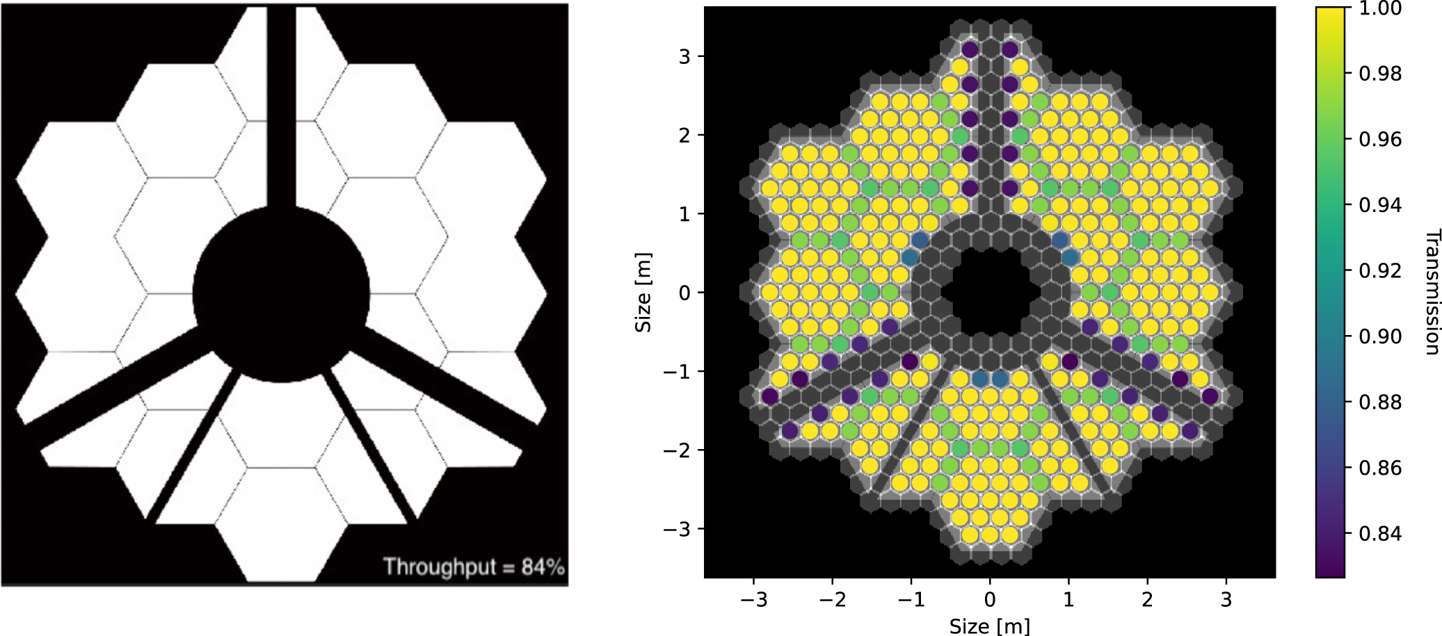
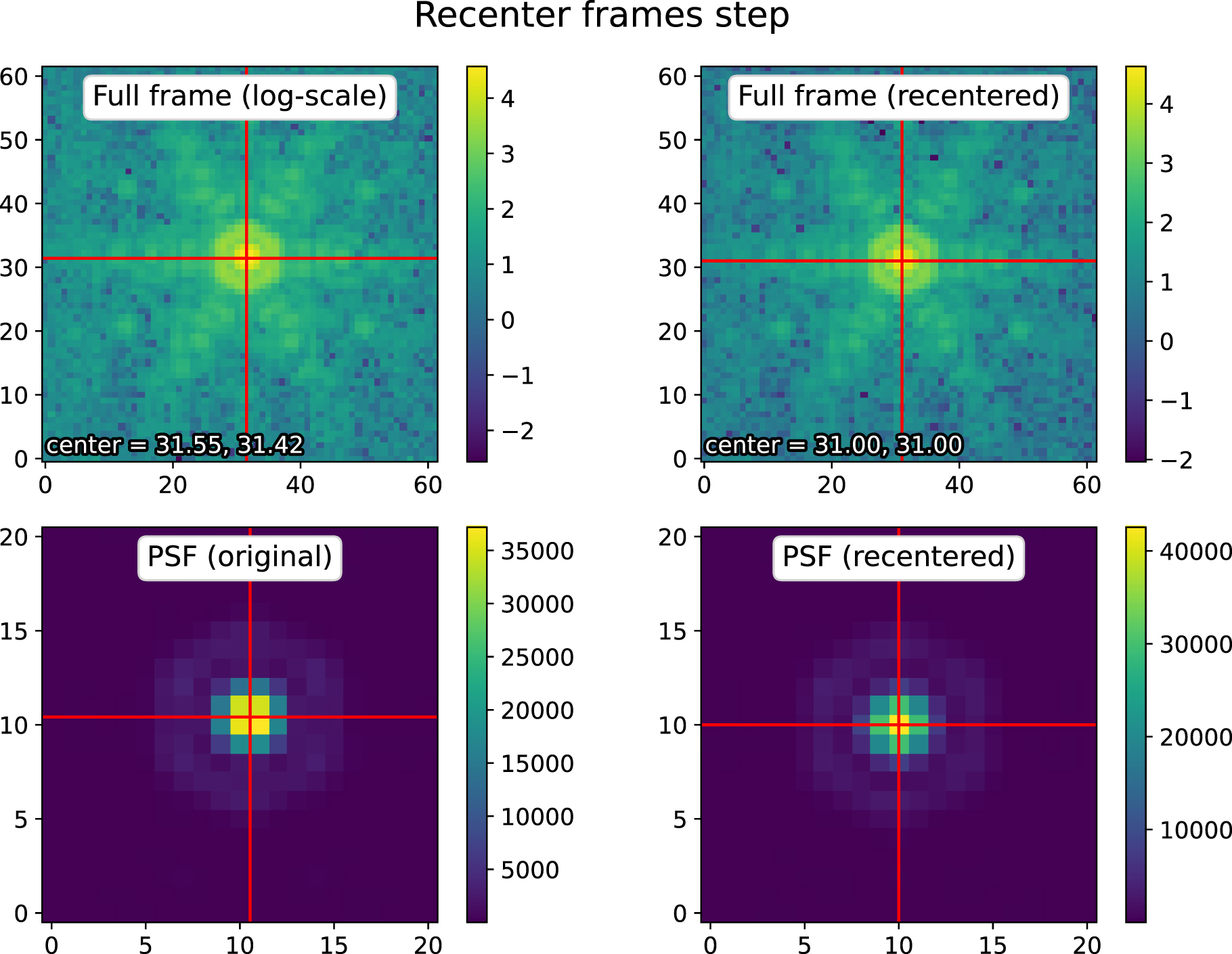
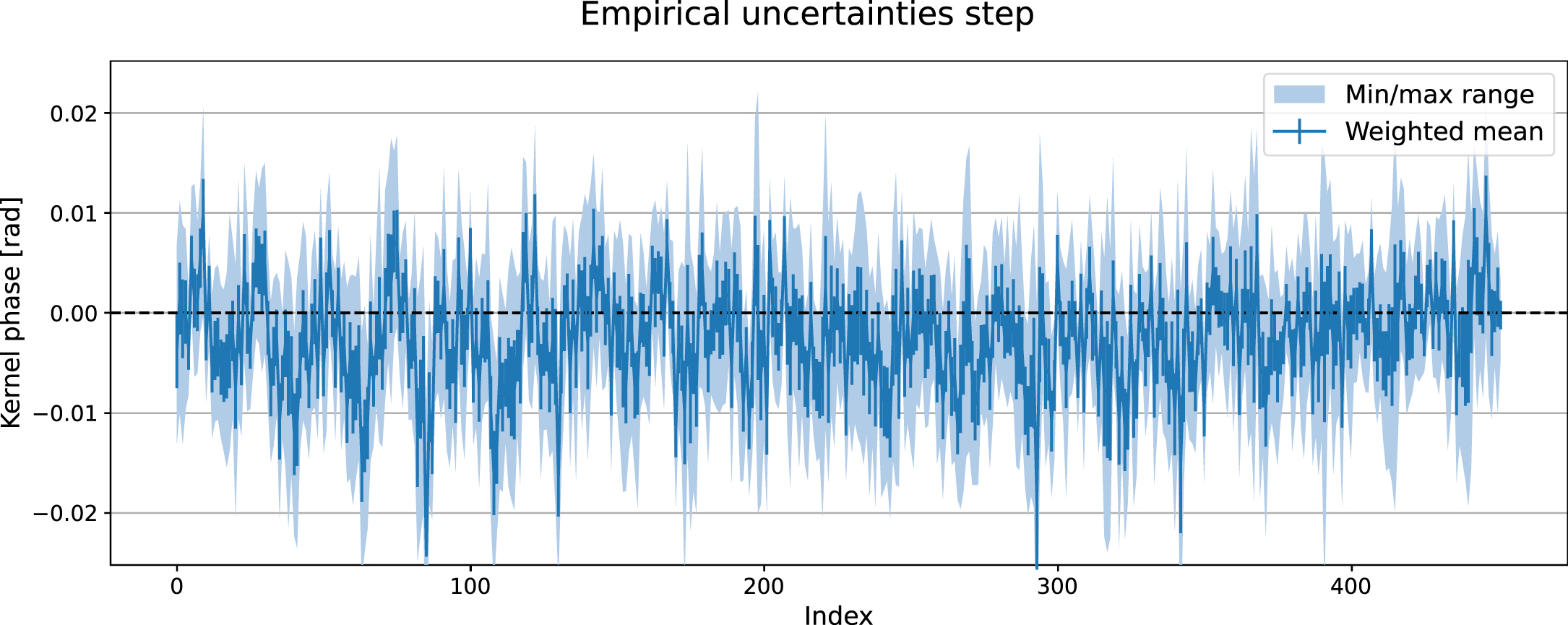
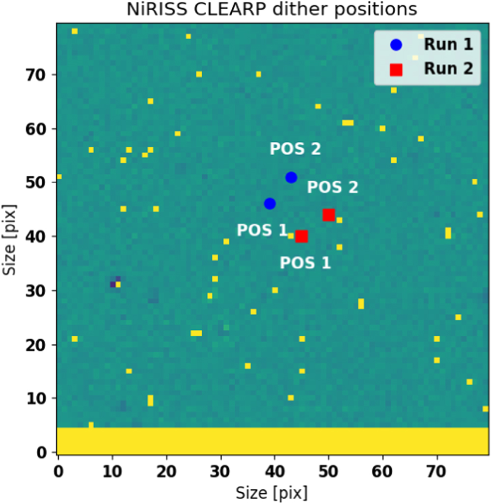
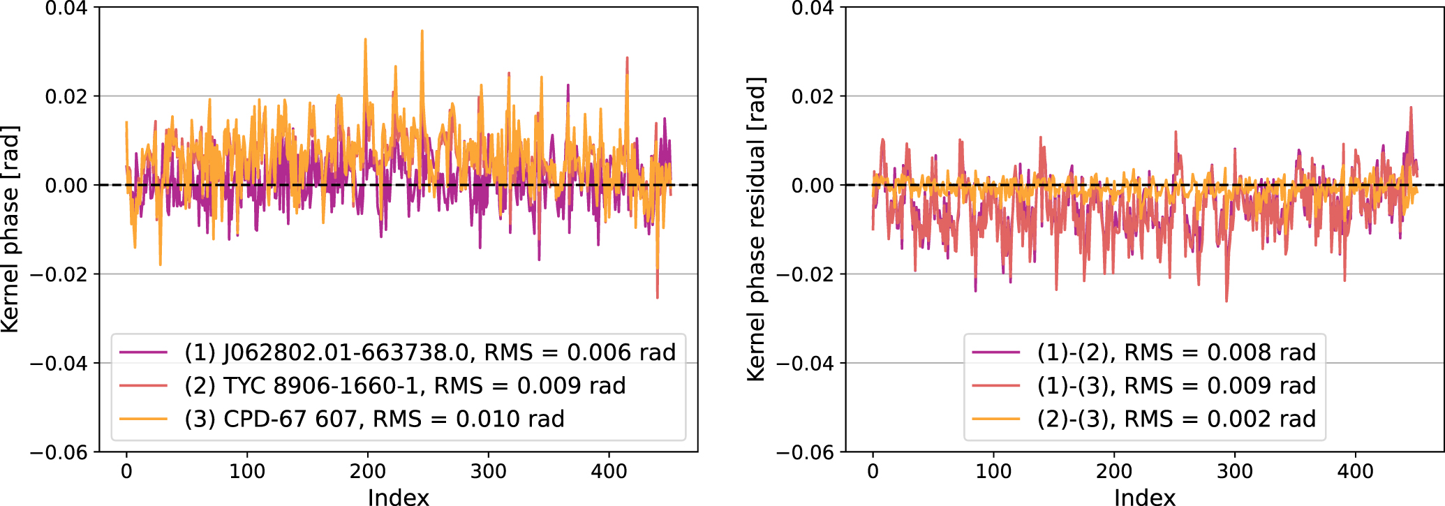
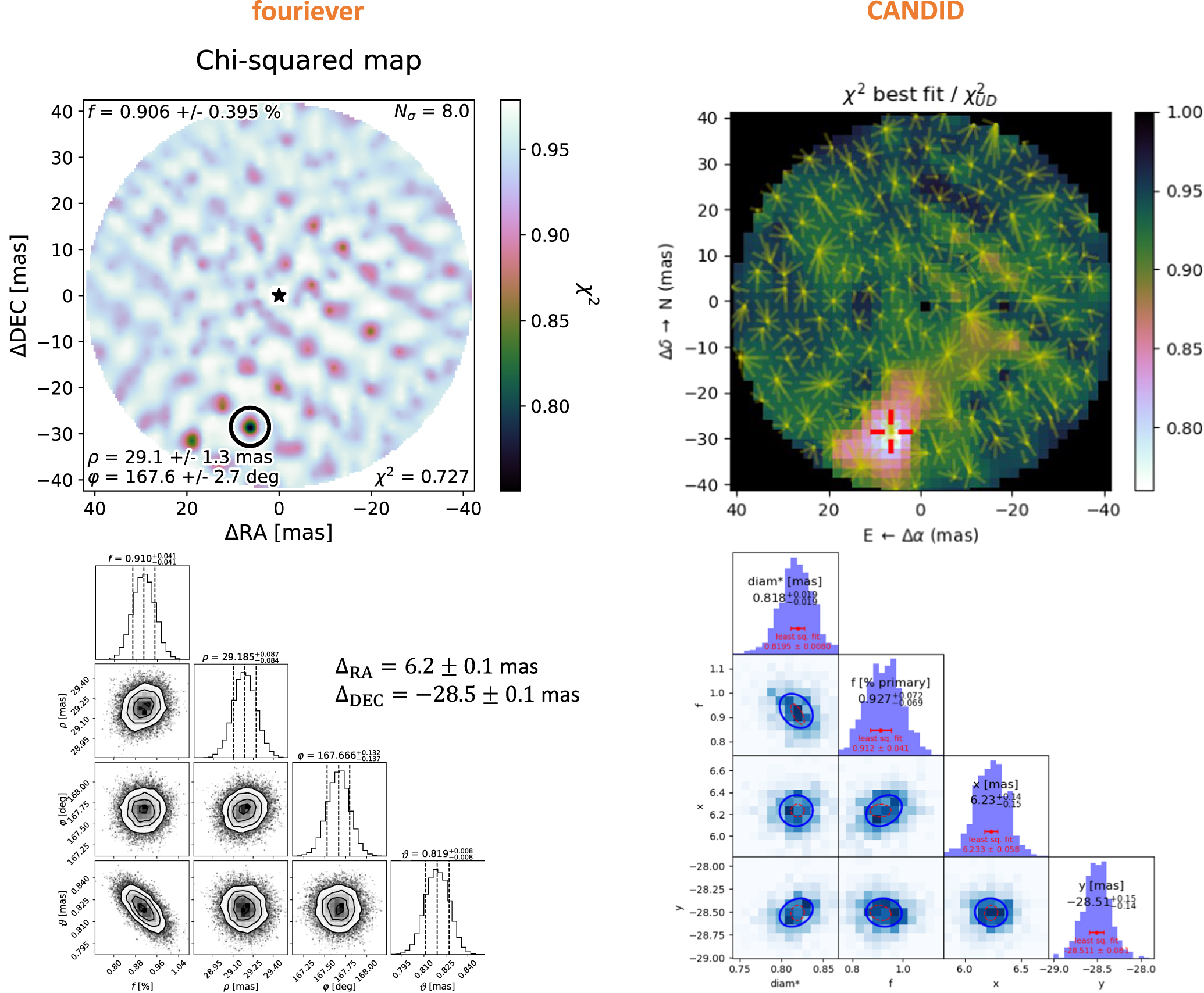
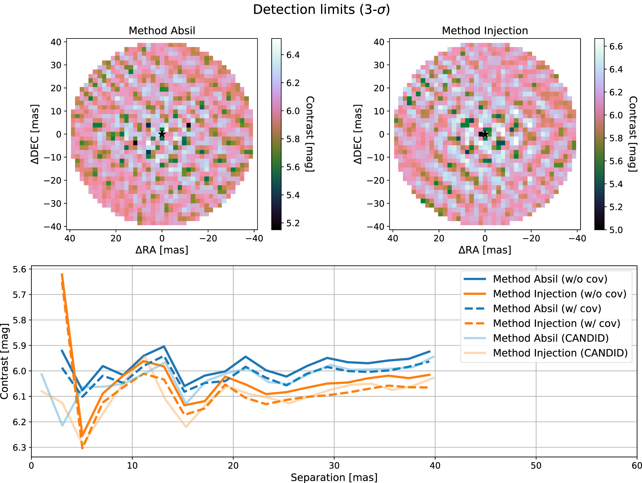
Figure 17. Companion search around 2MASS J062802.01-663738.0, the (supposedly) point-source reference target that was identified to be an outlier in both NIRISS KPI observing runs. The top left panel shows the χ2-detection map and the top right panel shows the data vs. model kernel phase signal as in Figure 9, obtained from a binary model fit to the data from the second run. The bottom panel shows a PSF-subtracted image of 2MASS J062802.01-663738.0 obtained with pyKLIP (20 KL modes). A companion candidate consistent with the one from the kernel phase reduction is clearly detected (white arrow). The image pixel scale is equivalent to the NIRISS detector pixel scale (∼65 mas).
Download figure:
Standard image High-resolution image
Table 4. Tunable Parameters of the Kpi3Pipeline
| Name | Type | Default Value | Allowed Values | Description |
|---|---|---|---|---|
| Bad pixel fixing step | ||||
| skip | bool | False | False/True | Skip step? |
| plot | bool | True | True/False | Make diagnostic plot? |
| bad_bits | list of str | ['DO_NOT_USE'] | See [2] | DQ flags considered bad pixels |
| method | str | 'medfilt' | 'medfilt'/'fourier' | Method to fix bad pixels |
| Recentering step | ||||
| skip | bool | False | False/True | Skip step? |
| plot | bool | True | True/False | Make diagnostic plot? |
| method | str | 'FPNM' | 'FPNM'/'BCEN'/'COGI' | Method to find PSF center |
| trim | bool | True | True/False | Trim images to square size? |
| bmax | float | 6. | Positive non-zero | Maximum baseline [m] for FPNM |
| pupil_path | str | None | Valid path | Path of custom pupil model |
| Windowing step | ||||
| skip | bool | False | False/True | Skip step? |
| plot | bool | True | True/False | Make diagnostic plot? |
| wrad | float | None | Positive non-zero | Windowing function radius [pix] |
| Kernel phase extraction step | ||||
| skip | bool | False | False/True | Skip step? |
| plot | bool | True | True/False | Make diagnostic plot? |
| bmax | float | None | Positive non-zero | Maximum baseline [m] for LDFT |
| pupil_path | str | None | Valid path | Path of custom pupil model |
| Empirical uncertainties step | ||||
| skip | bool | False | False/True | Skip step? |
| plot | bool | True | True/False | Make diagnostic plot? |
| get_emp_err | bool | True | True/False | Use empirically est. errors? |
| get_emp_cor | bool | False | False/True | Use empirically est. correlations? |
Note. The FPNM, BCEN, COGI, and LDFT methods are described in more detail in the XARA documentation (see [1]). [1] = https://github.com/fmartinache/xara, [2] = https://jwst-reffiles.stsci.edu/source/data_quality.html.
Download table as: ASCIITypeset image
Footnotes
- 24
- 25
- 26
- 27
- 28
This target acquisition is accurate to within <0.1 pixels (Rigby et al. 2022).
- 29
- 30
- 31
- 32
- 33
- 34
- 35