

Abstract
This paper reviews parameterized CLEAN deconvolution, which is widely used in radio synthesis imaging to remove the effects of sidelobes from the point-spread function caused by incomplete sampling by the radio telescope array. At the same time, different forms of parameterization and components are provided, as well as methods for approximating the true sky brightness. In recent years, a large number of variants of the CLEAN algorithm have been proposed to deliver faster and better reconstruction of extended emission. The diversity of algorithms has stemmed from the need to deal with different situations as well as optimizing the previous algorithms. In this paper, these CLEAN deconvolution algorithms are classified as scale-free, multi-scale and adaptive-scale deconvolution algorithms based on their different sky-parameterization methods. In general, scale-free algorithms are more efficient when dealing with compact sources, while multi-scale and adaptive-scale algorithms are more efficient when handing extended sources. We will cover the details of these algorithms, such as how they handle the background, their parameterization and the differences between them. In particular, we discuss the latest algorithm, which has been able to efficiently handle both compact and extended sources simultaneously via the deep integration of scale-free and adaptive-scale algorithms. We also mentioned recent developments in other important deconvolution methods and compared them with CLEAN deconvolution.
Export citation and abstract BibTeX RIS
1. Introduction
The invention of the CLEAN deconvolution algorithm has changed radio synthesis imaging and accelerated the development of radio astronomy (Cornwell 2008, 2009). It is a standard component of almost all radio synthesis imaging software. The original CLEAN algorithm was proposed by Högbom (1974), and his fascinating paper (Högbom 2003) has provided the intriguing story behind its creation and development. The basic idea of CLEAN is straightforward and simple : it reconstructs the sky brightness by iteratively identifying point-source components and removing the effects of the point-spread function (PSF). Moreover, it can effectively solve the problem of image blurring caused by sparse sampling, such as due to a limited number of telescopes and Earth-rotation synthesis.
The original CLEAN algorithm is efficient when the objects of interest can be represented by a small number of parameters. That is, the assumption underlying this algorithm is that there are only a few well-separated point sources in the imaging field. In order to improve the deconvolution speed and reduce its errors, some improved algorithms have been proposed, such as the Clark algorithm (Clark 1980) and the Cotton–Schwab algorithm (Schwab 1984). These algorithms, which decompose objects as a set of point sources, are called scale-free CLEAN algorithms. In the early days of the CLEAN algorithm, due to the limited sensitivities of radio telescopes, the measured images could be effectively represented as containing several point sources in a blank area. These algorithms worked well for this particular situation. However, with the development of radio telescope technology, higher sensitivity and more frequency components became available, so that the obtained images contained more objects, including extended emission and complex features. One of the most well-known problems associated with using scale-free algorithms when attempting to deconvolve extended emission is that the deconvolved image may contain different stripes (Clark 1982; Steer et al. 1984); i.e., point-source decomposition and the sidelobes of the PSF together lead to the appearance of stripes in the reconstructed model image. A straightforward way to circumvent this issue is to change the sidelobe level of the PSF, such as adding a delta function to reduce the sidelobe ratio at the center of the PSF's main lobe (Cornwell 1983). This technique proved to be very effective. However, this stripe problem was essentially caused by the use of parametric models in these algorithms, which was addressed by solving the problem of how of pixel dependencies are represented between pixels. Consequently, more researchers chose to use extended components to approximate real sky emission to solve this problem, such as multi-scale algorithms (Cornwell 2008; Rau & Cornwell 2011) and adaptive-scale algorithms (Bhatnagar & Cornwell 2004; Zhang et al. 2016a, 2016b; Zhang 2018a, 2018b).
This paper gives a detailed overview of these three types of algorithms (scale-free, multi-scale and adaptive-scale). In order to better understand them, the deconvolution problem in radio synthesis imaging is introduced in Section 2. The basic flow process employed by CLEAN deconvolution algorithms is described in Section 3, while scale-free, multi-scale and adaptive-scale CLEAN deconvolution algorithms are introduced in Sections 4–6, respectively. A comparison of the parameterization capabilities of each is discussed in Section 7. We then introduce the latest developments of other deconvolution algorithms by way of comparison with CLEAN deconvolution in Section 8, after which we conclude the review in Section 9.
2. The Deconvolution Problem in Radio Synthesis Imaging
Radio synthesis imaging uses dozens of telescopes and Earth-rotation synthesis to measure the spatial frequencies of sky brightness (Taylor et al. 1999; Thompson et al. 2017). This depends on Fourier transform theory and the van Cittert–Zernike theorem which determines the relationship between the sky brightness function and the visibility function (or the spatial coherence function of the electric field).
In the ideal continuous case, the visibility function Vtrue and the sky brightness Itrue are Fourier transform relations,

where F denotes the Fourier transform. In this case, the sky brightness Itrue can be directly obtained by calculating the inverse Fourier transform  of the visibility function, Vtrue as

However, in actual measurements, the visibility function is discretely sampled and always contains noise.

where Vmeasured is the measured visibilities, S is the sampling function, where 1 represents sampled and 0 is unsampled points, and N is the noise in the spatial frequency domain. The sampling function depends on many factors, such as the number of telescopes. In general, the fewer the sampling points, the more significant the PSF sidelobes. Next, the inverse Fourier transform of the measured visibilities is computed to get the dirty image Idirty. According to the convolution theorem, a dirty image is a convolution of the sky brightness and noise with the PSF,

where Bdirty is a Toeplitz matrix in which each row is a shifted version of the PSF which is the inverse Fourier transform of the sampling function S, and  is the noise in the image domain. The details of the celestial image are submerged under the widely spread sidelobes of the PSF. Deconvolution needs to be done to recover the true sky-brightness image from the dirty image, which is performed using inverse Fourier transforms of the noisy and incomplete measurements. Deconvolution essentially implements an estimation of the unsampled points in the visibility (spatial frequency) domain by introducing some restrictions in the image domain. In the field of radio synthesis imaging, the CLEAN algorithm proposed by Jan Högbom is one of the most successful algorithms (Thompson et al. 2017).
3. CLEAN Deconvolution Framework
The Högbom algorithm forms the basis of most CLEAN algorithms, which is based on the Newton method (Rau 2010). The residual peak gives the position and amplitude of the point source. The effects of the PSF sidelobes are removed by iteratively subtracting a scaled PSF at the residual peak position. The potential true image is approximated by iteratively finding point sources in the raw image. This is an iterative deconvolution procedure performed in the image plane. Until 1984, the Cotton–Schwab algorithm (Schwab 1984) formed the basic framework of most existing CLEAN algorithms, which contained two loops: a minor cycle and a major cycle (Rau 2010).
The basic idea of all CLEAN algorithms is to iteratively find the components from a dirty image to approximate the potential true sky brightness, and thereby remove the effects of the PSF sidelobes. The minor cycle is used to find the model's components, and the major cycle is used to correct errors such as gridding errors. Here, we describe the general framework suitable for most CLEAN deconvolution algorithms (Rau 2010), where the minor cycle is nested in the major cycle.
- 1.Find the model components from the current residual image Iiresidual by performing operation T.where i represents the ordinal number of iterations. In some methods, the PSF is often used in the operation T, and this process can be expressed explicitly as
 . For the first iteration, a component is found from the dirty image Idirty.
 - 2.Update the model image by accumulating the components of each iteration while applying a loop gainwhere g is between 0 and 1, which is used to define the step size of fitting and determine the speed of deconvolution.
- 3.Update the residual image in the image plane by removing the effects of the current model component from the latest residual image.Repeat the minor cycle (1)–(3) until one of the top conditions is satisfied. These stop criteria are triggered when reliable signals cannot be extracted from the residual image.
- 4.Predict the current model image to measured data points so that the model image can be directly compared to the measured data.where j is the number of executing major cycles, and A represents the series of operations contained in the degridding procedure.
- 5.Update the residual image by calculating the difference between the measurement visibility function Vmeasured and the predicted visibility function Vjpre, and transform the result to the image plane,where is the residual image in the jth major cycle. Repeat the major cycle (1)–(5) until convergence or the maximum number of iterations is reached.
- 6.Make the CLEAN image Iclean by convolving the final model image Imodel with a Gaussian beam Bclean which is obtained by approximating the main lobe of the PSF,This helps to suppress extrapolated spatial frequencies outside the measured range and hence prevent the model image from overinterpreting the data.
- 7.Calculate the restored image Irestored by adding the final residual image Iresidual to the CLEAN image,This adds the signal remaining in the final residual image to the restored image to ensure the integrity of the signal. However, this step is optional (Taylor et al. 1999). It is worth mentioning that the Fourier transform of the restored image, which is a tapered version of the sky model, is inconsistent with the measured data, so it cannot be used as a model for self-calibration.


In practical implementation, calculation of the dirty image and projection of the predicted model into the ungridded measured points must be taken into account. The measured visibilities need to be weighted and gridded before the dirty image is calculated. However, these steps are beyond the scope of this paper, and we kindly refer the reader the work of Thompson et al. (2017) for more details.
Schwarz (1978) mathematically and statistically analyzed the CLEAN algorithm and provided a proof of its convergence. The most important condition for convergence is that the PSF should be semi-definite positive. Schwarz also pointed out that if the number of independent visibility data points is not less than the number of delta function components used to approximate the potential real sky emission, the CLEAN deconvolution has only one solution. This is equivalent to the Fourier transform of the delta function components fitted to the measured visibilities.
It has been more than 40 yr since the original CLEAN algorithm was put forward, and a large number of variants has been proposed. These algorithms can be roughly divided into three categories: scale-free, multi-scale and adaptive-scale algorithms. Next we will introduce these algorithms in detail.
4. Scale-free CLEAN Algorithms
The main feature of scale-free CLEAN algorithms is that the potential true image is parameterized as a series of delta functions. The model image Imodel is composed of these delta functions.

where  is the sum operator, N is the number of components that make up the model image,
  is the amplitude corrected by a loop gain and
  is the delta function at
  . This model image is used to approximate the potential true image,

where  is the difference between the model image and the potential true image. A smaller indicates that the model image is closer to the potential true image.
The basic process of this kind of algorithm is to find the peak in the current residual image, and then use a loop gain to modify its amplitude to obtain the model component. The next residual image is obtained by subtracting the influence of the current model component. Finally, all model components are accumulated into the model and used to approximate the potential true image.
During the initial stages of development of the CLEAN algorithm, most of the developed permutations were scale-free. It should be mentioned that before the Cotton–Schwab algorithm, the CLEAN-based algorithms were different to the basic framework mentioned in the previous section. Below we introduce some typical algorithms in this class.
4.1. The Högbom Algorithm
The Högbom algorithm (Högbom 1974) is much simpler than the CLEAN framework. In addition to calculating the dirty image, this algorithm only executes the minor cycle in the CLEAN framework. The residual image is updated by subtracting a scaled full PSF containing all sidelobe patterns to remove the contribution of each component. It is generally believed that the closer the residual is to the noise, the closer the model image is to the potential true image. Finding the model is equivalent to minimizing the following objective function,

where  is the Euclidean norm. This algorithm is based on the steepest descent method (Bhatnagar & Cornwell 2004). From the viewpoint of function optimization, the first derivative needs to be calculated to find the update direction of each iteration.

where  and
and  is the peak of the current residual image located at
  in the ith iterations. The peak search of the CLEAN algorithm is not explicitly fitting, but rather it is equivalent to minimize the objective function (Equation (15)) along the gradient direction by iteratively peak searching and subtracting the scale PSF. This is achieved through the first three steps of the CLEAN framework. The result is a series of delta functions with the amplitudes and positions of the peaks in each residual image that make up the model image.
It is well known that the magnitude of the Fourier transform of a delta function is a constant that fills the entire (u, v) plane. This also causes the model's visibility function to be extrapolated out of the measured spatial frequency range. Although a set of delta functions can partly constrain the spatial frequency of the extrapolation, the use of a delta function model to represent extended sources is not physically accurate. This can easily lead to over-interpretation outside the measured spatial frequency range, which is one of the main reasons for using a CLEAN beam to convolve the model.
When deconvolution converges, it is usually assumed that the image mainly contains noise. But when dealing with extended sources, deconvolution usually leaves some signals in the residual image. Therefore the final residual image is often added to the final restored image.Which not only ensures the integrity of the signal in the restored image, but also indicates the level of uncertainty in the restored image.
This algorithm is only performed in the image plane and require a dirty beam image covering twice the extent in each dimension of the image to be deconvolved. Although the calculation is efficient, errors arising from gridding and the fast Fourier transform (FFT) algorithm in the dirty image cannot be corrected.
4.2. The Clark Algorithm
The shift-and-subtraction operation is very effective for calculating the convolution of point sources. However, it is well known that using the convolution theorem for non-point source convolutions is more efficient. In order to reduce the computational complexity of the situation where a large number of delta functions are required to approximate the potential true image, Clark (1980) proposed a new CLEAN algorithm that uses the convolution theorem and FFTs.
The Clark algorithm consists of a minor cycle and a major cycle. Its minor cycle is similar to that in the Högbom algorithm, but the difference is that a beam patch is used instead of the full beam. A beam patch is composed of the main lobe and the maximum sidelobe of the full beam. In the minor cycle, the residual image is updated as follows,

where Bpatch is the beam patch approximated from the dirty beam. The criteria for stopping the minor cycle and starting the major cycle are based on the maximum peak outside the beam patch or a certain number of components being collected. The full beam will be used in the major cycle to remove the effects of the set of point sources identified in the minor cycle from the residual image.

where Bdirty is the full dirty beam. Here the convolution theorem and the FFT are used to quickly calculate the convolution. The full beam also corrects some of the errors caused by the beam patch approximation in the minor cycle to some extent. This algorithm is several times faster than the Högbom algorithm.
4.3. The Cotton–Schwab Algorithm
The Clark algorithm uses the convolution theorem and FFTs to quickly calculate the convolution, and transforms the model image and the dirty beam to the gridded (u, v) plane. These computations greatly accelerate the deconvolution process. At the same time, it also corrects the errors caused by the minor cycle. However, this algorithm still cannot correct the errors caused when calculating the dirty image.
In order to solve this problem, the Cotton–Schwab algorithm (Schwab 1984) was proposed, which is a variant of the Clark algorithm. It performs a major-cycle subtraction on the measured visibility data points,

where Ijmodel is the model image in the jth major cycle, and A maps the model image from the minor cycle onto ungridded measured data points. This algorithm is directly fitted to the measured spatial frequency domain.

In other words, the model prediction is compared with the original data in the data measurement domain. This significantly reduces aliasing noise and gridding errors. Another obvious advantage of this algorithm is that it can separate CLEAN in each field in the minor cycle, and thus the effects of the components of all fields are removed together (Rau 2010). The framework of this algorithm, which uses minor cycles to determine models in the image domain and major cycles to correct errors in the visibility domain, is effectively the same as the standard framework employed by most CLEAN-based algorithms.
The algorithms mentioned above all have been implemented in major radio synthesis imaging software programs such as CASA.5 These scale-free algorithms maintain the idea of the original CLEAN algorithm, which parameterize the radio sky into a series of scaled delta functions. Although experience has shown that these scale-free algorithms also work for extended and complex sources (Taylor et al. 1999; Thompson et al. 2017), as mentioned previously, a widely known problem is that they tend to produce some spurious artifacts such as stripes in the model image when dealing with extended sources. Clark (1982) provided a heuristic explanation of this issue. When scale-free algorithms remove a point source response (a scaled PSF) from the peak of an extended source, the negative sidelobes of the dirty beam generate new extreme values in the following residual image. When searching for the next component, the peaks will be identified as model components in subsequent cycles. The dirty beam pattern is therefore in the residual image of each iteration, resulting in the same or similar fringe spacing in the model image due to the sidelobes of the dirty beam. As the sidelobe level increases, the stripes become more pronounced.
There are many ways to solve this problem. As this problem is caused by the sidelobes of the dirty beam, the general idea is to start with the sidelobes. For example, a small loop gain can be used so that the residual image is reduced by the sidelobes, thereby suppressing the formation of stripes in the model image. As mentioned above, the method (Cornwell 1983) is to add an artificial "spike" at the center of the main lobe of the dirty beam to compress the sidelobes and in turn reduce/remove the stripes from the model image. Another idea is to directly suppress the stripes in the model image (Palagi 1982; Cornwell 1983). For example, Cornwell (1983) added a smooth regularization term based on model images to the objective function to achieve the suppression of stripes. Steer et al. (1984) attempted to solve this problem by using a group of delta functions as model components above the threshold of the current residuals. A more effective method is to use a scale-sensitive basis to parameterize the radio sky, which is the subject of the next two sections.
5. Multi-scale CLEAN Algorithms
Since the early days of the development of radio interferometry, the resolution and sensitivity of telescope arrays have increased significantly, which has resulted in countless images of astronomical targets showing extended and complex structures being obtained. As mentioned previously, if scale-free algorithms are used to process these sources, spurious artifacts such as stripes are often generated. This is essentially because scale-free models do not express extended and complex features well. So while scale-free models can effectively express well-separated point sources, extended and complex features are ineffectively represented by a set of delta functions. In other words, using a scale-free model to approximate extended and complex features is physically inaccurate. Instead, a natural approach is to use a model that provides a more physical description of extended and complex features to represent them at different spatial scales. This can be achieved by using a multi-scale model to parameterize such features,

where k is the ordinal number of each model component, and  is the kth component with amplitude a, position l and spatial scale s. Note that a refers to the amplitude after being scaled by a loop gain. For a multi-scale model, s is a user-specified and limited number of spatial scales. Obviously, a multi-scale model parameterizes the radio sky into a finite number of spatial scale combinations. Such a model can represent the correlation between pixels and provide strong constraints for estimating unmeasured spatial frequency points. In a multi-scale model, scale basis functions can effectively represent extended and complex features, thereby eliminating the stripes that occur in a scale-free model and further obtaining more noise-like residuals. Some examples of multi-scale CLEAN algorithms are presented in the following subsections.
5.1. The Cornwell–Holdaway Algorithm
In this algorithm, the radio sky is parameterized as a combination of some tapered and truncated parabola with limited and different spatial scales. The component shapes are controlled by the following function f (Cornwell 2008),

where s is the size of the scale used to model the component and  is a prolate spheroidal wave function (refer to Schwab (1978, 1980) for more information). In this algorithm, the components are determined by finding the global peaks in the modified residual images and by combining the corresponding scale information. Different scales are iteratively found at different locations to form complex features to approximate any potential true emission. Here, each scale is essentially a convolution of a scaled delta function
  and a normalized scale function
  ,
,

A sub-image of at a given scale is a convolution between a series of scaled delta functions centered at different positions and this scale function. By combining sub-images at different scales, a model image can be constructed to approximate the potential true emission,

where Ns is the total number of components that make up the model image, which actually has only s different scales in Ns. In order to reconstruct compact sources, s = 0 is allowed, that is,  is a delta function and
  is a tapered, truncated parabola of scale s. If all the scales are s = 0, then the emission is decomposed into a series of delta functions just as a scale-free model. These sizes and number of scales are determined by the user, which has both flexibility and difficulty in determining the configuration.
In this algorithm, the scale found by the matching filtering is biased to smaller scales before entering the model image and updating the next residual image. A valid empirical formula achieves this bias,

where sbias is the biased scale, s is the scale found by the matching filtering, and smax is the user-specified maximum scale. This bias can achieve better reconstruction of extended sources (Cornwell 2008). For example, if there is a strong point source and a small, weak extended emission around it, the matching filtering will detect a large scale, and if no bias is used, a large scale component will be subtracted from it. Then the strong point source in the following residual image will be maintained and a large negative bowl structure around the strong point source will be produced at the same time. The elimination of the negative structure requires many components (iterations).
In scale-free CLEAN algorithms, if the loop gain for extended emission is much greater than 0.1, then component-estimation errors will result, which requires a large number of iterations to correct. Just like a scale-free CLEAN algorithm, the Cornwell–Holdaway algorithm also uses a loop gain to optimize the magnitude of each component in order to correct the errors caused by component estimation. Fortunately, the loop gain of the Cornwell–Holdaway algorithm has a wide range of choices,where a loop gain of 0.5 or more can produce a good reconstructed image.
This algorithm has been implemented in CASA as in tclean task of CASA by deconvolver = "multiscale," and it has been successfully applied in many published data sets (e.g., Rich et al. 2008).
5.2. The Grisen–Moorsel–Spekkens Algorithm
The basic idea of the Grisen–Moorsel–Spekkens algorithm is consistent with that of the Cornwell–Holdaway algorithm (Greisen et al. 2009); that is, an image is parameterized as multiple scale basic functions. However, scale basis functions have many choices when certain conditions are met (Cornwell 2008). The Grisen–Moorsel–Spekkens algorithm uses a two-dimensional Gaussian function to model the components instead of the tapered, truncated parabola in the Cornwell–Holdaway algorithm.

where xn and yn are the mean values of the x and y axes respectively, and  is the standard deviation. The sky emission is approximated by a set of Gaussian functions whose widths are
  , which are specified by the user.

In the Cornwell–Holdaway algorithm, pre-calculating the cross-terms between the scales specified by the user makes it possible to find the optimal component at all scales in each minor cycle. This is done without recomputing the smoothed residual image in the spatial frequency domain. However, the cross terms in the Cornwell–Holdaway algorithm are not calculated in this algorithm and only one scale is computed during each minor cycle. Like the Cornwell–Holdaway algorithm, the Grisen–Moorsel–Spekkens algorithm uses a scale bias term as follows to suppress the spatial scales to reduce errors,

where  . This is equivalent to using a Gaussian area to normalize the residual images (Rau 2010).
This algorithm is available in AIPS,6 and has been successfully applied to many published data sets (Thilker et al. 2002; Clarke & Ensslin 2006; Momjian et al. 2006; Kent et al. 2009).
5.3. The Cornwell–Rau Algorithm
The scale biases in the Cornwell–Holdaway and Grisen–Moorsel–Spekkens algorithms are equivalent to normalizing the smoothed residual images (Rau 2010). The Cornwell–Rau algorithm (Rau & Cornwell 2011) achieves this goal through a Hessian matrix ![$[{H}^{\mathrm{peak}}]$](https://content.cld.iop.org/journals/1538-3873/132/1010/041001/revision1/paspab7345ieqn22.gif) . Each element of the Hessian matrix
. Each element of the Hessian matrix  represents the sum of the uv-tapered gridded imaging weights,

where ![${tr}[M]$](https://content.cld.iop.org/journals/1538-3873/132/1010/041001/revision1/paspab7345ieqn24.gif) is the trace of matrix
is the trace of matrix ![$[M]$](https://content.cld.iop.org/journals/1538-3873/132/1010/041001/revision1/paspab7345ieqn25.gif) , Ts is an uv-taper function of scale s,
, Ts is an uv-taper function of scale s,  denote the indices of the scale basis functions, which are tapered truncated parabolas, S is the sampling function,
  is the inverse of S, W is the weights, and Ns is the number of scale basis functions. The normalization of the Hessian matrix is useful for the case of overlapping components at different spatial scales. This makes estimating the total flux of the component more accurate than the Cornwell–Holdaway algorithm. A measure of the area of the main lobe of the PSF at different spatial scales corresponds to the diagonal elements of this Hessian matrix. When calculating the principal solution, these normalization methods are equivalent to using the diagonal elements of the Hessian matrix. This work (Rau 2010) has carried out detailed development of the theory of CLEAN algorithms through linear algebra. The Cornwell–Rau algorithm has been combined with multiscale CLEAN to solve the problem of wideband imaging, and has become a commonly used algorithm, such as in the tclean task of CASA by deconvoler = "mtmfs."
5.4. The Offringa–Smirnov Algorithm
Like the Cornwell–Rau algorithm (Rau & Cornwell 2011), the Offringa–Smirnov algorithm (Offringa & Smirnov 2017) made some changes to the multi-scale algorithm (Cornwell 2008), which was extends to the wideband case using the joined-channel method, and was verified using real data. The minor cycle of this algorithm is similar to that of the Clark algorithm (Clark 1980), i.e., there is subminor cycle. In the subminor cycle, only one scale is considered and multiple iterations are performed at the current scale. This method no longer seeks the sparsest solution under the enumerated scales with an increasing number of components, which reduces the computational load. A tapered quadratic function and a Gaussian function are implemented as scale basis functions. In order to implement this modified minor cycle, a new scale-bias function was also proposed. With this automatic scale-dependent masking technique, a deeper deconvolution can be performed.
While achieving similar results, the algorithm's minor cycle is more than an order of magnitude faster than the Cornwell–Holdaway algorithm (Cornwell 2008) in the single-frequency mode, and 2–3 orders of magnitude faster than the Cornwell–Rau algorithm (Rau & Cornwell 2011) in multi-frequency mode.
5.5. Other Implementations
There are other implementations, such as WSCLEAN (Offringa et al. 2014) and the Hybrid Matching Pursuit and sub-space optimization algorithms applied to the wideband widefield cases (Tasse et al. 2018). These multi-scale algorithms use scale basis functions to parameterize their corresponding features at multiple scales to represent the sky emission. Compared to scale-free algorithms, these algorithms can extract extended emission more efficiently. In general, multi-scale algorithms first extract large-scale features, and then gradually find smaller-scale features. This is in constrast to scale-free algorithms, which extract pixel details and scale features are broken into points.
The Wakker–Schwarz multi-resolution algorithm (Wakker & Schwarz 1988) can be classified in the category of multi-scale deconvolution. Unlike the multi-scale algorithms mentioned previously, it first extracts scale features from the lowest resolution and then extracts finer structures from higher resolution images. It considers a single scale in each minor cycle instead of processing all scales in each minor cycle, as performed by the Cornwell–Holdaway algorithm and the Cornwell–Rau algorithm. Another algorithm similar to the Wakker–Schwarz multi-resolution algorithm is the wavelet CLEAN agorithm (Horiuchi et al. 2001), which uses wavelet transforms to achieve multi-resolution reconstruction. However, these two algorithms still perform a series of Högbom minor cycles, which parameterizes the radio sky as a set of delta functions. From this perspective, they are also scale-free CLEAN algorithms.
In general, multi-scale algorithms have greatly improved the performance of extracting extended and complicated sources from radio images (Bhatnagar & Cornwell 2004). However, scale selection is limited to the chosen enumerated scales and there is no theory or method that can help guide the selection of better components. All component scales must be consistent with pre-specified scales. Features that differ from the pre-specified scale will be broken, which requires more iterations to correct. This problem is solved by finding ways to scale adaptively, as well be described in the following section.
6. Adaptive-scale CLEAN Algorithms
Scale-free CLEAN algorithms parameterize the radio sky into a series of point sources, while multi-scale CLEAN algorithms parameterize sky emission into a series of specified scales. The scale-free CLEAN algorithm can be seen as having only one specified scale, which is 0. However, the sky emission scale cannot be determined in advance. When the scale of a feature is inconsistent with the specified scale, the feature will be broken into many smaller scales. Obviously this is not an optimal representation. Instead, when adaptive-scale CLEAN algorithms parameterize the sky, the scales are not limited to a few specified scales, but are adaptively found according to the features of the sky emission. The adaptive scale-based model can be expressed as follows,

The optimal parameters are obtained by explicit fitting, which allows the scale to change adaptively. This fitting is done by minimizing the following objective function,

The update direction is needed to calculate the derivative of  for these parameters,

This approach effectively considers the uncertainty of the sky emission scales. The spatial correlation length (a measure of the scale) is a stronger separator of signal and noise (Bhatnagar & Cornwell 2004), which allows the model to better reflect the true potential sky emission.
6.1. The Bhatnagar–Cornwell Algorithm
This adaptive scale pixel decomposition algorithm (also called the Asp-Clean algorithm) (Bhatnagar & Cornwell 2004) finds the optimal component at the "energy" peak position of the current residual image, which is achieved by blurring the current residual image using several Gaussian functions and then finding the global peak. The number of model parameters monotonically increases with the number of iterations. If all the model parameters are fitted in each minor cycle, the computational complexity will be very large for a complex image containing several hundred components. Therefore, only one active-set is optimized at a time rather than optimizing all components simultaneously,

where  and
and  are convolutions, and only some of the parameters in
  can be changed, that is, the part related to the active-set. The number of components in an active-set also determines the dimensions of the search space in each iteration. The active-set of components is adaptively determined in each iteration, including how many components are used each time.
In the Bhatnagar–Cornwell algorithm, the length of the parameters' derivatives need to be calculated,

where ∇i is the derivative operation of the parameters of the ith component. The method of determining the active-set is simple. First, Li is computed before each fitting iteration, then a threshold L0 is used to determine if a component is in the active-set. If Li is less than L0, then this component will be removed from the active-set. The threshold L0 is determined as follows,

where λ is a hyperparameter that affects the size of the active-set, and has an experimental value. The non-orthogonality of the search space of this algorithm solves the problem of model representation in which the pixels of the extended feature are not independent.
6.2. The Zhang et al. Algorithm
The Bhatnagar–Cornwell algorithm finds the optimal model components by minimizing an objective function. However, it is a time-consuming process. In a typical function-optimization process, finding an optimal result often requires a large number of iterative calculations. Zhang et al. (2016a) identified the most time-consuming part of the Bhatnagar–Cornwell algorithm, and henced proposed a faster algorithm known as the Asp-Clean2016 algorithm.
In this algorithm, model components are found by minimizing a different objective function,

where  containing the amplitude
  , position
  and width
  , which is a fitted Gaussian function that contains a model component whose parameters are obtained using the Levenberg–Marquardt optimization algorithm (Marquardt 1963). After each fitting convergence, the potential components can be extracted from IicGauss by an analytical method. The width of the model component contained in IicGauss is calculated as follows,

where  ,
,  and
and  are the widths of model component Iicomponent, IicGaussian and the Gaussian beam, which is approximated from the PSF, respectively. After obtaining the widths of the current model components, the magnitude
  of each component is estimated as follows,

where  and
and  are the amplitudes of the Gaussian beam and IicGaussian, respectively.
Analytically deconvolving the PSF allows the convolution calculations in the objective function to be removed, which results in a significant reduction in computational effort relative to the Bhatnagar–Cornwell algorithm. The quality of the imaging obtained with both algorithms is similar.
6.3. The Fused-Clean Algorithm
Scale-free algorithms can represent well-separated point emission very well and their computational methods are very effective; however, such algorithms are not optimal for the representation and calculation of extended and complex emission. Although multi-scale and adaptive-scale algorithms already include a zero-scale (i.e., delta functions) for approximating compact emission, their computational methods are not very efficient. The fused-Clean algorithm (Zhang 2018a) was proposed, which combines the Högbom algorithm and the Asp-Clean2016 algorithm.
The fused-Clean algorithm automatically triggers Högbom minor cycles and Asp-Clean2016 minor cycles according to different situations. When the initial scale is less than a pre-set threshold (e.g., 1.2 times the width of the PSF) or small scales occur frequently in recent iterations (e.g., the scales of five components during the previous 10 iterations were less than 1 pixel), then the minor cycle of the Högbom algorithm is triggered. Once the minor cycle of the Högbom algorithm is triggered, it will be executed many times. The number of iterations executed each time increases with the number of triggers, which works well when the following relationship is satisfied,

where ttn is the number of the minor cycles used by the Högbom algorithm executed at the tnth trigger.
The Asp-Clean2016 algorithm is almost always preferred when there is strong extended emission in the residual image. As the deconvolution deepens, the signal in the residual image gradually decreases, and many scale-free emissions will appear. Then the Högbom algorithm is called to reconstruct the scale-free emission. The scale-adaptive performance of the Asp-Clean2016 model effectively separates emission and noise, whereas the Högbom–Clean algorithm can effectively reconstruct dense emission. The combination of these two algorithms ensures the effective separation of the emission and noise and also accelerates the entire deconvolution process. In general, the fused-Clean algorithm is several times faster than the Asp-Clean2016 algorithm. This fusion represents an incremental improvement to the Asp-Clean2016 algorithm and is a useful step toward making the Asp-Clean algorithm more practically usable.
There are also other scale-adaptive algorithms, such as the Algas-Clean algorithm (Zhang et al. 2016b; Zhang 2018b). This algorithm not only has the ability to perform scale adaptation, but it also achieves accurate reconstruction of the signal through a shape-dependent adaptive loop gain scheme.
7. Comparison of Parameterizations
To verify the performance of different parameterized CLEAN algorithms, we simulated, using CASA, an EVLA observation of the supernova remnant G55.7+3.4 obtained by Bhatnagar et al. (2011), which contains strong and weak point sources as well as extended emission. The noise in this actual image was removed to form the "true" model, which is shown in Figure 1(a). The observation parameters are the same as those used by Zhang et al. (2016a). The dirty image of this simulated observation is shown in Figure 1(b). The deconvolution results of these four algorithms are shown in Figure 2 and Table 1. The root mean square (rms) of the source region in each residual images was calculated (Table 1), and it was found that the adaptive-sacle CLEAN achieved a lower rms, which indicates that this type of algorithm can more effectively extract signals from dirty images. From the perspective of the model's total flux, the restored total flux when using the multi-scale and adaptive-scale CLEAN was greatly improved compared to the traditional scale-free algorithms (i.e., the total flux of the clean image before the simulation observation was about 1.40 Jy). In the model image produced by the Cotton–Schwab algorithm, as shown in Figure 2(a0) which is composed of 60,000 scaled delta functions, it can be seen that there is a significant difference between the model image and the original image. This is mainly caused by the fact that the scale-free parameterization cannot accurately represent the extended emission. This can also be confirmed by the large number of residual correlation signals contained in the corresponding residual image shown in Figure 2(a1). The model image produced by the Cornwell–Holdaway algorithm shown in Figure 2(b0) contains 15,000 components of different specified scales, and the model image is significantly closer to the original image than the model image produced by the Cotton–Schwab algorithm. The improvement in performance stems from the fact that multi-scale parameterization has a strong ability to express extended emission. The model image produced by the Asp-Clean2016 algorithm shown in Figure 2(c0) has 3000 scale components and the corresponding residual image shown in Figure 2(c1) has fewer signal residuals. The quality of this reconstruction is significantly improved compared with the former. The image reconstruction quality of the fused-Clean algorithm is basically consistent with that of the Asp-Clean2016 algorithm, as both algorithms use an adaptive-scale approach to parameterize the sky. The difference between them is that the fused-Clean algorithm uses the Högbom–Clean algorithm to reconstruct the dense emission, which makes the reconstruction speed much faster. Our test showed that the fused-Clean algorithm is six times faster than the Asp-Clean2016 algorithm. This is an important step in the practical usability of the adaptive-scale parameterized CLEAN algorithm.

Figure 1. (a) the supernova remnant G55.7+3.4 image, (b) the corresponding dirty image.
Download figure:
Standard image High-resolution image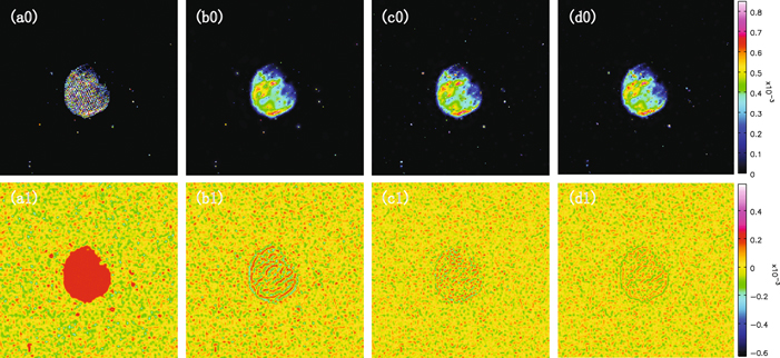
Figure 2. Deconvolution results of the supernova remnant G55.7+3.4 image. From left to right in columns are from the Cotton–Schwab, Cornwell–Holdaway, Asp-Clean2016 and fused-Clean algorithms, respectively. From top to bottom in rows are the model images and the residual images, respectively.
Download figure:
Standard image High-resolution image
Table 1. Numerical Comparison of Different Deconvolution Algorithms for "G55.7+3.4" Simulation
| CoS | CH | Asp2016 | fused | |
|---|---|---|---|---|
| Compact Components | 60,000 | - | - | 3042 |
| Diffuse Components | 0 | 15,000 | 3000 | 761 |
| rms (10−4 Jy) | 1.85 | 1.09 | 0.87 | 0.76 |
| Model Totalflux (Jy) | 1.28 | 1.42 | 1.41 | 1.41 |
Note. CoS, CH are short for the Cotton–Schwab algorithm, the Cornwell–Holdaway algorithm, respectively. Some compact components may be in these model images deconvolved by the Cornwell–Holdaway and Asp-Clean2016 (here Asp2016) algorithm, but it is hard to count them. So the symbol "-" is used for them. rms here means the rms of the source region in these residual images.
Download table as: ASCIITypeset image
Overall, adaptive-scale parameterized CLEAN algorithms have been significantly enhanced in terms of processing extended and complex emissions. The advancements made by these algorithms also promote the concurrent and rapid development of radio astronomy. For additional details beyond the CLEAN parameterization, please refer to Taylor et al. (1999).
8. Comparison to Other Algorithms
Limited spatial-frequency measurements cause the measurement equation (Equation (3)) to yield nonunique solutions. Therefore, some prior information needs to be supplied to obtain the optimal solution. For example, CLEAN-based algorithms use scale information to select a solution. Compressive sensing (CS) algorithms (Candes & Wakin 2008; Wiaux et al. 2009a, 2009b; McEwen & Wiaux 2011) instead use a sparse-representation prior, while maximum entropy methods (MEM) (Narayan & Nityananda 1986) often assume that the sky brightness is positive. Mathematically, CLEAN algorithms are a typical inverse model, while CS-based methods often use sparse regularization (e.g., Wiaux et al. 2009a, 2009b; Akiyama et al. 2017b) and MEM frequently use image entropy or smooth regularization (e.g., Narayan & Nityananda 1986; Chael et al. 2016; Kuramochi et al. 2018),which are typical forward models. Forward models are used less frequently than CLEAN in radio synthesis imaging (EHT Collaboration et al. 2019), however they have recently been extensively developed for the Event Horizon Telescope (EHT) imaging (Honma et al. 2014; Bouman et al. 2016, 2018; Chael et al. 2016, 2018; Ikeda et al. 2016; Akiyama et al. 2017a, 2017b; Kuramochi et al. 2018; EHT Collaboration et al. 2019).
8.1. Compressive Sensing
CS theory (Candes 2006; Candes & Wakin 2008) tells us that when a signal is sparse, or can be sparsely represented under a given basis function dictionary, the signal can be reconstructed with much less sampling than required by the Nyquist–Shannon theory. Sky brightness is sparse in the image domain for compact sources, and it is also sparse in a basis function dictionary when the sky brightness contains diffuse sources. Most of these methods use L1 norms, which can achieve a more sparse solution, with a certain regularization. Because the Fourier domain and the image domain are perfectly incoherent (Candes et al. 2006), CS can be applied directly to the image domain to reconstruct compact sources. For example, the Partial Fourier based CS deconvolution method (Li et al. 2011) applies the L1 norm in the image domain,

where M is the measurement matrix. This method can effectively reconstruct compact sources. Wavelet transformations are often used to achieve sparse transforms of diffuse sources in radio astronomy. Many studies are based on wavelet transforms such as the undecimated wavelet transform (Starck et al. 2007), which use different strategies or objective functions to apply CS during the deconvolution of diffuse radio images, such as Li et al. (2011), SARA (Carrillo et al. 2012), PURIFY (Carrillo et al. 2014), (Garsden et al. 2015), MORESANE (Dabbech et al. 2015) and SASIR (Girard et al. 2015).
The emergence of CS-based deconvolution (e.g., Pratley et al. 2018) has provided a new alternative image reconstruction scheme for radio synthesis imaging which is basically different to the schemes used by CLEAN algorithms (Wiaux et al. 2009a). The CLEAN algorithms yield high-quality reconstructed images by introducing scale priors and combining L2 norms, while CS methods use sparse priors that are combined with L1 norms and a regularization to obtain high-quality images for different cases. CS methods can reconstruct rich structures that contain sharper and more details in specific and simple scenarios. However, most of them have been validated only for relatively simple test samples, and they are deemed unstable for application to real data (Offringa & Smirnov 2017).
8.2. MEMs
MEMs (Cornwell & Evans 1985; Narayan & Nityananda 1986; Cornwell et al. 1999; Akiyama et al. 2017b; EHT Collaboration et al. 2019) are technically similar to CS methods in that they often introduce a priori information through regularization. This regularization is implemented by an entropy function, which is a function of the model emission reconstructed from the dirty image. During the reconstruction of an image, the entropy function is maximized by making the model's visibilities fit mostly to the measured visibilities. Many studies have discussed the construction of entropy functions from theoretical and philosophical perspective, and a large number of these algorithms are based on Bayesian statistics. Some common entropy functions  have been described by Thompson et al. (2017), such as


MEM still needs to minimize the errors resulting from the measured visibilities and model visibilities. The difference relative to CS methods is that MEM uses an entropy function instead of L1 norms.
Both MEM and CLEAN have been used to estimate the true sky emission from incomplete noisy measurements. However, CLEAN is more straightforward and easier to implement. There are some differences between these two types of algorithms: MEM employs explicit optimization, which is not the approach used by most CLEAN algorithms. Moreover, MEM requires an initial model, but CLEAN algorithms do not. MEM images tend to be smooth while CLEAN images show more details. Additionally, MEM is not good at point-source reconstruction, but multi-scale and adaptive-scale CLEAN algorithms are capable of processing point sources and extended sources simultaneously.
9. Conclusions
For more than 40 yr, the development of the CLEAN algorithm has greatly promoted the development of radio astronomy. The development path of the CLEAN algorithm is also very clear. From the initial stage of scale-free parameterization, through multi-scale parameterization, to the most recent adaptive-scale parameterization, recent CLEAN algorithms are able to process extended and complex celestial images better and faster. Such a development path is also consistent with the development of radio astronomy, especially with the development of radio interferometric arrays. With the advent of new radio technology, more complex celestial image acquisition methods will become commonplace, which will undoubtedly promote the concurrent evolution of the CLEAN algorithms for adaptive-scale parameterization. Indeed, one of the main reasons for the success of CLEAN-based algorithms is likely their parameterization mechanism, which gives users enough opportunities to implicitly introduce some a priori information through parameter tuning, which further aids converges to a solution consistent with the data.
In scale-free CLEAN algorithms, a celestial image is parameterized into a series of scaled delta functions. Scale-free parameterization is very effective for well-separated point sources. However, for extended and complex celestial images, the dependence between pixels is not well expressed. That is to say, scale-free parameterization considers pixels to be independent, which does not match reality in the sense that pixels containing an extended source are not independent, which leads to the algorithms' inability to reconstruct extended and complex emission.
To solve this problem, multi-scale parameterization was devised. In multi-scale CLEAN algorithms, a celestial image is parameterized into a set of multiple scales. The scale basis function can effectively express the dependence between pixels containing emission at the same corresponding scale. The problem with multi-scale parameterization, however, is that the scales need to be specified in advance, and they are limited. If the scale used to represent the celestial image is not within the specified scale list, the scale will be broken into multiple scales. This limits the exact recovery of the image.
In order to improve the quality of image reconstruction, adaptive-scale parameterization naturally developed. In adaptive-scale parameterization, the scales are not specified in advance, but instead depend on the observed celestial image itself. This corresponds well to the fact that the scales of a celestial image are uncertain and cannot be predicted beforehand. This allows the adaptive-scale CLEAN algorithm to have the best reconstruction quality. At present, these adaptive-scale algorithms are still developing rapidly and have not been implemented yet in public astronomical data processing software such as CASA.
Over the years, the development of CLEAN algorithms has been more about how to better reconstruct extended and complex celestial images. Currently, CLEAN algorithms handle extended and complex celestial images very well. However, CLEAN algorithms still have a huge room for development, especially for algorithm development of different instruments. It is worth mentioning that CLEAN algorithms are suitable for application to small or medium scale data. When SKA7 and ngVLA8 are built, the amount of observational data will increase so much that new CLEAN algorithms or other deconvolution algorithms will need to be developed to solve these big data problems.
Overall, CLEAN-based algorithms are straightforward and easy to implement. They are usually significantly faster than more complex sparse optimization or CS algorithms (Offringa & Smirnov 2017). In addition, CLEAN-based algorithms are easy to parallelize, e.g., in a faceting scheme (van Weeren et al. 2016). CLEAN-based algorithms have been developed in depth and have been fully tested in terms of solving problems related to widefield and wideband imaging (Rau & Cornwell 2011; Bhatnagar et al. 2013), and they can be called in the widely used CASA package. However, other algorithms are more tested in relatively simple scenarios such as narrow-band imaging (Offringa & Smirnov 2017).
Although CLEAN-based algorithms are the most widely used, other algorithms are also use in radio synthesis imaging. For example, Offringa & Smirnov (2017), Tasse et al. (2018) are used in MeerKAT, LOFAR and MWA imaging. Some methods are widely used in some specific application scenarios. For example, a large number of sparse deconvolution techniques and Bayesian statistics-based deconvolution techniques were developed for EHT imaging of black holes (Honma et al. 2014; Bouman et al. 2016, 2018; Chael et al. 2016, 2018; Ikeda et al. 2016; Akiyama et al. 2017a, 2017b; Kuramochi et al. 2018; EHT Collaboration et al. 2019).
We would like to thank the many people who have worked and are working on Python and CASA projects, which together has resulted in an excellent development and simulation environment. L.Z. was partially supported by the National Natural Science Foundation of China (NSFC) under grants 11963003, the National Key R&D Program of China under grant 2018YFA0404602, the CAS Key Laboratory of Solar Activity (No.KLSA201805), the Guizhou Science & Technology Plan Project (Platform Talent No.[2017]5788), the Youth Science & Technology Talents Development Project of Guizhou Education Department (No.QianjiaoheKYZi[2018]119), Guizhou University Talent Research Fund (No.(2018)60). L.X. was supported by the National Natural Science Foundation of China (NSFC) under grants 61572461, 11790305. M.Z. was supported by the National Science Foundation of China (11773062) and "Light of West China" Programme (2017-XBQNXZ-A-008).
Footnotes
- 5
- 6
- 7
- 8