


ABSTRACT
Using the Data Release 9 Quasar spectra from the Baryonic Oscillation Spectroscopic Survey, which does not include quasar spectra from the Sloan Digital Sky Survey Data Release 7, we detect narrow Mg ii λλ2796, 2803 absorption doublets in the spectral data redward of 1250 Å (quasar rest frame) until the red wing of the Mg ii λ2800 emission line. Our survey is limited to quasar spectra with a median signal-to-noise ratio  pixel−1 in the surveyed spectral region, resulting in a sample that contains 43,260 quasars. We have detected a total of 18,598 Mg ii absorption doublets with 0.2933 ≤ zabs ≤ 2.6529. About 75% of absorbers have an equivalent width at rest frame of
  . About 75% of absorbers have doublet ratios (
 ) in the range of 1 ≤ DR ≤ 2, and about 3.2% lie outside the range of 1 − σDR ≤ DR ≤ 2 + σDR. We characterize the detection false positives/negatives by the frequency of detected Mg ii absorption doublets in the limits of the S/N of the spectral data. The S/N = 4.5 limit is assigned a completeness fraction of 53% and tends to be complete when the S/N is greater than 4.5. The redshift number densities of all of the detected Mg ii absorbers moderately increase from z ≈ 0.4 to z ≈ 1.5, which parallels the evolution of the cosmic star formation rate density. Limiting our investigation to those quasars whose emission redshift can be determined from narrow emission lines, the relative velocities (β) of Mg ii absorbers have a complex distribution which probably consists of three classes of Mg ii absorbers: (1) cosmologically intervening absorbers; (2) environmental absorbers that reside within the quasar host galaxies or galaxy clusters; (3) quasar outflow absorbers. After subtracting contributions from cosmologically intervening absorbers and environmental absorbers, the β distribution of the Mg iiabsorbers might mainly be contributed by the quasar outflow absorbers and peaks at υ ≈ 1500 km s−1. This peak velocity is lower than the value of 2000 km s−1 found in statistical analysis of C iv absorbers.
Export citation and abstract BibTeX RIS
1. INTRODUCTION
Bright and distant objects such as quasars and gamma-ray bursts (GRBs) are very important for probing the universe from early cosmic times to the present day. They can easily be detected even at high redshift since they are very bright. Foreground material along the sightline of a distant quasar absorbs its photons at characteristic wavelengths of certain chemical elements in the intervening gas and produces absorption features in the quasar spectrum, which might connect to emission line regions (e.g., broad emission line regions, narrow emission line regions) of the quasar, the quasar outflow, the quasar host galaxy, or foreground galaxies. Since some galaxies are too faint to be directly observed even with the largest telescopes, the bright quasar as a background source is an ideal tool to study the physical conditions within them using absorption features (e.g., Kulkarni et al. 2012).
Supernova explosions produce heavy elements. Some mechanisms distribute these metals from the production sites to the circumgalactic medium (CGM) and intergalactic medium (IGM), and perhaps back again. The quasar absorption lines are crucial to understanding the processes and gas content in CGM and IGM (e.g., Bergeron & Boissé 1991; Bowen et al. 1995; Kacprzak et al. 2008; Barton & Cooke 2009; Bouché et al. 2012, 2013; Bolton & Haehnelt 2013; Barnes et al. 2014). Different transitions are used for different redshift ranges according to their characteristic wavelengths and the wavelength coverage of the spectrographs: for example, the absorbers of O vi λλ1031, 1037 (e.g., Schaye et al. 2000; Muzahid et al. 2012; Lehner et al. 2014; Savage et al. 2014), H i (e.g., Prochaska & Wolfe 2009; Rhee et al. 2013; Balashev et al. 2014), N v λλ1239, 1242 (e.g., Indebetouw & Shull 2004; Fechner & Richter 2009; Fox et al. 2009), Si iv λλ1393, 1402 (e.g., Pichon et al. 2003; Scannapieco et al. 2006; Cooksey et al. 2011), C iv λλ1548, 1551 (e.g., Cooksey et al. 2010, 2013; Vikas et al. 2013), Mg ii λλ2796, 2803 (e.g., Kacprzak et al. 2011a; Matejek & Simcoe 2012; Zhu & Ménard 2013; Farina et al. 2014; Pérez-Ràfols et al. 2015), and Ca ii λλ3934, 3969 (e.g., Zych et al. 2007; Cherinka & Schulte-Ladbeck 2011; Sardane et al. 2014). The C iv and Mg ii absorption doublets are two of the most-studied transitions since their strong absorption and good profile features make them easily identifiable in quasar spectra, and their characteristic wavelengths make them fall within the spectral coverage of ground-based optical telescopes over a wide redshift range.
Mg ii absorption doublets are used to characterize the cold photoionized gas within and surrounding galaxies (e.g., Churchill et al. 2000; Ding et al. 2005; Chen & Tinker 2008; Farina et al. 2014; Gauthier et al. 2014). The strengths of Mg ii absorbers are constrained by the metal abundance, the spatial distribution of elements, the feedback mechanisms moving the metals into the CGM and IGM, and the ionized radiation maintaining the ionized state. Outflows are a fundamental component of active galactic nuclei (AGNs), which are often studied through blueshifted absorption lines. Broad Mg ii absorbers with continual absorption features larger than 2000 km s−1 are undoubtedly intrinsic to the quasar and likely related to outflows. Some of the narrow Mg ii absorption lines with line widths of a few hundreds km s−1 are intrinsic to the quasar as well (e.g., Chen & Qin 2013; Hacker et al. 2013). These low-ionization intrinsic absorption lines are crucial for checking the gas content and evolution of outflows. Many narrow Mg ii absorption lines with zabs ∼ zem (associated absorption lines) are likely formed in the quasar host galaxies or galaxy clusters/groups where the quasars reside. This kind of absorber clusters around the quasar with a comoving correlation length of r0 ∼ 5 h−1 Mpc and is significantly affected by the ionized radiation of the quasar within a comoving distance of ∼800 kpc (Wild et al. 2008). The Mg ii absorption lines with zabs ≪ zem are likely linked to foreground galaxies along the quasar sightline (Bergeron 1986; Chen et al. 2010a), which are refered to as intervening absorption lines.
The Mg ii intervening absorbers are classified into two populations based on absorption strength, namely, "weak system" and "strong system" populations. The incidence rate of absorbers (the number of absorbers per unit redshift per rest-frame equivalent width) can be well described by an exponential model for the strong population (e.g., Nestor et al. 2005; Seyffert et al. 2013; Zhu & Ménard 2013) and by a power-law model for the weak one (e.g., Churchill et al. 1999; Narayanan et al. 2007). The Schechter function can generically characterize the two populations as a whole (Kacprzak et al. 2011b). The different absorption strengths of the galaxy-linked Mg ii absorbers may trace separate populations of galaxies and depend on the azimuthal angle with respect to the host galaxy (Bordoloi et al. 2011; Kacprzak et al. 2012) and the disk inclination (Bordoloi et al. 2014). Strong systems are probably related to massive star-forming galaxies (e.g., Bergeron & Boissé 1991; Bouché et al. 2006; Gauthier et al. 2009, 2014; Chen et al. 2010b) or face-on galaxies (Bordoloi et al. 2014), while weak ones correspond to dwarf galaxies or low surface brightness galaxies (e.g., Churchill et al. 1999; Narayanan et al. 2007; Bowen & Chelouche 2011). The strengths of Mg ii absorbers are also anti-correlated with the projected distances of the Mg ii absorbers around galaxies, which can be characterized with a single log-linear relation (Kacprzak et al. 2013; Nielsen et al. 2013a, 2013b).
Most of the results mentioned above are obtained using statistical methods that require a number of absorption systems. The Sloan Digital Sky Survey (SDSS; York et al. 2000) provides an excellent chance to search for Mg ii absorption doublets in a redshift range of 0.3 ≲ z ≲ 2.6 in the quasar spectra. Using the quasar spectra from SDSS-I/II, works systematically searching for Mg ii absorption doublets have been performed in the last decade (Nestor et al. 2005; Prochter et al. 2006; Lundgren et al. 2009; Quider et al. 2011; Seyffert et al. 2013; Zhu & Ménard 2013), which largely help us to understand galaxy properties such as the distribution and evolution of galaxies, outflows from and inflows into galaxies, and the metal abundances of galaxies. We have searched for C iv absorption doublets in the quasar spectra of the Baryonic Oscillation Spectroscopic Survey (BOSS; Chen et al. 2014a, 2014b). In this work, we continue our previous work of systematically searching for Mg ii absorption doublets in the BOSS quasar spectra.
We describe the data analysis in Section 2, present the statistical properties of Mg ii absorbers in Section 3, and provide a discussion in Section 4. The summary is presented in Section 5. In this paper, we adopt the ΛCDM cosmology with ΩM = 0.3, ΩΛ = 0.7, and H0 = 70 km s−1 Mpc−1.
2. QUASAR SAMPLE AND SPECTRAL ANALYSIS
2.1. Quasar Sample and Surveyed Spectral Region
The BOSS project (Dawson et al. 2013) of SDSS-III (Eisenstein et al. 2011) contains 87,822 unique quasar spectra in its ninth data release (DR9Q; Pâris et al. 2012), which does not contain quasars from previous SDSS quasar catalog. The project uses upgraded versions of the SDSS spectrographs (Smee et al. 2012) mounted on the Sloan 2.5 m telescope (Gunn et al. 2006) at Apache Point, New Mexico. The spectra are taken through 2'' diameter fibers and cover a wavelength range from 3600 to 10400 Å with a resolution of R ∼ 2000 and a dispersion of 69 km s−1 pixel−1. The green histogram in Figure 1 shows the distribution of the emission line redshifts of the DR9Q sample. BOSS is designed to target z > 2.15 quasars, as shown in Figure 1. The two peaks at z ∼ 0.8 and z ∼ 2.2 are due to known degeneracies in the SDSS color space. The DR9Q catalog contains about 2.6 times more high-redshift quasars than the whole SDSS-I/II survey (seventh data release, DR7; Schneider et al. 2010), which provides us an excellent data set for searching Mg ii absorption doublets in the redshift range 0.3 ≲ z ≲ 2.6.
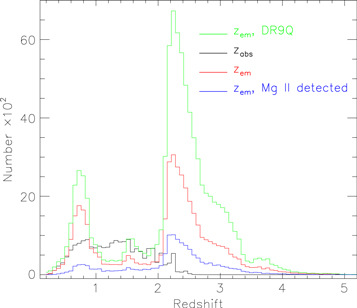
Figure 1. Redshift distributions. The green histogram is for all quasars in the DR9Q sample, the red one represents the quasars used to detect Mg ii absorption, and the blue one represents the quasars with at least one detected Mg ii doublet. The black histogram represents the detected Mg ii absorption doublets.
Download figure:
Standard image High-resolution imageThe criteria used to select the quasar sample and the surveyed spectral region used in our analysis are the following.
- 1.Surveyed spectral region. The spectral region shortwards of the Lyα emission line is dominated by Lyα forest absorption. Thus, in order to avoid the influence of Lyα absorption, we conservatively give up the spectral data shortwards of 1250 Å at quasar rest frame. This leads to quasars with zem > 0.2. The Mg ii absorbers with zabs ∼ zem are likely physically related to the background quasars and can be blueshifted or redshifted by the motion of the absorbing gas clouds within the quasar system (Lü et al. 2007; Vanden Berk et al. 2008; Pan & Chen 2013). The gas clouds must be located in the foreground of the quasar to produce the absorption signature in the quasar spectra. To accommodate the redshift errors and the redshifted absorbers, we restrict ourselves to the spectral data corresponding to a velocity of less than 20,000 km s−1 redward of the quasar Mg ii emission line. Therefore, our spectral region used to search for Mg ii absorption doublets is defined as 1250 × (1 + zem) Å < λ < 2800 × (1 + zem + δz) Å, where δz = zabs − zem = 20,000 km s−1 ×(1 + zem)/c.
- 2.Median signal-to-noise ratio (
 ) per pixel larger than 4. The median value of the of quasar spectra in the surveyed spectral region is ∼4 pixel−1. The cut is set to guarantee robust absorption line measurements.


After taking into account the above limits, we select 43,260 quasars to detect Mg ii absorption doublets. The quasar spectra of the Sloan Digital Sky Survey Data Release 7 (SDSS DR7) have an  of about 8 pixel−1 in the same spectral region as ours, which is higher than our median value of 4 pixel−1. Seyffert et al. (2013) surveyed Mg ii absorption doublets in the SDSS DR7 quasar spectra with an
  of no less than 4 pixel−1, which includes a total of 79,294 quasar spectra. Using the SDSS DR7 quasar spectra, Zhu & Ménard (2013) also completed a systematic survey of Mg ii absorption doublets. The number of quasar spectra used by both Seyffert et al. (2013) and Zhu & Ménard (2013) is about two times the number we use.
The red histogram of Figure 1 shows the emission redshifts of the quasars used to survey the Mg iiabsorption doublets in this work. It is clear that most quasars are located in redshift ranges of 0.4 ≲ zem ≲ 1 and zem > 2. The gas clouds producing Mg ii absorption features in the quasar spectra should be located in the foreground of the quasars, and absorbers might cluster around quasars (e.g., Nestor et al. 2008; Wild et al. 2008; Chen et al. 2015). The wavelength coverage of the Sloan spectrograph is from 3600 to 10400 Å, which defines a redshift range for Mg ii absorption doublets detected from the BOSS quasar spectra from ∼0.27 to ∼2.7 as long as the quasars have higher redshifts. Thus, the distribution of quasar redshifts might affect the distribution of absorber redshifts.
2.2. Spectral Analysis
We closely follow the method described in Chen et al. (2014a, 2014b) to search for Mg ii absorption doublets. Here, we briefly summarize the main steps involved in the detection of absorption lines. We refer readers to Chen et al. (2014a, 2014b) for more details on the method.
In the first step, we fit the underlying continuum plus broad emission lines by invoking a combination of cubic spline and Gaussian functions in an iterative fashion (e.g., pseudo-continuum; Nestor et al. 2005; Quider et al. 2011), which is utilized to normalize the spectral fluxes and flux uncertainties. The upper panel of Figure 2 shows the spectrum of quasar SDSS J121628.03+035031.8 with zem = 0.9966 (black line), overplotted in green is the pseudo-continuum fitting. In the bottom panel, we show the spectrum normalized by the pseudo-continuum fitting in black. The ±1σ and −2σ flux uncertainty levels, which have been normalized by the pseudo-continuum fitting, are also shown with red and blue lines in Figure 2. We eliminate the absorption troughs within the 2σ flux uncertainty level. We disregard the continual absorption features (broad absorption lines; BALs) with widths greater than 2000 km s−1 at depths larger than 10% under the pseudo-continuum.

Figure 2. Example of the pseudo-continuum fitting. Upper panel: the quasar spectrum (black) accompanies the pseudo-continuum fitting (green). Lower panel: the normalized spectrum defined as the quasar spectrum divided by the pseudo-continuum fitting. The red and blue lines are the ±1σ and −2σ flux uncertainty levels, which have also been normalized by the pseudo-continuum fitting.
Download figure:
Standard image High-resolution imageFor the second step, we survey Mg ii doublet candidates with FWHM smaller than 600 km s−1 in the normalized spectra. This routine is mainly dominated by the separations of the Mg iidoublets, which vary with redshift or observed wavelength. We neglect broad or mini-broad absorption features with FWHM > 600 km s−1 as well as weak absorptions within the 2σ flux uncertainty region. We fit a pair of Gaussian functions to model each Mg ii doublet candidate and visually inspect all of the Gaussian fittings one by one. Some strong Mg ii absorption systems might tend toward saturated or self-blended systems. Figure 3 shows an example of strong Mg ii absorption at zabs = 0.4937 imprinted on the quasar spectrum of SDSS J121816.58+364517.4 with a pair of Gaussian function fits, which suggests that a pair of Gaussian functions can also well model the saturated or self-blended Mg ii absorption system.
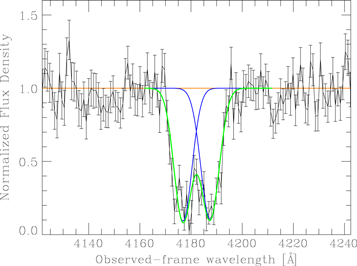
Figure 3. Example of a strong Mg ii absorption doublet at zabs = 0.4937 imprinted on the quasar spectrum of SDSS J121816.58+364517.4. The black lines are the observed data with 1σ uncertainty. The blue lines are a pair of Gaussian function fits and the green is the sum of the blue. At the absorber rest frame, this Mg ii doublet has  ,
,  , FWHMλ2796 = 593 km s−1, and FWHMλ2803 =599 km s−1. The Wr values are obtained by integrating the Gaussian model. This strong system tends toward completely saturated (
 ) and self-blended absorption.See Section 3 for the definition of DR.
Download figure:
Standard image High-resolution imageThe C iv absorption doublets are often detected in the BOSS quasar spectra as well (e.g., Chen et al. 2014a, 2014b). The C iv doublets with high redshifts have velocity separations similar to those of Mg ii doublets with low redshifts. In addition, the absorption strengths and profiles of C iv doublets are parallel to those of Mg ii doublets. These might contaminate the true Mg ii doublets. In order to reduce the confusions of C iv doublets with true Mg ii doublets, we use our previous results for C iv absorption catalogs (Chen et al. 2014a, 2014b) during the individual inspection of the Mg iidoublet candidates.
In the third step, we measure the equivalent widths at the absorber rest frame (Wr) for candidate absorption features by integrating the Gaussian model. The uncertainties on the rest equivalent widths are estimated by
where P(λi − λ0), λi,  , and N are the line profile centered at λ0, the wavelength, the normalized flux uncertainty, and the number of pixels over ±3σ, where σ is given by the best Gaussian fit of the given absorption line candidate. The uncertainty in the pseudo-continuum fitting is not factored into the estimation of the uncertainty of Wr. We estimate the S/Nλ of candidate absorption features (see Qin et al. 2013 for more detail) via

where Sabs is the largest depth within ±3 characteristic Gaussian widths (±3σ) around an absorption feature relative to unity in the normalized spectrum, and σS is calculated by
where Fnoise, Fcont, and N are the flux uncertainty, the flux of the pseudo-continuum, and the number of pixels over ±3 characteristic Gaussian widths (±3σ) around an absorption feature.
Finally, only the absorption doublets with Wr ≥ 0.2 Å and S/Nλ ≥ 2.0 for both the λ2796 and λ2803 lines are retained in our Mg ii absorption doublet catalog.
Among the 43,260 quasars, there are 12,958 with at least one detected Mg ii absorption doublet, whose emission redshifts are shown with the blue solid line in Figure 1. We detect a total of 18,598 Mg ii absorption doublets with 0.2933 ≤ zabs ≤ 2.6529. The distribution of absorption redshifts is shown as the black solid line in Figure 1. We also provide the absorption system properties in Table 1. Previous works (e.g., Nestor et al. 2008; Wild et al. 2008; Chen et al. 2015) noted that absorbers might cluster around quasars. We would like to suggest that the sharp decrease in detected Mg ii doublets at zabs > 2 is due to the poor SDSS spectral quality at λ > 8000 Å since contamination by strong sky spectra.
Table 1. Catalog of Mg ii Absorption Systems
| SDSS NAME | PLATEID | MJD | FIBERID | zem | zabs |

|

|

|

|
S/Nλ2796 | S/Nλ2803 | β |
|---|---|---|---|---|---|---|---|---|---|---|---|---|
| (Å) | (Å) | |||||||||||
| 000009.27 + 020622.0 | 4296 | 55499 | 0616 | 1.4354 | 0.9521 | 1.14 | 8.14 | 0.45 | 3.46 | 7.4 | 3.2 | 0.21767 |
| 000014.07 + 012951.5 | 4296 | 55499 | 0370 | 3.2284 | 1.0077 | 1.52 | 6.91 | 1.27 | 5.52 | 6.4 | 5.2 | 0.63206 |
| 000015.17 + 004833.2 | 4216 | 55477 | 0718 | 3.0277 | 1.5452 | 1.21 | 10.08 | 1.43 | 7.94 | 9.5 | 7.4 | 0.42926 |
| 000016.49 + 022715.1 | 4296 | 55499 | 0642 | 0.8820 | 0.8703 | 1.02 | 6.38 | 0.69 | 4.60 | 5.9 | 4.2 | 0.00624 |
| 000042.90 + 005539.5 | 4216 | 55477 | 0758 | 0.9517 | 0.4965 | 0.52 | 7.43 | 0.46 | 4.60 | 7.1 | 4.4 | 0.25950 |
| 000050.59 + 010959.1 | 4216 | 55477 | 0746 | 2.3678 | 1.9181 | 1.08 | 7.20 | 0.52 | 5.20 | 6.6 | 5.0 | 0.14235 |
| 000050.59 + 010959.1 | 4216 | 55477 | 0746 | 2.3678 | 0.7809 | 0.40 | 5.00 | 0.55 | 4.23 | 4.9 | 4.0 | 0.56295 |
| 000057.58 + 010658.6 | 4216 | 55477 | 0750 | 2.5493 | 0.8182 | 0.78 | 3.12 | 0.92 | 2.56 | 3.0 | 2.4 | 0.58426 |
| 000057.58 + 010658.6 | 4216 | 55477 | 0750 | 2.5493 | 1.0589 | 1.25 | 7.35 | 1.57 | 4.62 | 7.0 | 4.4 | 0.49645 |
| 000104.13 + 010541.6 | 4216 | 55477 | 0788 | 1.9141 | 1.0585 | 1.48 | 5.92 | 1.03 | 6.44 | 5.5 | 5.9 | 0.33423 |
Note. Nσ = Wr/σW represents the significant level of the detection.  .
.
Only a portion of this table is shown here to demonstrate its form and content. A machine-readable version of the full table is available.
Download table as: DataTypeset image
From the SDSS DR7 quasar spectra, Seyffert et al. (2013) found that 26,167 quasars have at least one detected Mg ii absorption doublet, and identified a total number of 35,629 Mg ii absorption doublets. Using about 100,000 quasar spectra from the SDSS DR7 data set, Zhu & Ménard (2013) detected 40,429 Mg ii absorption doublets. These previous two works are larger than ours both in the number of quasars used to survey the Mg ii absorption doublet and the number of resulting doublets.
3. THE MG ii ABSORPTION DOUBLET CATALOG
We characterize the false positives/negatives of detection by calculating the frequency of detected Mg ii absorption doublets (fNALs, see also Chen et al. 2014a, 2014b), which is computed by

where  and
and  represent the numbers of identified Mg ii λ2796 absorption lines and all of the absorption features in the surveyed spectral regions in signal-to-noise ratio bins (
 ). Figure 4 shows the distribution of fNALs with the black solid line, accompanying the distributions of all of the absorption features (red) in the surveyed spectral regions and the detected Mg ii λ2796 absorption lines (blue). fNALs increases with S/Nλ2796 at S/Nλ2796 < and then remains constant at S/Nλ2796 ≥ 4.5. The flat distribution indicates that the detection would likely be complete when S/Nλ2796 > 4.5. In our Mg ii absorption doublet catalog, there are 13,898 doublets with S/Nλ2796 ≥ 4.5. fNALs is a blunt instrument to estimate the detected completeness. Simulating spectra is a good method to address issues of completeness and false positives/negatives. Such simulations are out of the scope of the current work but will be utilized in future works.
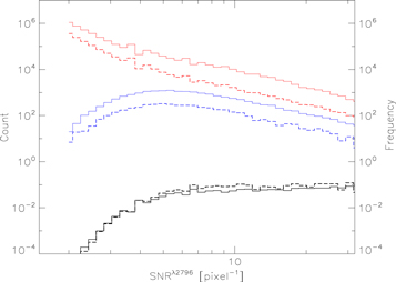
Figure 4. Detected frequency (fNALs) as a function of S/Nλ2796 (black). The solid lines account for all of the Mg iiabsorption doublets, and the dashed lines are for those with zabs > 1.7. The red and blue histograms are for the numbers of all absorption features in the surveyed spectral regions and the identified Mg ii λ2796 absorption lines, respectively. Note a platform in S/Nλ2796 ≳ 4.5.
Download figure:
Standard image High-resolution imageAt S/Nλ2796 < 4.5, we estimate the missing rate (fMR) of several bins of S/Nλ2796 via

where  and fNALs are the average values of fNALs in S/Nλ2796 ≥ 4.5 and the values of fNALs in the corresponding S/Nλ2796 bin, respectively. The derived fMR are provided in Table 2. Generally speaking, the missing rate decreases quickly as S/Nλ2796 increases. fMR is 47% at S/Nλ2796 = 4.5, which suggests a completeness fraction of 53% at S/Nλ2796 = 4.5.
Table 2. The Missing Rate of Absorption Systems with S/Nλ2796 < 4.5
| S/N Bin | [2.0, 2.5] | [2.5, 3.0] | [3.0, 3.5] | [3.5, 4.0] | [4.0, 4.5] | [4.5, 5.0] | [5.0, 6.0] | [6.0, 7.0] |
|---|---|---|---|---|---|---|---|---|
| fMRa | 0.99 | 0.98 | 0.93 | 0.81 | 0.60 | 0.37 | 0.03 | 0.01 |
| fMRb | 0.99 | 0.98 | 0.94 | 0.84 | 0.64 | 0.41 | 0.03 | 0.01 |
Notes.
aThe missing rate for all Mg ii absorption systems. bThe missing rate for Mg ii absorption systems with zabs > 1.7.Download table as: ASCIITypeset image
In order to check the affect of poor sky-line subtraction on our characterization of the false positive/negative detections, we apply the analysis of fNALs and fMR to those Mg ii absorption systems with zabs > 1.7. The results are also shown with the dashed lines in Figure 4 and are provided in Table 2. fMR is 50% at S/Nλ2796 = 4.5, which implies a completeness fraction of 50% at S/Nλ2796 = 4.5. The fNALs and fMR of this subsample parallel those of the whole Mg ii absorption system sample.
Due to the blunt instrument of fNALs, we do not use fMR to correct the number of detected Mg ii absorption doublets in the following analysis.
Figure 5 shows the distributions of Wr. About 25% of absorbers have 0.5 Å  1.0 Å, ∼45% of absorbers have 1.0 Å
  2.0 Å, and ∼25% of absorbers have
  2.0 Å. The ratio of
  (DR) is a valuable indicator of the saturated level of the Mg ii absorption doublet. The theoretical values of DR can vary from 1 for completely saturated absorption to 2 for completely unsaturated absorption (Strömgren 1948). These theoretical limits are also shown by the red solid lines in Figure 5. The middle panel of Figure 5 shows the local data point densities in grayscale, which suggests that the absorption doublets with
  Å tend to be more saturated with increasing
  . We also show the DR distribution in the right panel of Figure 5. The over-plotted blue line is a Gaussian fit. It peaks at DR = 1.13 with σ = 0.245. About 75% of absorbers are located within the theoretical limits of 1 ≤ DR ≤ 2, and about 6% of absorbers lie outside the range of 1 − σ ≤ DR ≤ 2 + σ. We estimate the error of the DR by
About 3.2% of absorbers lie outside the range of 1 − σDR ≤ DR ≤ 2 + σDR. This DR distribution is consistent with previous results (e.g., Quider et al. 2011).
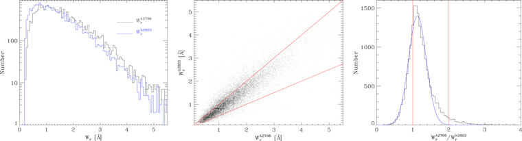
Figure 5. Wr distributions of Mg ii absorption doublets. The red solid lines shown in the middle and right panels represent the theoretical limits of completely saturated ( ) and unsaturated (
 ) absorption, respectively. Middle panel: local data point densities with grayscale. Most of the doublets are saturated with increasing
  . Right panel: the blue line is the Gaussian fitting, which peaks at DR = 1.13 with σ = 0.245.
Download figure:
Standard image High-resolution imageNote that a large fraction (∼25%) of absorbers show DR < 1 or DR > 2, and about 3.2% of absorbers have DR < 1 − σDR or DR > 2 + σDR. In some instances, noise and line blending can lead to the clearly real absorption doublet deviating from the expected value of DR. For example, some absorption doublets can suffer from absorption of other species located at different absorption redshifts. In other instances, false doublets where there are essentially no connection between the two lines can lead to misidentification as Mg ii doublets. Such instances may cause some data to lie outside the theoretical limits of DR.
4. DISCUSSION
4.1. The Incidence Rate of Mg ii Absorbers
The total redshift path covered by our sample as a function of signal-to-noise ratio per pixel (S/Nλ2796) in our surveyed spectral regions is given by
where  if the detection threshold S/Nlim ≤ S/Nλ2796, otherwise gi(S/Nλ2796, z) = 0;
  and
and  are the redshifts corresponding to the maximum and minimum wavelengths in the survey spectral region of quasar i; and the sum is over all of the quasar spectra used to search for Mg ii absorption doublets. Figure 6 shows the total redshift path as a function of S/Nλ2796 or redshift. The conspicuous features of the redshift path at z > 1.5 are probably due to the poor sky-line substraction in the SDSS spectra.

Figure 6. Left panel: redshift path as a function of S/Nλ2796. Right panel: redshift path as a function of redshift. The conspicuous features of redshift path at z > 1.5 are likely due to the poor sky-line substraction in the SDSS spectra.
Download figure:
Standard image High-resolution imageThe incident rate of absorbers is defined as the number of absorbers within an interval of S/Nλ2796 and normalized by the total redshift path, which can be calculated by

where, in the specified redshift bin, Nabs is the number of detected Mg ii absorbers in the given interval of S/Nλ2796 and  is the redshift path of the Mg ii absorber determined by Equation (7). Note that ΔZ(S/Nλ2796) is a function of the S/N of the absorption line, which differs from
  which is a function of the equivalent width of the absorption line (e.g., Seyffert et al. 2013; Zhu & Ménard 2013). Thus, we note the caveat for the incident rate of absorbers that the
  of the current work cannot be compared directly to the same values whose redshift path is determined by the equivalent width of the absorption line (e.g., Seyffert et al. 2013; Zhu & Ménard 2013). We straightforwardly resample the flux of each quasar spectra used to survey the Mg iiabsorption doublets with Monte Carlo simulation from its flux uncertainty constrained by the SDSS to constrain the uncertainty on
  , and then estimate the uncertainty on
  . The
. The  ,
,  , and their uncertainties in different redshift bins are listed in Table 3.
Table 3. The Redshift Number Density
| z bin | Nabs |

|
ΔZ |
|---|---|---|---|
| [0.2933, 0.3933) | 116 |

|

|
| [0.3933, 0.4933) | 350 |

|

|
| [0.4933, 0.5933) | 611 |

|

|
| [0.5933, 0.6933) | 990 |

|

|
| [0.6933, 0.7933) | 1204 |

|

|
| [0.7933, 0.8933) | 1337 |

|

|
| [0.8933, 1.0433) | 1675 |

|

|
| [1.0433, 1.1933) | 1602 |

|

|
| [1.1933, 1.3433) | 1744 |

|

|
| [1.3433, 1.4933) | 1889 |

|

|
| [1.4933, 1.6933) | 2310 |

|

|
| [1.6933, 1.9433) | 2266 |

|

|
| [1.9433, 2.6529] | 2503 |

|

|
Note. Nabs represents the number of the detected Mg ii absorption doublets in corresponding redshift intervals.
Download table as: ASCIITypeset image
In Figure 7, we show the incidence rate of all of the detected Mg ii absorbers as a function of redshift, which increases by about a factor of 6 from z ≈ 0.4 to z ≈ 1.5 and tends to decrease toward higher redshift. Both Seyffert et al. (2013) and Zhu & Ménard (2013) searched for Mg ii absorption doublets in the quasar spectra of the SDSS-I/II, and also found similar redshift evolutions for the incidence rate of Mg ii absorbers with  .
.
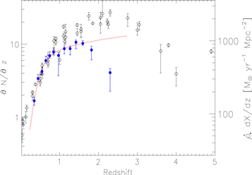
Figure 7. Incidence rate of all the detected Mg ii absorbers (blue filled circles) as a function of redshift. The unfilled diamonds represent the cosmic star formation rate density ( ) scaled by dX/dz, where
  are directly taken from Madau & Dickinson (2014). The red solid line represents the reduced χ2 fitting of Equation (11) to the incidence rate of Mg ii absorbers with zabs < 1.7. The mapping between the left and right y-axes is arbitrary.
Download figure:
Standard image High-resolution imageIn their recent work, Madau & Dickinson (2014) found that the evolution of the star formation rate density follows the parametrization of

where X is the comoving distance, A is the comoving area, and [p1, p2, p3, p4] are fitting parameters. The shape of this evolution scaled by dX/dz can be expressed as
Using FUV and IR data, Madau & Dickinson (2014) found that  increases with redshifts until z ≈ 2 before declining again toward higher redshifts, which is also shown by the unfilled diamonds in Figure 7 after being scaled by dX/dz. Figure 7 shows that both
  and
and  share a parallel evolution at z < 1.7. Therefore, the parametric equation of
  scaled by dX/dz would likely well characterize the incidence rate of Mg ii absorbers. The quickly declining
  at z > 1.7 might be due to an underestimate of the true number of Mg ii absorbers considering the poor sky-line substraction redward of the SDSS spectra. The reduced χ2 fitting of Equation (10) to the incidence rate of Mg ii absorbers at zabs < 1.7 gives [p1, p2, p3, p4] = [0.046 ± 0.053, 12.146 ± 3.974, 12.125 ± 3.642, 1.436 ± 0.061]. The best fit is shown with the red solid line in Figure 7.
[O ii] λ3727 is a good indicator of the star formation rate (Gallagher et al. 1989; Kewley et al. 2004). Thus, the study of [O ii] emission and Mg ii absorption might provide a clue toward the relationship between star formation within galaxies and the properties of Mg ii absorbers. In fact, a number of previous studies have suggested a relationship between strong (Wr ≳ 1 Å) absorbers and star formation. Using more than 8500 strong (Wr > 0.7 Å) Mg ii absorbers measured from the SDSS quasar spectra, Ménard et al. (2011) detected a tight correlation between  and mean [O ii] luminosity density, which can be reproduced by a Monte Carlo simulation (López & Chen 2012). Based on a sample of intermediate-redshift star-forming galaxies, Noterdaeme et al. (2010) found that the stronger (Wr > 1 Å) Mg ii absorbers, which were detected from the quasar spectra, match the higher average luminosities of the [O ii] emission measured from the foreground galaxy spectra. No matter what the absorption strengths are, Shen & Ménard (2012) found that the composite quasar spectra with Mg ii associated absorption doublets (zem ≈ zabs) exhibit a significant excess in [O ii] emission when compared to the unabsorbed quasars. The dependence of strong Mg ii absorbers on [O ii] emission implies that the Mg ii absorbers can trace the cosmic star formation history. In our catalog, about 75% of Mg iiabsorbers have
  . The parallel redshift evolutions of the star formation rate density and the incidence rate of Mg ii absorbers (see also Matejek & Simcoe 2012; Seyffert et al. 2013; Zhu & Ménard 2013) suggest a valuable clue to investigate the cosmic star formation history through strong absorbers.
We note a caveat in the connection between the absorber and the star formation history. Not all Mg ii absorbers form within star-forming galaxies (e.g., Zibetti et al. 2007; Gauthier & Chen 2011). For weak absorbers (Wr < 1 Å), the colors of galaxies do not obviously correlate with the absorption strength (e.g., Chen et al. 2010a; Kacprzak et al. 2011b), which implies the lack of a strong relationship between the absorption strength and the recent star formation rate within the galaxies. The redshift number density evolution of the weak absorbers shows no or only weak evolution (e.g., Nestor et al. 2005; Matejek & Simcoe 2012). The difference in redshift number density evolution between weak absorbers and strong absorbers suggests that there may be different origins for weak and strong absorbers.
4.2. The Quasar-frame Velocity Distribution
Using large quasar absorber samples, several previous studies (e.g., Nestor et al. 2008; Wild et al. 2008; Chen et al. 2015) suggest that absorbers with zabs ≈ zem would likely cluster around quasars. However, there is a common feature in their studies that β shows an asymmetrical distribution around β ≈ 0, which might be caused by outflows; β is defined as follows:
The derivation of β is given in the

Figure 8. Relative velocity distribution of all Mg ii absorbers in our Mg ii absorption doublet catalog. The insert figure is the zoom in region with −0.01 < β < 0.04. A distinct excess of Mg ii absorbers at β ≈ 0 ∼ 0.02 is obvious.
Download figure:
Standard image High-resolution imageAccurate emission redshifts of quasars are crucial for the shape of the β distribution, especially for those absorbers with zabs ≈ zem. Large errors will be introduced to redshifts estimated from broad emission lines compared to those estimated from host galaxy absorption lines or narrow emission lines (e.g., [O iii] λ5007; Hewett & Wild 2010). We construct a lower-redshift quasar sample by cutting our Mg ii absorption catalog to those quasars with zem ≤ 1.0770, for which the emission line redshift can be determined from the narrow emission lines.
The quasar subsample with zem ≤ 1.0770 contains a total number of 1677 Mg ii absorption doublets, whose β distribution is shown in Figure 9. Note that distinct excess of Mg ii absorbers at β ≈ 0 ∼ 0.02 and the approximately flat distribution in β ≳ 0.03. Our Mg ii absorption catalog probably includes all three kinds of absorbers: (1) cosmologically intervening absorbers; (2) environmental absorbers (associated absorbers) that reside within quasar host galaxies or galaxy clusters/groups; and (3) intrinsic absorbers that are physically related to the quasar central region. We statistically identify the three kinds of absorbers as follows.
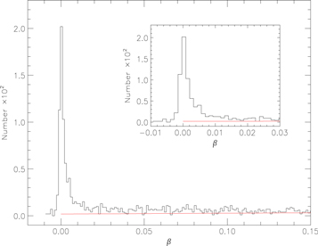
Figure 9. Relative velocity distribution for Mg ii absorbers with zem ≤ 1.0770. The insert figure is the zoom in region with −0.01 < β < 0.03. Note the distinct excess of Mg ii absorbers at β ≈ 0 ∼ 0.02 and the approximately stable distribution in β ≳ 0.03. The red solid line represents the linear-fit to the data with 0.05 < β < 0.15, which is extrapolated to all data with β > 0.
Download figure:
Standard image High-resolution image(1) Cosmologically intervening absorbers. The smooth tail of the β distribution suggests that the Mg ii absorption doublets with β ≳ 0.03 would probably be dominated by cosmologically intervening absorption. We adopt a linear function to fit the data with 0.05 < β < 0.15, which gives Number = (1.876 ± 0.896) + (8.812 ± 8.710) × β. We extrapolate the linear-fit to all of the data with β > 0 to characterize the contribution of the cosmologically intervening absorbers, which is shown with the red solid line in Figure 9. This linear fit accounts for a total of 1100 Mg ii absorbers with β > 0, namely, 1100 cosmologically intervening Mg ii absorbers.
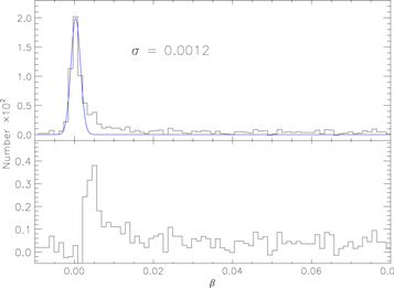
(2) Environmental absorbers. The β distribution of Mg ii absorbers subtracted off the extrapolated linear-fit is shown in the top panel of Figure 10. We assume a Gaussian component centered at β = 0 to fit the data with β < 0, which gives σ = 0.0012. The Gaussian fit is extrapolated to the data with β > 0, which is shown with the blue solid line in the top panel of Figure 10. We adopt the extrapolated Gaussian fit to trace the environmental absorbers, which accounts for a total of 500 Mg ii absorbers, namely, 500 environmental absorbers.
Figure 10. Relative velocity distributions as those shown in Figure 9. Top panel: the data have been taken from the contribution of the cosmologically intervening absorbers. The blue solid line represents the Gaussian fit centered at β = 0 to the data with β < 0, which give a σ = 0.0012. Bottom panel: the data have been taken from the contributions of both the intervening and environmental absorptions. Note the remarkable peak at β ≈ 0.005.
Download figure:
Standard image High-resolution image
(3) Intrinsic absorbers. The β distribution of the Mg iiabsorbers subtracted from the combination of the extrapolated linear-fit and the extrapolated Gaussian fit is shown in the bottom panel of Figure 10, which contains 77 Mg ii absorbers. The significant excess of the β distribution in 0.00 ≲ β ≲ 0.02 is very interesting because it likely represents the contribution from quasar outflows. This excess peaks at υ ≈ 1500 km s−1 and shows an asymmetric distribution. Here, some caveats cannot be ignored. The extrapolated Gaussian fit might overestimate environmental absorbers with low-relative velocities. In addition, the extrapolated linear fit might overestimate cosmologically intervening absorbers with low relative velocities. These overestimates may partly contribute to the rapid decrease of the quasar outflow component at low velocities. Nestor et al. (2008) and Chen et al. (2015) found that the similarly asymmetric distribution of β also exists for C iv absorbers, which peaks at v ≈ 2000 km s−1. The ionization potentials are 15.035 eV for Mg ii and 64.49 eV for C iv. These different peak velocities imply that higher ionization intrinsic absorbers might be formed in higher velocity outflows. However, we note that the quasar emission redshifts where the C ivabsorber is detected are mainly estimated from broad emission lines, which might introduce large errors to the β of the C iv absorbers.
5. SUMMARY
We have conducted a systematic survey for Mg ii λλ2796, 2803 absorption doublets in the BOSS quasar spectra (DR9Q) with median  per pixel. Our analysis is limited to the spectral data between 1250 Å (rest frame) and the red wing of the Mg ii λ2800 emission line of the quasar. The Mg ii absorption catalog only has doublets with Wr ≥ 0.2 Å and with absorption line signal-to-noise ratio S/Nλ ≥ 2.0, which includes a total of 18,598 doublets with 0.2933 ≤ zabs ≤ 2.6529. About 95% of absorbers have
  , about 75% of absorbers have
  , and a large fraction (∼25%) have
  . Most absorbers (75%) fall into the theoretical limits of completely saturated absorption and completely unsaturated absorption (1 ≤ DR ≤ 2), and about 3.2% of absorbers lie outside the range of DR < 1 − σDR or DR > 2 + σDR, where σDR is the error of the doublet ratio DR.
We compute the frequency of detected Mg ii absorption doublets (fNALs) to trace the completeness of the detection, which suggests that our detection would likely be complete when S/Nλ2796 is greater than 4.5. There are 13,898 doublets with S/Nλ2796 ≥ 4.5 in our Mg ii absorption doublet catalog.
The incidence rate of Mg ii absorbers ( ) shows a moderate evolution, increasing by about a factor of 6 until z ≈ 1.5. This trend parallels the evolution of the cosmic star formation rate density (
 ). The similar pattern of evolution implies that the Mg ii absorber might be used as a probe of the cosmic star formation history within galaxies.
We reduce our Mg ii absorption catalog to those quasars with zem ≤ 1.0770 so that the narrow emission line of [O iii] λ5007 can be available in the BOSS quasar spectra, resulting in a total of 1677 Mg ii absorption doublets. The relative velocities (β) of the Mg iiabsorbers in this subsample show a complex distribution; that is, a significant excess at β ≈ 0, a smooth tail at β ≳ 0.03, and a distinct excess at β ≈ 0 ∼ 0.02. This complex β distribution indicates that our Mg ii absorption catalog likely includes three classes of absorbers: (1) cosmologically intervening absorbers; (2) environmental absorbers that are located within the quasar host galaxies or galaxy clusters; and (3) quasar outflow absorbers. We adopt an extrapolated linear fit to all of the absorbers with β > 0 to trace the cosmologically intervening absorbers, and a Gaussian component located at β = 0 to model the environmental absorbers. The β distribution subtracted from the extrapolated linear fit and the Gaussian component might mainly consist of the quasar outflow absorbers, which peaks at υ ≈ 1500 km s−1 and rapidly decreases at lower velocities. This peak velocity is lower than the value of 2000 km s−1 reached by the statistical analysis of C iv absorbers.
We sincerely thank the anonymous referee for very helpful comments and structural suggestions. We acknowledge professor Yi-Ping Qin (Guangzhou University, China) for helpful conversations. This work was supported by the National Natural Science Foundation of China (NO. 11363001, grants 11273015 and 11133001), National Basic Research Program (973 program No. 2013CB834905), the Guangxi Natural Science Foundation (2015GXNSFBA139004), and the Guangxi University of Science and Technology research projects (No. KY2015YB289).
Funding for SDSS-III has been provided by the Alfred P. Sloan Foundation, the Participating Institutions, the National Science Foundation, and the U.S. Department of Energy Office of Science. The SDSS-III web site is http://www.sdss3.org/.
SDSS-III is managed by the Astrophysical Research Consortium for the Participating Institutions of the SDSS-III Collaboration including the University of Arizona, the Brazilian Participation Group, Brookhaven National Laboratory, Carnegie Mellon University, University of Florida, the French Participation Group, the German Participation Group, Harvard University, the Instituto de Astrofisica de Canarias, the Michigan State/Notre Dame/JINA Participation Group, Johns Hopkins University, Lawrence Berkeley National Laboratory, Max Planck Institute for Astrophysics, Max Planck Institute for Extraterrestrial Physics, New Mexico State University, New York University, Ohio State University, Pennsylvania State University, University of Portsmouth, Princeton University, the Spanish Participation Group, University of Tokyo, University of Utah, Vanderbilt University, University of Virginia, University of Washington, and Yale University.
APPENDIXDOPPLER RELATIVE VELOCITY
According to the theory of special relativity, an absorber moving toward the observer at a velocity of υ in the quasar rest frame produces a Doppler redshift of
where β ≡ υ/c and c is the speed of light. Thus, we have
Assuming that the absorber is intrinsic to or physically associated with the quasar, the difference in emission redshift and the absorption redshift, measured from the same quasar spectrum, would originate from the Doppler motion of the absorber with respect to the quasar. The Doppler redshift can be estimated by the emission redshift and the absorption redshift (see, e.g., Lü et al. 2007):

The positive zDopp suggests that the absorber is moving away from the quasar, while the negative zDopp reflects the fact that the absorber is moving toward the quasar. Combining Equations (13) and (14), we have

When the value of zDopp is small, one can obtain the following from Equation (13) by performing a Taylor expansion and retaining the terms of zDopp to second order:

Note that since both β and zDopp are dimensionless quantities, the square of zDopp does not violate this equation. Ignoring the second-order term in Equation (16) gives rise to

which is a well-known equation between the Doppler velocity and the Doppler redshift (note that this equation will be valid when the Doppler redshift is very small).
Applying Equation (14) to (17), one gets

In this paper, we use Equation (15) instead of Equation (18) to estimate β, in case some of the absorbers move quite fast.