


ABSTRACT
We present ∼47,000 periodic variables found during the analysis of 5.4 million variable star candidates within a 20,000 deg2 region covered by the Catalina Surveys Data Release-1 (CSDR1). Combining these variables with type ab RR Lyrae from our previous work, we produce an online catalog containing periods, amplitudes, and classifications for ∼61,000 periodic variables. By cross-matching these variables with those from prior surveys, we find that >90% of the ∼8000 known periodic variables in the survey region are recovered. For these sources, we find excellent agreement between our catalog and prior values of luminosity, period, and amplitude as well as classification. We investigate the rate of confusion between objects classified as contact binaries and type c RR Lyrae (RRc's) based on periods, colors, amplitudes, metallicities, radial velocities, and surface gravities. We find that no more than a few percent of the variables in these classes are misidentified. By deriving distances for this clean sample of ∼5500 RRc's, we trace the path of the Sagittarius tidal streams within the Galactic halo. Selecting 146 outer-halo RRc's with SDSS radial velocities, we confirm the presence of a coherent halo structure that is inconsistent with current N-body simulations of the Sagittarius tidal stream. We also find numerous long-period variables that are very likely associated within the Sagittarius tidal stream system. Based on the examination of 31,000 contact binary light curves we find evidence for two subgroups exhibiting irregular light curves. One subgroup presents significant variations in mean brightness that are likely due to chromospheric activity. The other subgroup shows stable modulations over more than a thousand days and thereby provides evidence that the O'Connell effect is not due to stellar spots.
Export citation and abstract BibTeX RIS
1. INTRODUCTION
The 1638 discovery of the periodic variability of Mira by Holwarda (Hoffleit 1997), was the beginning of a new age of understanding in astronomy. Periodic variables, such as Cepheids and RR Lyrae, underpin the cosmological distance scale (Freedman et al. 2001) while also providing insight into the processes and properties of galaxy formation (Saha 1984, 1985; Catelan 2009). On smaller scales, the periodic motions and interactions of binaries provide insight into stellar evolution and multiplicity. Under the right circumstances, such pairs can also provide estimates of stellar masses, sizes, densities, shapes, and orbits (e.g., Southworth 2012 and references therein).
By the early 1980s, many thousands of variable stars were known (Roth 1994). However, it was not until the 1990s that microlensing surveys changed the scale of variable star research. Groups such as MACHO (Alcock et al. 1993) and OGLE (Udalski et al. 1994) began to regularly deliver a treasure trove of tens of thousands of periodic variable stars in the Magellanic Clouds and Galactic center (e.g., Alcock et al. 1996, 1997, 1998, 1999, 2000a, 2000b, 2001, 2002; Mateo et al. 1995; Udalski et al. 1996, 1998, 1999; Szymanski et al. 2001; Wozniak et al. 2002). These surveys remain the major source of the more than 200,000 periodic variables that are currently known.
Over much larger and less crowded areas of the sky, the very wide field cameras of the ASAS survey (Pojmanski 1997) soon led to the discovery of tens of thousands of variable stars down to V = 13 (Pojmanski 2000, 2002, 2003; Pojmanski & Maciejewski 2004a, 2004b; Pojmanski et al. 2005). Similar work was also undertaken using data from the Robotic Optical Transient Search Experiment (ROTSE; Akerlof et al. 2000) as part of the Northern Sky Variability Survey (NSVS; Wozniak et al. 2004; Kinemuchi et al. 2006; Hoffman et al. 2009). Surveys for planetary transits have also discovered periodic variable stars (e.g., HATNet, Hartman et al. 2011; BOKS, Feldmeier et al. 2011).
More recently, researchers have been motivated to study the variable star populations spanning the sky to much greater depths. This has led to the harvest of variable stars from archival data taken by near-Earth object (NEO) surveys. Data from the Lowell Observatory Near-Earth Object Search (LONEOS; Bowell et al. 1995) has been searched by Miceli et al. (2008), while data from the Lincoln Near-Earth Asteroid Research (LINEAR; Stokes et al. 2000) was analyzed by Sesar et al. (2013) and Palaversa et al. (2013). Similarly, in our preliminary work (Drake et al. 2013a, 2013b) we harvested type ab RR Lyrae variables from the Catalina Sky Survey (Larson et al. 2003) photometry presented in CSDR1 (Drake et al. 2012). In this paper, we will further investigate CSDR1 photometry in order to complete our search for periodic variable stars.
2. OBSERVATIONS
The Catalina Sky Survey10 began in 2004 and uses three telescopes to cover the sky between declination δ = −75° and +65° in order to discover near-Earth objects (NEOs) and potential hazardous asteroids (PHAs). Each of the survey telescopes is run as a separate subsurveys. These consist of the Catalina Schmidt Survey (CSS) and the Mount Lemmon Survey (MLS) in Tucson, AZ, and the Siding Spring Survey (SSS) in Siding Spring, Australia. Each telescope has set fields that tile the sky and avoid the Galactic plane region by 10°–15° due to reduced source recovery in crowded stellar regions. All images are taken unfiltered to maximize throughput. The observations analyzed in this work were taken in sets of four images separated by 10 minutes with typical exposure times of 30 s. Photometry is carried out using the aperture photometry program SExtractor (Bertin & Arnouts 1996). In addition to asteroids, all the Catalina data is analyzed for transient sources by the Catalina Real-time Transient Survey (CRTS;11 Drake et al. 2009; Djorgovski et al. 2011).
In this paper, we concentrate on the data taken by the CSS 0.7m telescope between 2005 April and 2011 June, that was made publicly available via CSDR1 (Drake et al. 2012) in 2012 January. Individual detections in CSDR1 are matched with sources from a deeper "master" catalog derived from the median co-addition of 20 or more images. The CSDR1 data set has an average of 250 observations per field. Each CSS image covers 8.2 deg2 on the sky. In total, the CSDR1 includes 198 million discrete sources with 12 < V < 20 (Drake et al. 2013a). We have chosen to select only the 20,155 deg2 covered by CSDR1 in the region 0° < α < 360° and −22° < δ < 65° as sources below δ = −22° have better temporal coverage in SSS data that became available in 2013 January as part of Catalina Surveys Data Release 2 (CSDR2)12 and will be analyzed separately.
3. VARIABLE SOURCE SELECTION
In order to find the variable sources with CSDR1 we began by selecting variables based on values of the Stetson variability index (JWS; Stetson 1996) using the weighting scheme of Zhang et al. (2003). The current analysis method follows Drake et al. (2013a, 2013b). However, we have revised our variable selection process to better account for blending, which occurs in CSDR1 photometry as it is based on SExtractor aperture magnitudes. During poor seeing or sky conditions, close pairs or groups of sources are detected as a single object, while in good seeing conditions the objects are resolved and appear at their true brightness. Blending is important for variable star selection since variations in seeing cause artificial changes in the apparent brightness of many catalog objects.
Candidate blended sources can be found by selecting master catalog objects that have multiple detections from a single observation. However, these multi-detection associations can also occur due to image artifacts and transient sources (such as passing asteroids). Thus, even isolated objects often have some nights where multiple detections have been matched from a single image.
To reduce the effect of blends we investigated the distribution of the number of detections (Nobs) for a few of the observation fields. Sources in the range 14 < VCSS < 17 are not affected by saturation or the natural decline in detection efficiency with decreasing brightness. Using these sources, we determined the average number of detections for sources within a field (Navf). By inspecting the light curves of the objects with high numbers of detections, we found that objects with Nobs > 1.07Navf were usually significantly affected by a neighboring source. We removed all variable candidates with VCSS > 14 that had more detections than this threshold.
In contrast to additional detections due to blending, sources with VCSS < 14 often have Nobs well below Navf. This is because of saturation since such observations were flagged and removed from our period search. This means that the brightness sources may have few good observations. Nevertheless, we found that it was possible to detect variability for sources brighter than V = 12 because such sources are not saturated in poor seeing or when they have dimmed significantly. Therefore, to reduce the presence of artificial variability due to saturation effects, we only remove objects with V < 14 that have Nobs < 0.3 × Navf. Nevertheless, it is prudent to be cautious about the small fraction of sources near the saturation limit. The data from shallower surveys, such as ASAS (Pojmanski 1997) and NSVS (Wozniak et al. 2004), may be used to further verify the nature of these sources.
In addition to the change to our treatment of blended and saturated sources, we discovered that there were systematic variations in the photometric noise level between fields. Therefore, instead of adopting a universal JWS variability threshold as per Drake et al. (2013a), we derived separate thresholds for each field.
First, we ordered all the sources within each field by their average magnitude. We then determined the average variability ( ) and its standard deviation (σJ) in groups of 200 sources. Since highly variable sources bias the JWS distribution, we perform a 3σ clipping on the values and redetermine the average and sigma values of this statistic. As there are thousands of sources in each field with VCSS > 16, we combined JWS values in 0.25 mag bins to provide more robust values. Variable candidates were selected at a 3.5σJ threshold that was interpolated to their observed average brightness.
In Figure 1, we plot the magnitude distribution of JWS values for the sources in two fields as well as with the variability threshold used by Drake et al. (2013a). This plot demonstrates that there is a significant variation in the distribution of JWS values with source brightness and field. In contrast to Drake et al. (2013a), where 8 million variable candidates were selected, our new selection reduces this number to 5.4 million. This is 2.7% of the total number of catalog sources.

Figure 1. Distribution of Stetson JWS variability index for two fields analyzed in this work. The variable candidates are plotted as large green dots. The dashed line shows the selection used by Drake et al. (2013). The solid red line shows the new variability threshold calculated on a brightness and field-by-field basis. In the left panel, we plot sources for CSS field S01004 (centered at  , δ = −01°24'40
 00). In the right panel, we plot objects in CSS field N12065 (centered at
  , δ = +12°41'5989).
Download figure:
Standard image High-resolution image4. SELECTION OF PERIODIC VARIABLES
We ran a Lomb–Scargle (LS; Lomb 1976; Scargle 1982) periodogram analysis on all the variable candidates. Candidate periodic variables were selected based on an LS significance statistic of η < 10−5. One hundred fifty-four thousand candidates were found in addition to the ∼15,000 known CSS RRab's (Drake et al. (2013a, 2013b). This threshold matches that used by Drake et al. (2013b) since ∼15% of RRab's in the CSS data were found to have been missed because of the higher (η < 10−7) threshold used by Drake et al. (2013a).
Although our variability selection process noted above removes bright blends, faint stars have fewer detections because of lower detection efficiency. To remove blends among faint sources, we select objects with <5% coincident detections from the individual images. This reduces the number of periodic candidates to 144,000 sources. We allow small numbers of multi-detections since, apart from multiple detection due to artifacts, some faint neighboring objects may only appear in good seeing. Such objects only have a minor effect on the overall photometry and period determination.
As with Drake et al. (2013a, 2013b), the Adaptive Fourier Decomposition (AFD) method (Torrealba et al. 2014) was run on all candidates to determine the best period for each source. As expected, there are many cases where a false signal is found due to the sampling pattern as well as variation in lunar phase and location. These effects lead to period estimates that are near-fractions and multiples of a sidereal day, as well as near-sidereal and synodic months. We investigated the extent of each of these aliases and removed candidates lying within the range of each period alias. There is also significant evidence for seasonal and annual variations. As these features are broad, they were not removed. However, as we will show, these sources are removed during inspection. The removal of aliases reduces the numbers of candidates to 128,000. We expect that a small fraction (a few percent) of true variables with periods within these ranges were also removed by these cuts.
A clear way to reduce the number of nonperiodic objects along the candidates is to select sources based on the goodness-of-fit or reduced χ2 ( ) of the best AFD period. As expected, we found that most of the periodic variable candidates had
  . A poor fit generally signifies either that an object is not periodic or the best fit period is incorrect. However, sources such as long-period variables (LPVs) exhibit significant periodicity, yet are poorly fit by a low-order (⩽6) Fourier series due to moderately large variations in amplitude over time. To simultaneously retain the significantly periodic sources while removing poorly fit aperiodic sources, we removed the candidates that had both
  and η < 10−9. The resulting set contains ∼112, 000 candidates.
In Figure 2 we compare the period–amplitude distribution of the initial 154,000 periodic candidates with the ∼112, 000 sources remaining after removing blends, period alias, and sources with poor AFD fits.

Figure 2. Period–amplitude distribution of candidate variables. In the top plot we show the period distribution before removing the objects with Fourier fits with  or periods due to sampling aliases.
Download figure:
Standard image High-resolution imageAll 112, 000 periodic candidates were inspected (by A.J.D.) using a custom-built Web service. This process involved classifying the variable types as well as flagging objects that had periods that were slightly incorrect or completely incorrect but still probably periodic variables. The classification process itself mainly involved examination and comparison of the phased (and in some cases unphased) light curve morphology with known types of periodic variables. To improve this process, additional consideration was always given to the range of periods, amplitudes, and colors that different types of variables are known to have. For example, short-period contact binaries are generally red, while RR Lyrae are blue. The values of the M test statistic (described below) were also considered. However, none of these individual parameters was specifically used to classify or exclude types of variable since the observational data themselves contain some objects with unusual values, for example, unexpected colors due to blending that could be confirmed when examining higher resolution SDSS images.
In ambiguous cases, such as may arise for faint objects, or when multiple types of variability are present, the most evident and likely individual types based on the combined information cases where the presence of actual periodicity was in question were vetoed. Due to the nature of the process, it is highly likely that some observational biases exist. It is also possible that some objects have best fit periods that are aliases of their true period. This could lead to the type of variability being wrongly classified.
During the inspection process, the initial periods of a large number of the sources were improved and corrected. In particular, most of the contact binaries were initially found at half of their true period because of the symmetry of their light curves. This half-period effect is a well-known problem (e.g., Richards et al. 2012). Additionally, in ∼2500 cases, the AFD periods were very close to correct, but clearly not correct. We improved the period determinations of these sources interactively by making very slight adjustments to the period. As the actual final changes are generally ≪0.01%, the process almost always converged very quickly. However, in the case of detached eclipsing binaries, we often found the correct period by investigating the harmonic frequencies.
In total, ∼47, 000 light curves were classified as corresponding to periodic variables. Of these, 396 are objects with multiple light curves due to overlap between fields. The duplicates include 45 RRab's previously given by Drake et al. (2013a, 2013b). The number of unique periodic variables is 46, 668. Another 4800 objects remain periodic candidates and will be provided online.13 In Table 1, we show the effect of selections on the total number of candidates.
Table 1. Periodic Variable Selection
| Selection | Objects |
|---|---|
| CSS Sources | 198 million |
| Variable Cand. | 5.4 million |
| LS η < 10−5 | ∼154000 |
| Nblend < 5% | ∼144000 |
| P ≠ Palias | ∼128000 |
 or η < 10−9 or η < 10−9 |
∼112000 |
| Periodic | 46668 |
Notes. Column 1: selection used to select the sample of objects. Column 2: number of objects following the subselection. These numbers do not include the ∼14, 000 known RRab's from Drake et al. (2013a, 2013b).
Download table as: ASCIITypeset image
5. GENERAL PROPERTIES OF THE PERIODIC VARIABLES
To see how the visually selected periodic variables differ from the initial candidates, we investigated the period, amplitude, and magnitude properties of the sources. In Figure 3, we plot the period–amplitude distribution of the periodic variables in the catalog. In contrast to Figure 2, here we plot the final periods of the objects rather than their initial periods. Very few objects remain at periods less than 0.2 days. These objects are contact binaries suffering from the half-period effect, as noted above. Additionally, very few objects with periods longer than 10 days remain. In particular, there are no sources with periods longer than 1000 days. Most of the stars with long periods are LPVs. There are very few LPVs in the fields we observed away from the Galactic disk. The foreground LPVs are generally undetectable since they are bright and thus saturated within the images. Some stars are known to have longer periods. However, like LPVs, such stars are generally near our saturation limit. Additionally, the length of our data does not provide strong constraints for objects with very long periods. Most of the candidates that were found at very long periods had best-fit periods matching the time span of the data. Many of these sources were found to be quasars (QSOs) and were clearly not periodic.

Figure 3. Period–amplitude distribution of the periodic sources selected after inspection of light curves.
Download figure:
Standard image High-resolution imageA comparison of the periods for the 396 objects with multiple light curves revealed ∼10 of the objects had different periods. Inspection of the light curves revealed that almost all of these cases were due to contact binaries that were also well fit when folded at an alias of their true periods. Since contact binaries dominate the number of periodic variables in this catalog, we expect that ∼10% of the periods presented here are aliases.
In Figure 4, we present the distribution of LS periodic significance (η) for the catalog variables. This plot shows us that <10% of the periodic candidates with η = 1 × 10⁻⁶ were found to be periodic. However, since a very large fraction of the sources were found at this level, they constitute >7% of the total number in the catalog. This result suggests that a large number of periodic sources remain to be found at low levels of significance. However, since there are millions of sources at this level, their discovery within these data requires either new techniques or automated methods of classification and verification. The number of aperiodic variables within these data (such as QSOs) far outnumbers the periodic sources (M. J. Graham et al. 2014, in preparation).

Figure 4. Fraction of periodic objects compared with LS significance. In the top panel we plot the fraction of the 112, 000 initial periodic variable candidates (FIP) that made it into our catalog. In the lower panel we plot the fraction of all periodic catalog sources (FAP) found each LS significance level.
Download figure:
Standard image High-resolution imageIn Figure 5, we present the distribution of AFD fit  values for the initial periodic candidates and the final catalog sources. As expected, these figures show that most of the remaining periodic sources are moderately good fits with
  . Most of the faint sources with large
  values have been removed. However, many of the sources with VCSS < 13, where saturation increases the value of
  , were found to be periodic. In addition, we see that most of the remaining sources in the range 14 < VCSS < 18 have
  values significantly less than one. Low values of
  can be caused by fitting too many parameters to the data or inaccurate estimates of uncertainty. In this case, these low values are due to the systematic overestimation of the CSDR1 error-bars. For the brightest sources, the average
  is approximately 0.3, suggesting that the actual photometric uncertainties are ∼0.5 the CSDR1 values. The fact that the CSDR1 errors are overestimated was demonstrated by Palaversa et al. (2013). They compared CSDR2 light curves with those from LINEAR. They found that the Catalina error bars were larger, yet the objects phased with the correct periods generally show less scatter. This is also demonstrated by the low average values of JWS. The overestimated photometric uncertainties do not affect the results in this analysis.

Figure 5. Fourier-fit  values for periodic variable candidates. In the left panel we plot the distribution for the 128,000 periodic candidates before imposing the
  selection. In the right panel we plot the distribution for the periodic sources in the final catalog.
Download figure:
Standard image High-resolution imageIn Figure 6, we compare the distribution of mean magnitudes for the initial periodic variable candidates with the final catalog variables. The largest number of periodic sources are found near V = 16. This result is in contrast to the peak of the RRab magnitude distribution from Drake et al. (2013a), which occurred at V = 17. To demonstrate the reason for this difference, we separate the main types of periodic variables and plot them in Figure 7. Here we see that the contact eclipsing binaries dominate the number of periodic variables, and on average, they are brighter than the RR Lyrae. Unlike the RR Lyrae, eclipsing binaries are mostly main-sequence stars with spectroscopic types earlier than M (Norton et al. 2011). These systems generally lie within the Galactic disk. Hence, since CSS observations are concentrated away from the disk, only foreground eclipsing binaries are detected. Figure 7 also presents the period distributions for the main types of periodic variables detected. It is evident that Drake et al. (2013a) missed a small number of RRab's that have periods similar to RRc's and RRd's.

Figure 6. Distribution of average CSS magnitudes. The red dashed line shows the magnitude distribution of variables candidates before inspection. The blue solid line shows the distribution for objects in the periodic variable catalog.
Download figure:
Standard image High-resolution image
Figure 7. Distribution of the main types of periodic stars. In the left panel we plot the magnitude distribution and in the right we plot the period distribution. The solid green line presents the eclipsing binaries. The short-dashed blue line presents RRc's. The dot-dashed red line presents RRab's from this analysis, while for comparison, the dotted black line gives RRab's from Drake et al. (2013a, 2013b).
Download figure:
Standard image High-resolution image6. TYPES OF VARIABLES
Each of the periodic variables found among the candidates were classified into three broad classes: eclipsing, pulsating and rotational. The pulsational objects can be divided into δ Scutis, RR Lyrae, Mira and semi-regular variables, and Cepheids. Among these we further divide the δ Scutis into those with amplitudes V > 0.1 (high-amplitude δ Scutis, HADS), and those with V < 0.1 (low-amplitude δ Scutis, LADS) based on Alcock et al. (2000c). The RR Lyrae class consists of RRab's (fundamental mode), RRc's (first overtone mode), RRd's (multi-mode) and Blazkho (long-term modulation; Blazkho 1907) types. The Cepheid class includes classical (type I) Cepheids, type II Cepheids (Cep-II), and anomalous Cepheids (ACEPs). However, we did not find any clear classical Cepheids. We include both semi-regular variables and Mira variables under a single, LPV classification.
The eclipsing variables in our data were generally divided into a contact and semi-detached binary (EW/EB) group and detached systems (EA) following Palaversa et al. (2013). However, during a review of all the EA's we further divided these systems into semi-detached β Lyrae (EB) systems and true Algol (EA) variables. Our EB group is thus incomplete, with those systems that closely resemble contact systems being placed in the original EW/EB group. We found a number of EA variables where it was not possible to determine the period due to an insufficient number of eclipses. These objects were placed in an unknown-period (EAUP) class. We also discovered many eclipsing white dwarf and subdwarf binary systems. These are included in a post-common-envelope (PCEB) class. A small group of periodic variables exhibiting distorted light curves and varying minima and maxima was discovered. As the nature of these sources is unclear we place them in the "hump" variable class (see Section 6.9).
The variable stars that we discovered from the rotating variable class include ellipsoid variables (ELL) and spotted (RS CVn) systems. Our inspection also led us to retain 4808 systems in a periodic candidates class (PCANDs). The light curves of these objects appeared to exhibit regular variations, yet their best-fit periods were clearly incorrect. Since it is uncertain whether these objects are truly periodic sources, they are not included in the catalog. Based on the results of Graham et al. (2013), it was expected that there would be some variables where the correct period could not be found, even though we applied multiple search techniques.
In Figure 8, we plot the sky distribution for each of the classes of periodic variables having more than 100 members. As expected, the eclipsing binaries are concentrated at low Galactic latitudes, while the halo stars, such as RR Lyrae, are much more uniformly distributed.

Figure 8. Distribution of types of periodic variables in the CSS catalog. In panel (1) we plot the distribution of rotational variables (blue) and δ Scutis (red). In panel (2) we plot LPV's (red) and Cepheid variables (blue). In panel (3) we plot contact eclipsing binaries (blue) and detached binaries (red) and in panel (4) we plot RRab's (red), RRc's (blue), and RRd's (green).
Download figure:
Standard image High-resolution imageIn Table 2, we present the number of periodic sources from each class. For completeness and the accuracy of the fractions present in the data we have included the CSS RRab's presented by Drake et al. (2013a, 2013b). In contrast to our results, Palaversa et al. (2013) find a smaller fraction of eclipsing binaries than RR Lyrae. However, as Palaversa et al. (2013) only analyzed LINEAR sources within the SDSS footprint region; their analysis is limited to sources at much higher Galactic latitudes. Considering this, the distribution of variables appears consistent in both studies.
Table 2. Types of Periodic Variables
| Type | F | N | Class |
|---|---|---|---|
| (%) | |||
| EW | 49.93 | 30743 | 1 |
| EA | 7.61 | 4683 | 2 |
| β Lyrae | 0.45 | 279 | 3 |
| RRab | 27.28 | 16797a | 4 |
| RRc | 8.88 | 5469 | 5 |
| RRd | 0.82 | 502 | 6 |
| Blazhko | 0.36 | 223a | 7 |
| RS CVn | 2.47 | 1522 | 8 |
| ACEP | 0.10 | 64 | 9 |
| Cep-II | 0.20 | 124 | 10 |
| HADS | 0.39 | 242 | 11 |
| LADS | 0.01 | 7 | 12 |
| LPV | 0.83 | 512 | 13 |
| ELL | 0.23 | 143 | 14 |
| Hump | 0.04 | 25 | 15 |
| PCEB | 0.14 | 85 | 16 |
| EAUP | 0.25 | 155 | 17 |
Notes. The periodic variable classes are as noted in the text. aIncludes 14,362 known CSS RRab's and 149 known Blazkho types from Drake et al. (2013a, 2013b), as well as 396 objects observed in multiple fields.
Download table as: ASCIITypeset image
In Table 3, we present the parameters of all the periodic variable sources. In the following sections we will discuss and give examples of sources from the main classes and subclasses and outline how the objects were separated.
Table 3. Periodic Variable Catalog
| CSS ID | R.A. | Decl. (J2000) |  |
PF | AV | Class |
|---|---|---|---|---|---|---|
| CSS_J000020.4+103118 | 00:00:20.41 | +10:31:18.9 | 14.62 | 1.491758 | 2.39 | 2d |
| CSS_J000031.5−084652 | 00:00:31.50 | −08:46:52.3 | 14.14 | 0.404185 | 0.12 | 1 |
| CSS_J000036.9+412805 | 00:00:36.94 | +41:28:05.7 | 17.39 | 0.274627 | 0.73 | 1 |
| CSS_J000037.5+390308 | 00:00:37.55 | +39:03:08.1 | 17.74 | 0.30691 | 0.23 | 1a |
| CSS_J000103.3+105724 | 00:01:03.37 | +10:57:24.4 | 15.25 | 1.5837582 | 0.11 | 8 |
| CSS_J000103.4+395744 | 00:01:03.46 | +39:57:44.5 | 15.51 | 1.9670131 | 0.14 | 1 |
| CSS_J000106.9+120610 | 00:01:06.96 | +12:06:10.3 | 15.85 | 0.297318 | 0.11 | 1 |
| CSS_J000110.8+400521 | 00:01:10.89 | +40:05:21.1 | 13.69 | 0.6606980 | 0.09 | 1 |
| CSS_J000131.5+324913 | 00:01:31.54 | +32:49:13.1 | 14.71 | 13.049549 | 0.17 | 8a |
| CSS_J000141.2+421108 | 00:01:41.28 | +42:11:08.2 | 18.45 | 0.308596 | 0.54 | 1 |
Notes. Column 1: CSS ID; Columns 2 and 3: right ascension and declination (J2000); Column 4:, average magnitude from AFD; Column 5: period in days; Column 6: amplitude from AFD; Column 7: numerical class number based on Table 2. aPeriod is inexact based on light curve inspection. bAn object exhibiting baseline variation due to spots. cCandidate ultra-short-period ellipsoidal binary. dDeeply eclipsing binary. eLight curve with unusual morphology. fBlended object.
Only a portion of this table is shown here to demonstrate its form and content. A machine-readable version of the full table is available.
Download table as: DataTypeset image
6.1. RRc's versus Contact Binaries
Determination of the correct classes of variables can be very important for studies of stellar populations. For example, the accurate classification of RR Lyrae is necessary when they are used to trace structure within the Galactic halo. However, the potential for misclassifying contact binaries as RRc's can limit the accuracy of results derived from uncertain classifications (Kinman & Brown 2010). In Drake et al. (2013a) we outlined how it was possible to separate RRab's from contact eclipsing binaries based on a modified version of the so-called M test (Kinemuchi et al. 2006, their Equation (8)) along with parameters such as the order of the Fourier fit. However, in Drake et al. (2013a, 2013b) we specifically neglected RRc's and RRd's because of potential contamination. Examples of misidentifications were illustrated by Kinman & Brown (2010) based on RR Lyrae presented by Akerlof et al. (2000). Here we will investigate the extent of the potential eclipsing-binary–RRc misclassification problem within our periodic variable catalog.
As with Drake et al. (2013a) we start with investigating how M test statistic values (Mt) vary between contact binaries and RRc's. In Figure 9, we plot the Mt for these sources based on our catalog. It is immediately clear that there are two separate groups. Here we have plotted the eclipsing binaries at half their true periods since this is the period that most of them had when they were initially discovered. The objects we classify as eclipsing binaries are strongly grouped at half-periods of 0.1 < PF/2(d) < 0.22 and M test values 0.34 < Mt < 0.46, while RRc's are concentrated at 0.24 < PF(d) < 0.42 and 0.45 < Mt < 0.55.

Figure 9. M-test statistic values for contact eclipsing binaries and RRc's as a function of period. The RRc's are marked as blue crosses at their observed periods while the eclipsing binaries are given as black dots at half their observed periods.
Download figure:
Standard image High-resolution imageAs with the Drake et al. (2013a) RRab's, the Mt values of RRc's vary with period due to changes in their light curve morphology. The difference between the Mt values of the eclipsing binaries and RRc's is indicative of real morphological differences in the light curves. The contact binaries spend less time below their average brightness than RRc's that are closer to sinusoidal. However, apart from the two main clumps of variables, there are still many binaries with Mt values and periods that overlap the RRc's.
Another way of distinguishing RRc's and binaries is by their amplitudes. In Figure 10, we plot the distribution of contact binaries and RRc's at their final periods. As noted earlier, most of the contact binaries were initially found at half-periods. Also, the contact binaries have amplitudes AV < 0.8, while the RRc's are generally concentrated near AV ∼ 0.4. When RRc's and contact binaries are plotted with their true periods (Figure 10) they completely overlap. However, in actuality, the difference between these two classes of sources is clear from the light curves since the eclipsing binaries have two cycles per orbital period, while the RRc's only have one. The misidentification of contact binaries as RRc's should only occur for objects with amplitudes in the range 0.3 < AV < 0.5 and periods 0.44 < P(d) < 0.82. From Figure 7 it is clear that only a small fraction of contact binaries and RRc's have such periods. Nevertheless, since there are large very numbers of contact binaries, it is worth considering additional information.

Figure 10. Period–amplitude distribution for eclipsing binaries and RRc's. The symbols follow those in Figure 9.
Download figure:
Standard image High-resolution image6.1.1. Additional Information from SDSS and WISE
The Wide-field Infrared Survey Explorer (WISE; Wright et al. 2010) provides mid-IR data for sources across the entire sky. To further investigate the level of misclassification among the eclipsing binaries and RRc's, we matched all of our periodic sources with the WISE catalog. Of our 112, 000 initial candidates, 103, 000 had WISE matches with w1-band (3.4 μm) data within 3'', and 43, 000 for sources from our final catalog (∼95%). For each of the contact binaries and RRc's with WISE matches, we determine their VCSS − w1 colors.
In Figure 11, we plot the colors and periods of the contact binaries and RRc's. The results demonstrate the significant color variation between contact binaries and RRc's in addition to the clear color evolution with period. The combination of w1 − VCSS colors and period thus provides an excellent means of separating relatively red contact binaries from bluer RRc's. However, at long periods, contact binaries still have colors similar to those of RRc's.

Figure 11. Period–color distribution of RRc's and contact binaries from WISE and CSS photometry. The symbols follow those in Figure 9.
Download figure:
Standard image High-resolution imageAnother means of separating eclipsing binaries from RRc's is via multi-band optical photometry. We matched the initial periodic candidates with photometry from SDSS Data Release 10 (SDSS-DR10; Ahn et al. 2013). In this case, we found only 68, 000 matches since SDSS images cover a much smaller area than WISE or CSS. However, the SDSS data have significantly better depth and resolution than CSS data.
In Figure 12, we plot the SDSS u − g and g − i colors for contact binaries and RRc's. Once again the sources are quite well separated since the contact binaries are mainly main-sequence stars, while RRc's are horizontal branch (HB) stars. There still are contact binaries with similar g − i colors to the RRc's. However, on average, these sources are offset from RRc's by ∼0.1 mag in their u − g colors. Thus both WISE and SDSS provide a means of separating the two types of sources.

Figure 12. Colors of type c RR Lyrae and eclipsing binaries from SDSS DR10 photometry. The right panel presents the color range of these eclipsing binaries. The left panel presents an expanded view of the horizontal branch region. The symbols follow those in Figure 9.
Download figure:
Standard image High-resolution imageAs a final test, we matched the RRc's and contact binaries with spectra from SDSS-DR10 (Ahn et al. 2013). We found that ∼6000 of the periodic variables had SDSS spectra. The SDSS analysis pipeline produces calibrated values of abundances, surface gravities, and radial velocities for all spectra with sufficient signal-to-noise. As RRc's are halo giants, they are expected to generally have low metallicities ([Fe/H] < −1) and surface gravities in addition to a higher velocity dispersion than disk stars.
In Figure 13, we plot the surface gravity and metallicity measurements for the two types of variables along with a sample of 10, 000 A-type stars (which includes both main sequence and HB stars). The low-metallicity, low-surface gravity RRc stars are well separated from the main-sequence contact binaries.

Figure 13. Distribution of surface gravity and metallicity for RRc's and contact binaries based on SDSS DR10 spectra. The blue crosses present the values for RRc's. The red circles plot the values for contact binaries and the black points plot the values for 10,000 randomly selected A-type stars.
Download figure:
Standard image High-resolution imageIn Figure 14, we plot the Galactocentric radial velocities for the two groups. The velocity dispersion of the RRc's is clearly much larger than that of the eclipsing binaries.

Figure 14. Distribution of radial velocities for RRc's and contact binaries from SDSS DR10 spectra. The solid shows the distribution for contact binaries while the dashed line presents values for RRc's.
Download figure:
Standard image High-resolution imageWe investigated all the sources that we had classified as RRc's and contact binaries based on light curve morphology; these were sources which had colors or other information suggesting membership in the other class. In cases where SDSS imaging was available, we viewed the images and discovered that unusual colors or spectroscopic values were skewed by the presence of blended sources. In almost all cases the original classification was not changed.
Overall, by investigating results from differences in light curve morphology (M-test), the period distribution, the amplitude distribution, the optical and IR colors, log(g), [Fe/H], and velocities, we find that the number of RRc's that are likely to be misidentified as contact binaries is only of order 1%. The level of contamination is low due to three factors. First, most of the contact binaries in our data are brighter sources with the peak of the distribution being at V ∼ 16. As they are bright, their light curves are well sampled and they usually have sufficient signal to identify type by morphology. Second, as we noted above, only the long-period contact binaries can masquerade as RRc's and there are only a small fraction of long period contact binaries in our data. Last, the long-period contact binaries that have blue colors similar to RRc's are the brightest contact binary systems. These sources have a much higher S/N than the bulk of the binaries which have short periods and moderately red colors.
6.2. Eclipsing Binaries
Eclipsing binaries offer the opportunity to determine stellar parameters with a high degree of accuracy using constraints on the geometry of the system (Southworth 2012 and references therein). Among other things, eclipsing binaries can provide a direct measurement of the radius of each star in the system if the period, inclination, and radial velocity of each star is known. Under the right circumstances, eclipsing binaries can also be used as standard candles (e.g., Pietrzynski et al. 2013). Eclipsing binaries include contact, semi-detached, and detached systems.
6.2.1. Contact Binaries
Contact binary systems occur when both components of the binary fill their Roche lobes. Eclipsing contact binaries are referred to as W Ursae Majoris (W UMa's) stars, or EWs since these systems are in contact mass flows from one star to the other and both stars usually have similar temperatures and types. Slight differences in the eclipse depth are still possible and reflect remnant differences in the temperature of the component stars. In Figure 15, we present an ensemble of different kinds of contact binary light curves. The top four are typical examples while the lower four exhibit effects of varying component temperature, degrees of contact, and inclination. In general, contact binaries have previously been found to have a minimum period near 0.22 days (Rucinski 1992, 1997). In our analysis, we have detected a number of ultra-short-period eclipsing binary systems below this value. These objects have been analyzed and are present in Drake et al. (2014a).

Figure 15. Examples of contact eclipsing binary light curves. In the top panel we plot systems with similar primary and secondary eclipse depths. In the lower panel we plot systems with varying eclipse depths.
Download figure:
Standard image High-resolution image6.2.2. O'Connell Effect Binaries
One of the poorly understood features of contact binary light curves is cases where the two maxima of the system have different luminosities. Such cases are unexpected since the stars are side by side at the time of maximum. This asymmetry is called the O'Connell effect (O'Connell 1951). Wilsey & Beaky (2009) reviewed this problem and noted that there are three possible causes: star spots, gas stream impacts, and circumstellar matter. In the star spot model, chromospheric and magnetic activity lead to the production of star spots on the surface of at least one of the stars. In this model, one expects the size of the star spots to evolve as they do with RS CVn binary systems.
In Figure 16, we plot the light curves of systems that exhibit the O'Connell effect. Our data shows that there is a significant diversity among these binaries. Furthermore, we see no evidence for changes in the maxima that are expected as star spot numbers or sizes vary. Since the CSDR1 data is taken over a baseline of thousands of days this suggests a cause for the O'Connell effect other than star spots. This is in agreement with the findings of Wilsey & Beaky (2009).

Figure 16. Examples of contact eclipsing binary light curves presenting the O'Connell effect.
Download figure:
Standard image High-resolution imageIn Figure 17, we present the light curves of contact binaries exhibiting high levels of asymmetry. The bottom light curve in this figure is very similar to that of V361 Lyr. Hilditch et al. (1997) explain the light curve of V361 Lyr as being due to the exchange of mass between two stars of significantly different mass. Among the 31,000 contact binary systems, there are no more than a dozen of this kind, suggesting that the mass-transferring process must be very short-lived.

Figure 17. Examples of highly asymmetric contact binaries.
Download figure:
Standard image High-resolution image6.2.3. Spotted Contact Binaries
During our inspection of periodic variable light curves we noted the presence of many contact eclipsing binary systems with varying mean brightness. In Figure 18, we present the observed and phased light curves of three of these systems. Large variations in average brightness are commonly seen in RS CVn systems where chromospheric activity causes varying levels of star spot coverage (e.g., Drake 2006). However, short-period RS CVn's (P < 1 day) are detached or semidetached binaries (Hall 1976) where the variation is due to spots or discrete eclipses. The systems observed here are clearly in contact. The time dependence of the light curves is strong evidence for the presence of star spots in these systems. However, the observed level of variation provides further evidence that the O'Connell effect systems noted above are due to a different effect.

Figure 18. Examples of spotted contact binaries. Left panel: observed light curves of three spotted eclipsing binary systems. Right panel: phased light curves of the same systems.
Download figure:
Standard image High-resolution image6.2.4. Semi-Detached Binaries
During our inspection we separated sources with significant variations in depth and V-shaped eclipses from the contact binaries. These sources consist of semi-detached and detached eclipsing binaries.
Semi-detached eclipsing binaries, including β Lyrae-type variables (EBs), consist of pairs of stars where one of the stars has a full Roche lobe and the other does not. This enables the transfer of gas from the Roche-lobe-filling star to the other.
Semi-detached eclipsing variables can be distinguished by light curves that continuously vary between eclipses due to ellipsoidal variations of the distorted star. Unlike with contact systems, the depth of the eclipses is unequal and more V-shaped. However, unlike detached binary systems, it is not possible to distinguish the point at which an eclipse begins or ends. In Figure 19, we present examples of these objects.

Figure 19. Examples of semi-detached binary light curves.
Download figure:
Standard image High-resolution imageAfter reviewing all of the detached candidates, we separated the sample into semi-detached and detached binaries based on whether it was possible to determine the start or end time of the eclipses. Given the similarity of the light curves, this process is uncertain.
6.2.5. Detached Binaries
Detached eclipsing binaries, often noted as EAs (or Algol types), consist of two separated stars aligned closely along our line of sight. Unlike contact binaries, these stars can have very different temperatures, resulting in systems with a high degree of variability. EAs can also have highly elliptical orbits. In such cases, the primary and secondary eclipses are not evenly spaced. In Figure 20, we present examples of EAs with eclipse depths ranging from 0.4 to 3 mag. Binaries with eclipse depths greater than a magnitude result from objects of significantly different temperatures. We denote these as deeply eclipsing systems.

Figure 20. Examples of detached eclipsing binary light curves. In the left panel, we plot EAs where the secondary eclipse is clearly seen. The top most light curve is due to two stars of similar temperature. The next from the top shows a system where the secondary eclipse is earlier than the others due to an elliptical orbit (the phase difference between eclipses is not 0.5). In the right panel, we plot EAs where the components have a very large difference in the temperature, giving rise to high-amplitude eclipses.
Download figure:
Standard image High-resolution imageIn Figure 21, we plot the distribution of VCSS − w1 colors as a function of period for EAs, EBs, and EWs. As expected, the contact systems have the shortest periods for any given color, while the increasingly separated semi-contact and detached binaries have longer periods.

Figure 21. Period–color distribution of W UMa, β Lyrae, and Algol binaries The red points show the contact binaries. The black squares show the β Lyrae candidates and the blue circles show the detached binaries.
Download figure:
Standard image High-resolution image6.3. Compact Eclipsing Binary Systems
Compact binaries can often exhibit orbital periods below 0.2 days. Such binaries include systems with white dwarfs (WDs) and subdwarfs (mainly sdB's and sdO's). Post-common-envelope binaries (PCEBs) include WD-dM systems and are related to interacting close binaries such as CVs. These systems can aid our understanding of the complex common envelope evolutionary phase in binary systems. Subdwarf binaries (HW Vir stars) may also form through a common envelope phase. Not all such systems have to be eclipsing to be detected as binaries.
In Figure 22, we plot the light curves of four compact binary systems. In these light curves, the modulation is due to the distortion of the secondary star. The bottom light curve shows an example where the hot WD primary is eclipsed by the distorted companion. The other light curves do exhibit eclipses. Similar light curves are observed for gamma-ray pulsars such as PSR J2339−0533 (Romani & Shaw 2011) and AY Sex (Wang et al. 2009; Tam et al. 2010). Approximately 100 compact binaries were found in this work of which approximately half are new discoveries. Hence, this work constitutes a significant addition. However, further work is required to identify the component stars in each system.

Figure 22. Examples of compact binary light curves. The top light curve is that of sdB star 2MASS J23014582+1338374 while the other three light curves are of WD-dM binaries.
Download figure:
Standard image High-resolution image6.4. RR Lyrae
RR Lyrae stars are pulsational variables that can be used as standard candles (see Catelan 2009 and references therein). In Drake et al. (2013a, 2013b), we used CSS data to find RR Lyrae in the halo and thus determine the distance and location to the Sagittarius tidal stream. Because of the potential confusion between eclipsing binaries and RRc's, we used only RRab's in our previous work. As we have demonstrated, the level of contamination in our selection is no more than a few percent. Thus RRc's can also be tracers of halo structure when they are well sampled.
6.4.1. RRc's
RRc's pulsate in the first radial overtone mode. They have bluer colors and very different light curves than RRab's, which pulsate in the fundamental mode. The variation amplitudes of RRc's are approximately half those of short-period RRab's. This makes faint RRc's more difficult to detect than short-period RRab's of comparable brightness. Nevertheless, as we have shown in Figure 7, we were able to discover RRc's as faint as VCSS = 19.5. In Figure 23, we present the light curves of four RRc's with a range of apparent brightnesses.
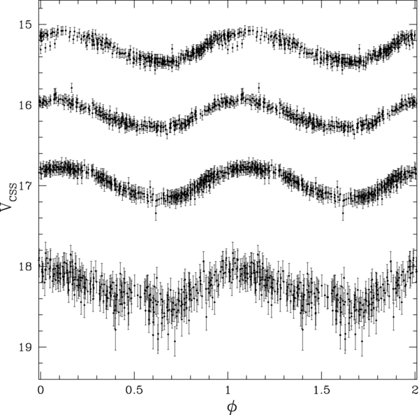
Figure 23. Light curves of RRc's with varying brightness.
Download figure:
Standard image High-resolution imageFollowing our previous analysis, we determine the distances to each of the RRc's, assuming the same absolute magnitudes for RRc's as RRab's, and using the calibration between absolute magnitude and metallicity from Catelan & Cortés (2008). As RRc light curves are nearly sinusoidal, we have not corrected the average magnitudes from the fits to static values as is necessary for the asymmetric light curve shapes of RRab's. However, a slight correction may also be necessary for RRc's (Bono et al. 1995). In Figure 24, we plot the distances to the ∼5500 RRc's detected in this analysis. The presence of RR Lyrae associated with the Sagittarius tidal stream produces a strong feature in the region 140° < R.A. < 230° at distances beyond 30 kpc, as with the RRab's in Drake et al. (2013a, 2013b).

Figure 24. Distribution of heliocentric distances for RRc's from CSDR1. The dashed lines show the location of the Sagittarius tidal stream as given by Drake et al. (2013a).
Download figure:
Standard image High-resolution imageWe found 2169 SDSS DR10 spectra matching 1136 of the RRc's in the catalog. This is a much larger fraction than RRab's with SDSS spectra (Drake et al. 2013a, 2013b), as RRc's have greater overlap with the colors of blue HB (BHB) stars. It is the BHB stars that were the targets of the SDSS SEGUE-1 and SEGUE-2 projects (Yanny et al. 2009) where they were used to determine distances based on single epochs of SDSS photometry. However, since RRc's have colors and spectra very similar to BHB's, their presence within SDSS BHB catalogs limits the overall accuracy of distances based on BHB candidates (e.g., Ruhland et al. 2011). Clean separation of BHB's and RRc's requires an assessment of variability via multiple epochs of photometry or spectra.
To compare the distances and velocities of the RRc's with the RRab's from Drake et al. (2013a, 2013b), we selected the stars with dh > 30 kpc that lie within ∼15° of the plane of the Sagittarius tidal stream as defined by Majewski et al. (2003). We found 177 RRc spectra from 146 RRc's meeting these criteria. As RRc's have much shorter periods and smaller pulsational velocities than RRab's (Liu 1991; Fernley & Barnes 1997; Jeffery et al. 2007) and the SDSS composite spectra are observed over a period of hours (Drake et al. 2013a), the radial velocities are smeared out over a range of pulsation phases. To account for this smearing, we artificially increase the measured uncertainties by 15 km s−1 since we assume that pulsation amplitudes are ∼30 km s−1.
In Figure 25, we plot the RRc Galactocentric radial velocities along with those of RRab's from Drake et al. (2013a). The new data provide additional evidence for a halo structure with a velocity component within the range 110° < R.A. < 160° as noted by Drake et al. (2013a, 2013b). This feature is not explained by the Law & Majewski (2010) model of the Sagittarius tidal stream. This was recently confirmed by Belokurov et al. (2014) based on SDSS spectra of M giants. The exact origin of this feature remains uncertain. However, it may be associated with the distant Gemini tidal stream noted by Drake et al. (2013b). Nevertheless, since the RRc's with SDSS spectra are half the distance of the most distant sources in the Gemini tidal stream, this suggests that this halo structure is dispersed over a large range of distances.

Figure 25. Distribution of Galactocentric velocities for 146 RRc's and 130 RRab's within 15° of the plane of the Sagittarius stream at distances dh > 30 kpc. The red dots are velocities of Drake et al. (2013a) RRab's, while the blue circles are RRc velocities. The small dots show the locations of simulated sources within the Sagittarius tidal stream based on the Law & Majewski (2010) model. The dashed line presents the approximate location of a velocity feature within the data first noticed by Drake et al. (2013a, 2013b) and recently confirmed by Belokurov et al. (2014) using SDSS spectra of M giants.
Download figure:
Standard image High-resolution image6.4.2. RRab's
In Drake et al. (2013a, 2013b), we discovered ∼15, 000 RRab's in CSS data. In this analysis, we examined sources with a new JWS variability threshold, as well as objects that were outside the 0.34–1.5 day period range. Based on our detection efficiency simulations, we were ∼70% complete for sources brighter than V = 17 in our original analysis. In Drake et al. (2013b), 2000 more RRab's were given and ∼2400 are from this work. Combining the total number of RRab's, we therefore expect to be 90% complete for sources with V < 17. However, we expect the completeness to be much lower for RRc's because of their generally lower variability amplitudes. In Figure 26, we present the light curves of three newly discovered RRab's.

Figure 26. Examples of light curves for three newly discovered RRab's.
Download figure:
Standard image High-resolution image6.4.3. Anomalous Cepheids or Long-Period RRab Stars
During our analysis of RR Lyrae, we discovered many long-period sources with unexpectedly high amplitudes. These objects have light curves that resemble RRab's with much shorter periods or fundamental-mode classical Cepheids. However, classical Cepheids are due to a young population and are thus limited to the Galactic plane. In Figure 27, we plot the period-amplitude distribution of the RRc's and RRab's (including those from Drake et al. 2013a, 2013b). We see that the RRab's are highly concentrated to periods <0.8 days.

Figure 27. Period–amplitude diagram for RR Lyrae. The RRab's are given by red dots and the RRc's are given by blue crosses. The dashed line shows the division used to select high-amplitude, long-period sources.
Download figure:
Standard image High-resolution imageWe selected RR Lyrae with amplitudes A > 4.3–4.3 × PF, for periods PF > 0.6 days. Based on our examination, we found some sources in this region were caused by a period alias of short-period RRab's. However, many of the light curves are sampled well enough that they are clearly not aliases of either shorter or longer period variables.
We found high-amplitude sources with periods ranging from 0.77 days to 2.4 days. Their light curves appear too similar to be due to separate types of variables. Only a slight evolution in morphology was seen with increasing period. This suggests that these sources are part of a single population.
Among the periodic variables in this group, a number were already known. Some of these sources had previously been alternately classified as Cepheids and RR Lyrae by different groups of authors. Matching these objects with SDSS, we found that the objects had the same colors as RRab's. Given the Galactic latitude limits of CSS data (|b| > 10°), the sources are unlikely to be classical Cepheids and the light curve morphology is distinctly different from that of type II Cepheids. The light curves of the objects also resemble ACEPs, which have heretofore mainly been classified in dwarf spheroidal galaxies (Coppola et al. 2013). ACEPs have periods matching those of these objects.
In Figure 28, we plot the light curves of eight ACEP variable stars. After inspection, we find 61 new variables that fall into this class. Most of the objects are brighter than V = 16 and they are distributed at Galactic latitudes ranging from 14° to 70°, with average 43°.

Figure 28. Examples of anomalous Cepheid light curves. In the top panel we plot four objects with periods 0.77–1.1 days and in the lower panel we plot sources with periods from 1.5 to 2.1 days.
Download figure:
Standard image High-resolution imageIn Figure 29, we plot the distribution of periods and Galactic latitudes of the ACEP candidates along with that of 500 classical Cepheids from the Fernie et al. (1995) catalog.14 These sources clearly have different periods and spatial distributions than classical Cepheids. Since we found no clear association between the objects and globular clusters or other sources with known distances, the absolute magnitudes of these sources remain uncertain.

Figure 29. Distribution of Cepheids. In the left panel, we plot the period distribution for the Anomalous Cepheid candidates (dashed blue line) and known classical Cepheids (solid red line). In the right panel we plot the Galactic latitude (l) distribution for the Anomalous Cepheid candidates (dashed blue line) and known classical Cepheids (solid red line).
Download figure:
Standard image High-resolution imageACEPs have been found at periods below 0.8 days in Carina (DallÓra et al. 2003; Vivas & Mateo 2013). Such stars could well be mistaken for RR Lyrae in our analysis since the distances to the sources are unknown. However, ACEPs are much rarer than RR Lyrae so we do not expect they are present in very large numbers.
6.4.4. RRd's and Blazkho RR Lyrae
RR Lyrae are known to evolve across the HB between the red and blue ends. As they do so, they cross the instability strip, becoming fundamental-mode pulsators (RRab's) on the red side and first-overtone pulsators (RRc's) on the blue side. This evolution is expected to take millions of years (e.g., Bono et al. 1997). However, apart from fundamental and first-overtone pulsators, RR Lyrae are also well known to exhibit multi-modal variations. Type d RR Lyrae (RRd's) oscillate in both the fundamental and first-overtone modes simultaneously. These two modes exhibit a period ratio of ∼0.74 between the two components (see Catelan 2009 for a review). The light curves of RRd's resemble poorly phased periodic variables. In contrast to RRd's, Blazkho RR Lyrae exhibit a modulation in amplitude and phase. Nevertheless, on long timescales, this also makes them appear like variables with poorly determined periods.
In Figure 30, we present the period–color distribution of all RR Lyrae discovered in CSS data. The RRd's have dominant single periods and colors similar to RRc's, while the Blazkhos have periods and colors similar to RRab's. Because of the possible confusion of RRd's and Blazkhos with RR Lyrae having poorly determined periods, it is likely that some of the RRd and Blazkho candidates presented here are misclassified.

Figure 30. Period–color distribution of RR Lyraes. Here we present the periods and colors for RRc's (blue crosses), RRd's (magenta triangles), RRab's (red dots), and Blazkho (black squares) RR Lyrae.
Download figure:
Standard image High-resolution imageIn addition to these sources we found six examples of RR Lyrae where the mode of pulsation appeared to change on a timescale of months. In Figure 31, we plot an example of an RR Lyrae that underwent a sudden change in amplitude and shape, from what appears in double-mode and first-overtone pulsators to that seen in fundamental-mode pulsators. The observed change in the dominant pulsation period between these two modes is only ∼21 s.

Figure 31. Light curve of a mode-changing RR Lyrae, CSSJ172304.0+290810. In the left panel, we present the light curve with the times when the system was observed in separate modes given in red and blue, respectively. In the right panel, we plot the phased light curves for the two separate pulsation modes based on the times given in the left panel.
Download figure:
Standard image High-resolution imageAdditional RR Lyrae exhibiting such changes include V442 Her (Schmidt & Lee 2000), V15 in NGC 6121 (Clementini et al. 1994), and V18 in M5 (Jurcsik et al. 2011). In the case of V18, the source was not covered continuously during the variation, so the timescale of the change is poorly determined. Both V442 Her and V18 have much shorter periods than CSSJ172304.0+290810 (0.48 days and 0.44 days, respectively). These values are consistent with RRd stars, whereas the period of CSSJ172304.0+290810 is most consistent with an RRab.
Clementini et al. (2004) also note that V21 in M68 changed from a double-mode RR Lyrae to a fundamental-mode system and then subsequently became a double-mode object again. They also note three additional RRd's in M3 (M3-V166, M3-V200, and M3-V251) that switched their dominant pulsation modes within a year. With a period of 0.59 days, CSSJ172304.0+290810 is at the limit of periods observed in double-mode RR Lyrae (Clementini et al. 2004).
Period change rates of 0.1–0.2 d Myr−1 have been observed for RR Lyrae (Le Borgne 2007). Such rates are an order of magnitude higher than predicted by stellar evolution models (e.g., Catelan 2009 and references therein). However, these have been found to be highly variable between RR Lyrae, even within individual globular clusters (Kunder et al. 2011). As noted by Kunder et al. (2011), rapid changes have been attributed to mixing events (Sweigart & Renzini 1979), magnetohydrodynamic events (Stothers 1980), and convection (Stothers 2010).
The abrupt period change for CSSJ172304.0+290810 appears to have occurred within a 120 day window, suggesting a rate of change of at least 2 days Myr−1. This is consistent with some more extreme period changes observed by Kunder et al. (2011) and Figuera Jaimes et al. (2013).
6.5. δ Scutis
δ Scuti variables can exhibit brightness variations from 0.003 to 0.9 mag in V and have periods of a few hours. High-amplitude delta Scutis (HADS, AL Velorum stars) have amplitudes greater than 0.1 mag (Alcock et al. 2000c), while low-amplitude delta Scutis (LADS) have smaller amplitudes. In Figure 32, we plot four examples of the HADS discovered. In our analysis, we are mainly sensitive to variations >0.1 mag and periods of hours where a single pulsation mode dominates, so it is likely that we did not detect all the δ Scutis within CSDR1 data. Metal-poor δ Scutis, called SX Phoenicis stars (SX Phe), are found within the halo and in globular clusters and naturally have halo velocities and metallicities.

Figure 32. Examples of high amplitude δ Scuti star light curves.
Download figure:
Standard image High-resolution imageδ Scutis often exhibit multi-periodic behavior. Most δ-Scuti variables are main-sequence stars with blue colors similar to those of RR Lyrae. This can lead to confusion for color-selected variables with insufficient sampling to determine their periods (Sesar et al. 2010). In this work, the presence of hundreds of observations and the short period (30 minutes) between sets of four observations strongly limits the misidentification of short period sources as longer period ones. For example, HADS are likely to exhibit significant variation over the span of four observations, while RRc's (which have periods of many hours), are not. The clear separatation between δ Scutis and RRc periods is shown by Palaversa et al. (2013).
Further evidence against significant δ Scuti-RRc confusion in our data comes from Figure 13. Here we again note that objects classified as RRc's have low surface gravities and low metallicities. The velocities shown in Figure SDSSvel also show that the RRc's form a halo population. Thus, the velocities, metallicities, and surface gravities rule out the presence of a significant fraction of δ Scutis (within the area covered by SDSS). On the other hand, SX Phe stars have halo population properties like RR Lyrae. Yet, as with δ Scutis, they are fainter, have higher surface gravities, and much shorter periods than the RR Lyrae (Cohen & Sarajedini 2012).
6.6. Type II Cepheids
Type II Cepheids are metal-poor Cepheids that are found in galaxy halos. These stars can be distinguished from classical Cepheids by their amplitudes, light curves, spectral characteristics, and radial velocity curves. They are fainter than classical Cepheids and are divided into three sub-classes that separated by increasing period and luminosity as defined by Wallerstein (2002).
These sub-classes are BL Herculis variables (BL Her), with periods between 1 and 5 days, W Virginis variables (W Vir) with periods of 5–20 days, and RV Tauri variables (RV Tau) with periods greater than 20 days. As with classical Cepheids, these variables can be useful for measuring distances since they obey a period–luminosity relationship (e.g., McNamara 1995; Pritzl et al. 2003; Soszynski et al. 2008).
6.6.1. BL Her
BL Her-type Cepheids usually show a bump on the descending side of their light curves at short periods. This bump is seen on the ascending side at longer periods (Soszynski et al. 2008). BL Her's have spectral types similar to RR Lyrae, but are slightly brighter. In Figure 33, we plot the light curves of a few of the BL Her-type Cepheids.

Figure 33. Examples of BL Her type variable light curves. In the top panel objects have periods from 0.89 to 1.04 days and in the lower panel 1.14 to 2.25 days.
Download figure:
Standard image High-resolution image6.6.2. W Vir and RV Tau Cepheids
W Virginis is the prototype for the population II Cepheids and has a period of 17 days. Stars in the W Vir sub-type have periods longer than 5 days and do not exhibit the bumps of BL Her stars. In contrast, RV Tau stars exhibit a secondary dip with distinctive alternating deep and shallow minima and periods longer than 20 days (Wallerstein 2002). In Figure 34, we plot examples of W Vir and RV Tau light curves within CSDR1 data.

Figure 34. Examples of W Vir and RV Tau type Cepheid light curves. Top panel: W Vir type Cepheids with periods from 6.4 to 13.9 days, Bottom panel: RV Tau-type Cepheids with periods from 22.3 to 56.9 days.
Download figure:
Standard image High-resolution image6.7. Rotational Variables
RS Canum Venaticorum variables (RS CVn's) consist of spotted stars with periods from <1 day for main-sequence stars, to hundreds of days for giants (Drake 2006). The groups of spots on these systems can give rise to periodic variations of ∼0.2 mag. However, the numbers, sizes, and locations of spots can change over time. The chromospheric activity in these stars is signaled by the presence of emission cores in the Ca ii H and K resonance lines (Fekel et al. 1986). Balmer, X-ray, and ultraviolet (UV) emission are also associated with their active chromospheres and transition regions (Engvold et al. 1988, Rodriguez-Gil et al. 2011). Most of the RS CVn's discovered in this analysis have periods longer than one day and moderately red colors consistent with the expected F- or G-type stars. In Figure 35, we present the light curves of four star rotational variable candidates.

Figure 35. Examples of rotational variable light curves.
Download figure:
Standard image High-resolution image6.8. Long-period Variables
LPVs are cool pulsating giant stars with periods ranging from a few to 1000 days. In Figure 36, we plot examples of LPV light curves. The amplitude of variation changes slightly between cycles, so the scatter in the phased light curve is greater than the actual photometric uncertainty. However, the brightest LPVs are saturated in Catalina data.

Figure 36. Examples of long period variable light curves. The brightest object among these saturates near maximum light.
Download figure:
Standard image High-resolution imageIn Figure 8 (panel 2), we noted evidence for a spatial structure distribution of LPVs in the range 135° < α < 250° from δ ∼ 30° to δ − 20°. This feature mirrors the structure observed in RRab's due to the tidal stream of the Sagittarius dwarf (Drake et al. 2013a). As this structure was originally discovered by Majewski et al. (2003) based on M giants, it is of no surprise that it is seen among red giant variables.
To demonstrate the relationship between the variables and the Sagittarius stream, we separated the LPVs by average magnitude. The brightest LPVs are foreground disk stars that are seen concentrated at low Galactic latitude, while the faintest LPVs we detected come from nearby galaxies such as M31. By selecting sources with  , we find many halo LPVs. However, LPVs have a very broad range of absolute magnitude and follow multiple families of period-luminosity relations (e.g., Fraser et al. 2005).
In Figure 37, we plot the distribution of LPVs compared to the Sagittarius stream model of Law & Majewski (2010). For the halo LPV sample, we find a significant number coinciding with the Sgr stream in the region 180° < R.A. < 245°, −20° < decl. < 15°. Approximately 50 of the 80 LPVs in the range 14.9 < V < 15.9 are found in this region. An additional eight LPVs are found in the region 50° < R.A. < 80°, −10° < decl. < 30° which also overlaps with the Sgr stream.

Figure 37. Distribution of LPVs compared to the Law & Majewski (2010) model of the Sagittarius stream. The large blue dots show LPVs with 14.9 < V < 15.9 and the green boxes show the locations of all other LPVs. The dashed line shows the plane of the Sgr stream system defined by Majewski et al. (2003). The red points show the locations of simulated Sgr stream sources from Law & Majewski (2010).
Download figure:
Standard image High-resolution imageTo further test the association of LPVs with the Sagittarius stream we selected LPVs within 15° of the plane of the Sagittarius stream system defined by Majewski et al. (2003). In Figure 38, we plot the locations of these objects.

Figure 38. Spatial distribution of LPVs within 15° of the plane of the Sagittarius tidal stream region. In the bottom panel we plot the average magnitudes for LPVs. In the top panel we plot distances assuming the LPVs have MV = −3. The dashed lines show the location of the Sagittarius streams as given by Drake et al. (2013a).
Download figure:
Standard image High-resolution imageUnder the assumption that LPVs have representative luminosities of around MV = −3 (Smak 1966) in CSDR1 data, we find good agreement with the results based on RRab's and RRc's. However, LPVs are known to occupy six separate period–luminosity sequences (Fraser et al. 2005) and perhaps more (Mosser et al. 2013). As many of the LPV sequences overlap in period range, to derive more accurate absolute magnitudes, hence distances, one must first determine the sequence of the variable. A combination of light curve morphology and multi-wavelength observations may enable this determination. Nevertheless, the figure does show that there is a strong trend in the average brightness of LPVs, which is consistent with membership of the Sagittarius tidal stream.
6.9. Miscellaneous Variable Sources
More than 99% of the periodic variables inspected clearly fall into to the types described above. However, some of the periodic variables are difficult to classify. In Figure 39, we plot the light curves of six periodic variables with uncertain classifications. The top two light curves in the left panel are indicative of objects that exhibit zigzag shapes yet vary from one object to the next. The lower two light curves in this panel exhibit smoother curves that may be indicative of overcontact systems sharing a common envelope. The light curves in the right panel of Figure 39 exhibit some of the features of contact binaries presenting the O'Connell effect. However, the shapes of these "Hump" variables are much more erratic. This may be due to the presence of gas streams or hot spots on their surfaces, such as noted by Wilsey & Beaky (2009). In total there are 68 objects in this group of which 25 are placed in the Hump group.

Figure 39. Light curves of unclassified periodic variables. The objects in the left panel have periods of 0.19 days (red), 0.25 days (blue), and 0.28 days (green). The objects in the right panel have periods of 0.42 days (red), 0.45 days (blue), and 0.80 days (green).
Download figure:
Standard image High-resolution imageDuring inspection of the periodic candidates in this work, we discovered a number of nonperiodic sources and periodic sources where the light curve did not fit any of the existing classifications. Most of the nonperiodic variables are simply stars and QSOs exhibiting irregular variability. However, some sources exhibiting outbursts were also discovered. Among the aperiodic sources, we serendipitously detected 51 supernovae, of which 42 are new discoveries. Eighteen of these SNe occurred during the operation of CRTS (Drake et al. 2009) and other large transient surveys such as PTF (Law et al. 2009) and PanSTARRS-1 (Hodapp et al. 2004). The discovery of such a large fraction of new SNe suggests that current transient surveys miss many nearby, bright supernovae. Further details of the sources are given in the appendices.
7. COMPLETENESS, ACCURACY, AND PURITY
One possible way of measuring the utility of a periodic variable star catalog is based on its purity, accuracy, and completeness. A natural expectation is that a periodic variable catalog should consist purely of stellar sources. Additionally, the catalog sources should provide accurate periods, magnitudes, amplitudes, and classifications. One might also expect a level of completeness that is at minimum equivalent to other recent catalogs.
7.1. Purity
To determine the purity of our periodic variables, we matched our initial candidates with sources in SDSS DR10 photometry and spectroscopic catalogs (3'' radius). Among the spectroscopic matches, there were 83 different types of spectra recorded in SDSS. These types can be broadly separated into stars, galaxies, and QSOs. In Table 4, we present the number of sources with SDSS photometry and spectra data among the 112,000 pre-inspection candidates and among selected sources. This table shows that a large number of the initial periodic candidates had spectra classifying them as galaxies and QSOs. However, as expected, after the light curves were inspected, only a few were selected as periodic variables.
Table 4. SDSS Classes of Periodic Candidates
| Spectroscopic Types | I | S |
|---|---|---|
| Total | 5420 | 2299 |
| Star | 2918 | 2256 (2291a) |
| Galaxy | 1659 | 38 (3a) |
| QSO | 843 | 5 (5a) |
| Photometric Types | I | S |
| Total | 67076 | 27871 |
| Star | 58443 | 25639 |
| Galaxy | 5593 | 827 (∼10a) |
| Unknown | 3040 | 1405 |
Notes. Numbers and SDSS-DR10 object types from Catalina periodic variable candidates with SDSS photometry and spectra. Column 1: SDSS object type. Column 2: number of SDSS matches among the 112,000 inspected periodic variable candidates. Column 3: number of SDSS sources selected as periodic variables before inspection of SDSS images and spectra. aNumber based on inspection of SDSS data.
Download table as: ASCIITypeset image
We reviewed the SDSS spectra for the 38 objects marked as galaxies and five sources marked as QSOs. Twenty-eight of the spectra marked as galaxies were G and K stars that were incorrectly classified as galaxies near redshift zero. Seven of the matches were due to variables blended with neighboring faint galaxies. Only three sources were actually galaxies. These objects were removed from the catalog. All five of the objects classified as QSOs by SDSS were systems with strong emission lines. Two of the active galactic nuclei (AGNs) among these appeared to exhibit possible periodic variability, yet all were removed. The possible periodic variability of the two AGNs may be due to an unresolved variable superimposed on the galaxies.
Based on the total number of SDSS spectra, the false classification rate suggests that ∼0.3% (8/2299) of the objects in the catalog are likely to be galaxies or QSOs. Thus, from the whole catalog, one might expect ∼160 such objects. However, SDSS used color selection to choose targets for spectroscopic follow-up. Within SDSS-DR10, more than two million spectra of galaxies and QSOs have been taken, compared with only ∼270, 000 stars (see: http://www.sdss3.org/dr10/). This suggests that the spectra comprise a much more complete sample of QSOs and galaxies than stars, so the number of non-stellar sources may actually be smaller.
In contrast to the SDSS spectroscopy, photometry has been undertaken by SDSS across a large fraction of the sky irrespective of the source type. This imaging provides much greater depth and resolution than CSS data, as well as multi-band photometry. This makes it an ideal source for investigating even the faintest of the CSDR1 variables. In order to further test the purity of our sources we matched the periodic candidates with object in the SDSS-DR10 photometric catalog. Approximately 28,000 of the sources from our periodic variable catalog have SDSS photometry. Additionally, every object in SDSS is classified as either a star, a galaxy, or an object of unknown type. As with the SDSS spectra, there were many sources marked as galaxies among our initial candidates. However, a moderate number (∼3%) of the objects that we classified as periodic variables were classified by SDSS as galaxies.
Upon inspection of the SDSS images, we found that the automated SDSS classifications were generally incorrect. For example, 77% of the catalog sources marked as galaxies had VCSS < 15. These objects were found to be stars that were saturated in SDSS photometry rather than actual galaxies. It seems likely that the saturation causes the sources to appear extended and thus to be wrongly classified as galaxies. Nevertheless, in order to account for differences in the saturation limit within the five SDSS photometry bands, and for variation in star color, we examined the SDSS images of all 386 objects marked as galaxies with VCSS > 14. Only 10 of these sources were found to be galaxies. These objects were removed from the catalog.
We also reviewed the SDSS images for some faint variables that were marked as galaxies by SDSS. In contrast to the saturated sources, almost all of the sources fainter than VCSS = 15 were found to be blends between close pairs or groups of stars, although there were also a few cases where a periodic variable was blended with a galaxy. More than a dozen of the faint sources classified as galaxies based on SDSS photometry had stellar SDSS spectra. We found that in many cases the objects marked as galaxies had multiple epochs of SDSS photometry where sources were alternatively marked as stars or galaxies depending on seeing. Based on an inspection of SDSS images and the photometric color information, we find ≪0.1% of the periodic catalog sources are in fact galaxies. However, since QSOs are marked as stars in SDSS photometry, it is likely that there is some contamination due to QSOs (as suggested by the SDSS spectra above). We have removed all the definitive galaxies and QSOs from the catalog.
7.2. Completeness and Accuracy
7.2.1. Known Variables from VSX
The International Variable Star Index (VSX; Watson et al. 2006) provides what is very likely the most complete catalog of known variable stars. We matched the original 154, 000 CSDR1 periodic variable candidates with sources in the VSX data set and found 6459 matches. These objects come from 176 different classes of variable stars. This very large number of classes is due to subclasses of variables as well as sources having either multiple or uncertain classifications (e.g., class EB-EW, signifies membership of either β Lyrae or W UMa types). However, many of the variable stars within the VSX catalog are not specifically periodic or they have nonperiodic outbursts (e.g., T Tauri stars, YSOs, CVs, AM CVn's). Therefore, we do not expect to recover all of the VSX variables.
The VSX variable classes having more than 100 matching variables of one type include: eclipsing binaries (3201), RR Lyrae (1006), δ Scutis (240), U Geminorum-type variables (214), Mira (206), and miscellaneous variables with unknown variable types (382). Of the original periodic candidates, 6030 were among the 112, 000 periodic variable candidates that were inspected. Of these, 4861 made it into the final catalog. In Table 5, we present the number of known variables of each main type passing our initial and final selections.
Table 5. Matches with VSX Sources
| Var Type | O | I | S |
|---|---|---|---|
| All | 6454 | 6030 | 4861 |
| EB | 3201 | 3070 | 2834 |
| RR Lyrae | 1006 | 958 | 925 |
| δ Scuti | 240 | 234 | 210 |
| U Gem | 214 | 119 | 6 |
| Mira | 206 | 187 | 162 |
| Misc | 382 | 328 | 217 |
Notes. Column 1: main types of variables with VSX matches. Column 2: number of VSX variables of each type among the original 154,000 periodic candidates. Column 3: number of VSX variables in the inspected set of 112 thousand candidates. Column 4: number of VSX variables selected for final periodic variable catalog. We include both MISC and VAR VSX classes in our Misc category.
Download table as: ASCIITypeset image
Unsurprisingly, many of the stars missing from the catalog are dwarf novae (U Gem type). These are not in our catalog since their light curves are dominated by large outbursts that occur at times that are quasi-periodic at best. The light curves of these known CVs are available through the Catalina Web site.
Approximately 89% of the strictly periodic variables (eclipsing binaries, RR Lyrae, and δ Scutis) with VSX matches among our original candidates were recovered, and 93% of the periodic candidates passing our periodic candidate selection are within our final catalog. As a comparison, we found only 1144 matches to the much smaller GCVS variable star catalog (Samus et al. 2002–2013; 2013 June edition). Since the GCVS variable catalog is included within the VSX set, we do not consider it further.
7.2.2. Comparison with LINEAR
While the VSX catalog provides a very complete set of known variables stars, it is inherently heterogeneous (being derived from hundreds of authors using hundreds of different instruments). Therefore, to test the accuracy of our catalog, we instead decided to compare our results with large sets of variable stars found using a single instrument.
Palaversa et al. (2013), undertook the analysis of 200,000 variable star candidates selected from the 25 million objects observed by the LINEAR experiment. They detected 7196 periodic variables in the range 14.5 < mlinear < 17 from a ∼10, 000 deg2 region of the sky overlapping SDSS. In contrast to this work, where all 112, 000 candidates were inspected by a single person (A.J.D.), the LINEAR analysis consisted of combining the results from eight people who each inspected ∼25, 000 different light curves. In order to mitigate the biases of combining the separate classifications, Palaversa et al. (2013) reviewed all of the final candidates.
The LINEAR classification scheme consists of 11 types. Among these classes, the three least populated have a combined total of only 12 variables. In comparison with this work, the LINEAR classification scheme does not include any ellipsoidal or rotational variables (e.g., spotted stars such as RS CVn's) which account for >3% (>1500 objects) of our periodic variables. It also does not include Blazkho's, RRd's, or PCEBs (WD and SD binaries). Such systems are also not included within their "Other" class.
In order to first determine the completeness of our survey compared to Palaversa et al. (2013), we matched the coordinates of our candidate periodic variables with LINEAR variables within 3''. Due to differences in the sky coverage of the two surveys, 6750 of the LINEAR variable stars with periods were covered by CSDR1. We found that only 645 (9.6%) of the LINEAR objects were not in our initial selection. Of the missing LINEAR variable stars, 60 were found to have an amplitude <0.1 mag in CSDR1. Most of the other missing sources were in areas having few observations in the CSDR1 data.
In our final periodic variable catalog, we found that 6016 of the 6750 (89%) LINEAR periodic variables were included. This result is in good agreement with the completeness based on the VSX catalog above. However, since VSX and LINEAR data is magnitude-limited, we expect that our completeness is much lower below VCSS = 17.
In order to compare the classifications given by LINEAR, we matched each type of variable given by Palaversa et al. (2013) with those from our catalog (including Type ab and Blazkho RR Lyrae from Drake et al. 2013a, 2013b). In Table 6, we present a so-called confusion matrix for the 6016 objects in common. The agreement between the two classifications is very good, with 94% of the objects having the same classification. The sources with different classifications include a number of β Lyrae, RRd's, and Blazkho RR Lyrae for which the Palaversa et al. (2013) catalog has no classification. Ignoring the 171 objects in the missing classes, the agreement is excellent, at ∼97%.
Table 6. Catalina Variables with LINEAR Matches
| Type | BLHer | ACEP | δ-Scuti | EA | EB/EW | LPV | Misc | RRab | RRc |
|---|---|---|---|---|---|---|---|---|---|
| Cep-II | ... | ... | ... | ... | 2 | 1 | 1 | 1 | ... |
| ACEP | 4 | ... | ... | ... | ... | ... | ... | 2 | ... |
| HADS | ... | ... | 14 | ... | ... | ... | ... | ... | ... |
| LADS | ... | ... | ... | ... | ... | ... | ... | ... | ... |
| EA | ... | ... | ... | 226 | 86 | ... | ... | ... | ... |
| EW | ... | ... | ... | 18 | 1943 | ... | 2 | ... | 14 |
| β Lyrae | ... | ... | ... | 1 | 27 | ... | ... | ... | ... |
| ELL | ... | ... | ... | ... | 3 | ... | ... | ... | ... |
| LPV | ... | ... | ... | ... | ... | 48 | ... | ... | ... |
| RRab | ... | 2 | ... | ... | 2 | ... | 6 | 2640 | 18 |
| RRc | ... | ... | ... | ... | 9 | ... | 2 | 5 | 773 |
| Blazkho | 1 | ... | ... | ... | ... | ... | 1 | 38 | 3 |
| RRd | ... | ... | ... | ... | 1 | ... | 5 | 6 | 96 |
| RS CVn | ... | 1 | ... | ... | ... | 2 | 1 | 1 | ... |
| PCEB | ... | ... | ... | 2 | ... | ... | ... | ... | ... |
| Hump | ... | ... | ... | ... | 1 | ... | ... | ... | 1 |
| EAUP | ... | ... | ... | 4 | ... | ... | ... | ... | ... |
| PU | ... | ... | ... | 1 | 1 | ... | ... | ... | ... |
Notes. The first row gives the types of periodic variable from Palaversa et al. (2013) based on LINEAR data, and the first column gives the classes based on the current analysis.
Download table as: ASCIITypeset image
Aside from the results above, we note that the LINEAR catalog classifies 20 objects as EAs with single eclipses. Only five of these objects match sources in our catalog. Four of the systems were found to have two eclipses with a significant difference in eclipse depth. The remaining EA appears to have two eclipses of similar depth. Three of the EAs were found to have been phased at half their true periods, thus explaining the single eclipses. All of the eclipsing binaries in our catalog are given at periods that provide two eclipses since it is very common for single eclipses to appear when light curves are phased to half their true periods.
As the classes of variables are in excellent agreement, we can also compare the periods, amplitudes, and magnitudes of the matching objects. Both LINEAR and CSS observations are taken unfiltered. In Figure 40 we compare the median LINEAR magnitudes with the average Fourier fit magnitudes from CSDR1. Once again, we find excellent agreement between the two systems over the magnitude range of the LINEAR variables. In Figure 41, we compare the variation amplitudes measured by LINEAR with those from our Fourier fits. Palaversa et al. (2013) determined the amplitude as the range of points between 5% and 95% in the magnitude distribution. In detached binaries systems, eclipses can last <10% of the orbital period, so we expect that the Palaversa et al. (2013) scheme will often underestimate the actual amplitude for such objects. However, as these are only 4% of the matching variables, the LINEAR and CSS amplitudes are in good agreement. For variables with small amplitudes, the LINEAR values are generally slightly larger. This is likely to be due to cases where the uncertainty in the measurements is comparable with the amplitude of variability. At the low-amplitude limit, the distribution of photometric measurements between 5% and 95% represents the photometric scatter rather than the amplitude of variability.

Figure 40. Comparison of median magnitudes for variables found in LINEAR data with CSS magnitudes.
Download figure:
Standard image High-resolution image
Figure 41. Amplitudes of variables discovered in LINEAR compared to the values from Fourier fits to CSS data.
Download figure:
Standard image High-resolution imageIn Figure 42, we compare the periods determined by Palaversa et al. (2013) with this work over the range where >90% of the variables reside. The apparent features present below 0.4 days are merely due to the periods being rounded to the sixth decimal place. Overall, the differences in the periods are generally <0.002%. Once again, this suggests excellent agreement and independent confirmation of the variables. Combining the VSX and LINEAR catalogs, we find that, overall, 7856 objects were previously known periodic variables. The remaining ∼39, 000 are new discoveries.

Figure 42. Period comparison. The percentage difference in period for sources present in both the LINEAR catalog (Palaversa et al. 2013) and this work, as function of the periods derived in this work. The features below 0.4 days are artifacts due to rounding.
Download figure:
Standard image High-resolution image7.3. Comparisons with Other Variability Surveys
The largest existing sources of variable stars are microlensing surveys. Together, the four OGLE microlensing surveys (I–IV; Udalski et al. 1994) have run for more than 20 years in search of microlensing events toward the Bulge and the Magellanic Clouds. As a by-product, the OGLE I-III surveys have detected more than 200,000 periodic variables (e.g., Soszynski et al. 2009a, 2009b, 2010a, 2010b, 2011a, 2011b; Graczyk et al. 2011; Pawlak et al. 2013). Most of the variable stars have been found within the Magellanic Clouds. Similarly, over a hundred thousand periodic variables have been discovered in data from the Macho microlensing project that was also taken toward the LMC and Bulge fields (e.g., Alcock et al. 1996, 1997, 1998, 1999, 2000b, 2001, 2002; Faccoli et al. 2007; Fraser et al. 2008). Many of the variables detected by these surveys are common due to this overlap. Combined, these surveys cover <1000 deg2 on the sky.
Coverage of the Galactic Bulge is now being expanded into the high extinction regions by the VVV survey which also monitors the inner Galactic Disk for variability in the near-IR (Minniti et al. 2010; Catelan et al. 2011). This will ultimately cover 562 deg2 in Z, Y, J, H, and Ks (Saito et al. 2012). Discoveries already include RR Lyrae, Cepheids, eclipsing binaries, LPVs, and rotational binaries (Catelan et al. 2013).
Over larger and less crowded regions of the sky, the very wide-field cameras of the ASAS survey (Pojmanski 1997) have discovered tens of thousands of variable stars down to V ∼ 14 (e.g., Pojmanski 2000, 2002, 2003; Pojmanski & Maciejewski 2004a, 2004b; Pojmanski et al. 2005; Richards et al. 2012). The NSVS survey has also covered a large fraction of the sky to a similar depth (8 < V < 15.5; Wozniak et al. 2004) using the Robotic Optical Transient Search Experiment (ROTSE-I; Akerlof et al. 2000). Searches of the ROTSE data by Kinemuchi et al. (2006) and Hoffman et al. (2008, 2009) have revealed many thousands of periodic variables.
Deeper searches for variability, in much smaller fields, have been carried out by QUEST (Vivas et al. 2004), LONEOS (Miceli et al. 2008), MOTESS-GNAT-1 (MG1; Krauss et al. 2007), Kepler (Matijevic et al. 2012), and SDSS Stripe-82 (Sesar et al. 2007; Bhatti et al. 2010, Becker et al. 2011).
In Table 7, we compare the search parameters for surveys that have discovered large numbers of periodic variables stars. While this table is not exhaustive, it does show that the CSDR1 is currently unequaled in its combination of sky area and depth. However, as microlensing surveys cover a similar number of stars within much smaller areas and are observed at much higher cadence, it is not surprising that they continue to dominate the discovery statistics.
Table 7. Periodic Variables from Large Surveys
| Survey | Sources |  |
Area | Range | Span | Epochs | Filters |
|---|---|---|---|---|---|---|---|
| (106) | (deg2) | (mag) | (yr) | ||||
| OGLE I-III | 20–200 | >200,000 | 100–630 | 12–21 | 21 | 200–5000 | V, I |
| MACHO | 60 | ∼120,000 | 100 | 13–19.5 | 8 | 150–2000 | V, R |
| CSDR1 | 200 | 61,000a | 20,000 | 12.5–19.5 | 7 | 70–350 | C |
| ASAS | 15 | 12,000 | 30,000 | 8–14 | 9 | 540 | V, I |
| LINEAR | 25 | 7000 | 10,000 | 14–17 | 9 | 250 | C |
| NSVS | 14 | 5600 | 30,000 | 8–15.5 | 1 | 100–500 | C |
| MG-1 | 2.1 | 5200 | 300 | 13–19 | 2 | 200 | R |
| Kepler | 0.13 | 2600 | 116 | 9–16 | 3.5 | >50,000 | C |
| LONEOS | 1 | 840 | 1430 | 13–18.5 | 2 | 28–50 | C |
| Quest | 1.2 | 500 | 380 | 13.5–19.7 | 2.3 | 15–40 | U, B, V, R, I |
| SDSS Stripe-82 | 1 | 500 | 290 | 15–21 | 3 | 70 | u, g, r, i, z |
Notes. The number of periodic variables discovered by major projects based on references given within the text. Column 1: names of survey where the data was taken. Column 2: number of sources covered by survey. Column 3: number of known periodic variables. Column 4: total sky coverage. Column 5: range of survey photometry magnitudes. Column 6: total time span of the survey observations. Column 7: number of image epochs taken per band. Column 8: observation bands (C = clear/no filter). Note: the data searched within the NSVS and LONEOS data is a small fraction of the total data taken by these surveys. aIncluding RRab's from Drake et al. (2013a, 2013b).
Download table as: ASCIITypeset image
8. DISCUSSION AND CONCLUSIONS
In this paper, we have presented an extensive search for periodic variable sources among 5.4 million candidate variables selected from the CSDR1 data set. When combined with variables from our prior analysis (Drake et al. 2013a, 2013b), the resulting catalog includes more Galactic eclipsing binaries and RR Lyrae than any existing survey. Comparison between catalog sources and previously known periodic sources leads to the recovery of ∼90% of known periodic objects in the observed fields. Of the 46,668 periodic variables detected, 38,812 (82%) are new discoveries. Additionally, 396 of these variables are detected twice due to overlap between fields. The high percentage of new discoveries is not unexpected since this analysis covers more area to a greater depth than any past search for periodic variables. Our variable star catalog does not include ∼4800 sources that were flagged as potential periodic variables during the light curve inspection process.
Among the ∼31, 000 contact and ellipsoidal binaries, we find almost 400 systems with periods below the 0.22 day cutoff. These sources will be investigated in an upcoming paper (Drake et al. 2014a). We also find many contact binaries that exhibit the O'Connell effect. The presence of stable light curves over >2000 days suggests that this effect is not due to star spots. The presence of long-timescale variations due to spots can be seen among other contact binaries, providing further evidence that the O'Connell effect is not due to star spots.
We have investigated the possibility that contact binaries may have been misidentified as RRc's within our catalog. Based on WISE and SDSS photometry as well as SDSS spectra, we find that the misidentification rate is, at most, a few percent within our catalog. This result suggests that RRc's can be used as probes of halo structure without significant contamination. Using the RRc's, we confirm the presence of the Sagittarius tidal stream structures. Additionally, we find strong evidence that a large fraction of the LPVs that we have discovered are part of the Sagittarius tidal stream.
We have found a small number of RR Lyrae that appear to undergo a rapid change in their pulsation mode. Clementini et al. (1994) called these objects switching-mode pulsators. The presence of sudden (<120 days) changes may suggest abrupt changes to the stellar interior. Analysis of CSSJ172304.0+290810 suggests that some switching-mode pulsators are not Blazkho or RRd variables. However, more detailed analysis is required to fully test these possibilities.
In this analysis, we have detected 85 PCEB candidates, of which 45 are new discoveries. Parsons et al. (2013) recently investigated PCEBs using Catalina data. They selected candidate eclipsing systems based on the light curves of 835 spectroscopically confirmed WD-dM binaries. They found 29 new eclipsing systems, bringing the total number of known systems to 49. They also found 13 noneclipsing ellipsoidal systems. Unlike the Parsons et al. (2013) analysis, our selection is not limited to sources with SDSS spectra. However, our ability to find such systems is strongly biased by the presence of modulations within the light curve. Only nine of the Parsons et al. (2013) systems are re-detected, since PCEBs without modulations, such as those discovered by Drake et al. (2010), cannot be detected. The current analysis, like that of Parsons et al. (2013), is thus biased toward the detection of PCEB systems containing a luminous secondary.
We have detected a significant population of fundamental-mode pulsators with light curves that resemble both RRab's and classical Cepheids. These sources have amplitudes that are significantly larger than RRab's at their observed periods and extend well beyond RR Lyrae (up to 2.5 days). These sources have a significantly smaller range of periods and a larger range of Galactic latitude than known classical Cepheids. They also do not exhibit the bumps seen among short-period type II Cepheids. We suggest that these objects are either ACEPs or RR Lyrae that have recently evolved off the HB.
We are currently in the process of analyzing variable sources detected in data taken by the MLS and SSS telescopes available in CSDR2. In this work, we have parameterized Catalina light curves based on statistical features such as periodicity, amplitude, variance, etc. The current catalog will provide a training set for selecting periodic variables within CSDR1 via Artificial Neural Networks, Random Forests, and Support Vector Machines following work performed to classify transient events (Mahabal et al. 2011; Djorgovski et al. 2012; Donalek et al. 2013). In addition, we will apply Self-Organizing Maps and other machine learning techniques, similar to approaches that recently have been applied to large sets of variable stars (e.g., Dubath et al. 2011; Blomme et al. 2011; Richards et al. 2012; Palaversa et al. 2013).
In this analysis, we have exclusively searched for periodic variables in the sparse stellar fields that are observed away from the Galactic Disk. Extensive variability searches have also been undertaken in the Bulge and toward the Magellanic Clouds as a by-product of microlensing surveys. However, the dense stellar fields of the Galactic Disk remain largely unprobed for periodic variable stars.
In the near future, the Gaia mission (Perryman et al. 2001) and the VVV survey (Minniti et al. 2010) will begin to harvest Galactic disk fields and are expected to find millions of periodic variables (Eyer et al. 2012; Catelan et al. 2013). Although Gaia is only expected to reach stars to the same depth and number of epochs as CSDR1, it is expected to have ultra-precise photometry. This will greatly increase the number of periodic variables discovered even within CSDR1 fields since the fraction of variables increases as a power law with increasing photometric precision (Huber et al. 2006; Howell 2008). Likewise, while the LSST survey will have similar total numbers of observations (Ivezic et al. 2008), it will reach far greater depths than any existing wide-field survey. LSST will thus find millions of faint periodic variable sources.
CRTS and CSDR1 are supported by the U.S. National Science Foundation under grant AST-1313422. The CSS survey is funded by the National Aeronautics and Space Administration under grant No. NNG05GF22G issued through the Science Mission Directorate Near-Earth Objects Observations Program. J.L.P. acknowledges support from NASA through Hubble Fellowship Grant HF-51261.01-A awarded by the STScI, which is operated by AURA, Inc. for NASA, under contract NAS 5-26555. Support for M.C. and G.T. is provided by the Ministry for the Economy, Development, and Tourism's Programa Iniciativa Científica Milenio through grant IC120009, awarded to the Millennium Institute of Astrophysics (MAS); by Proyecto Basal PFB-06/2007 and by Proyecto FONDECYT Regular #1110326 and #1141141. SDSS-III is managed by the Astrophysical Research Consortium for the Participating Institutions of the SDSS-III Collaboration. Funding for SDSS-III has been provided by the Alfred P. Sloan Foundation, the Participating Institutions, the National Science Foundation, and the U.S. Department of Energy Office of Science. The SDSS-III Web site is http://www.sdss3.org/. This research has made use of the International Variable Star Index (VSX) database, operated at AAVSO, Cambridge, MA, USA.
APPENDIX A: SUPERNOVAE
During inspection of the periodic candidates in this work, we discovered a number of nonperiodic sources and periodic sources where the light curve did not fit any of the existing classifications. Most of the nonperiodic variables are simply stars and QSOs exhibiting irregular variability. However, some sources exhibiting outbursts were also discovered.
Our review of periodic candidates led to the discovery of 51 variable sources exhibiting single, long, outbursts. Closer inspection showed that sources were supernovae associated with galaxies seen in SDSS and Catalina images. Nine of these objects were previously discovered SNe, while the rest were new discoveries. Since supernovae are clearly not periodic, their discovery among our candidates is purely serendipitous. However, this is not completely unexpected since Palaversa et al. (2013) discovered a supernova during their inspection of periodic variable candidates from LINEAR data. In Table 8, we present the parameters of the 42 newly discovered supernovae. Among all the supernovae discovered, two have SDSS spectra where some flux from the SN is seen. In one case, this led to the host galaxy being classified by SDSS as a QSO.
Table 8. Parameters of Newly Discovered Supernovae
| CRTS ID | R.A. | Decl. (J2000) | UT Date | z |
|---|---|---|---|---|
| CSS_J221632.6−020841 | 22:16:32.67 | −02:08:41.2 | 2005 Sep 24 | ... |
| CSS_J021056.9+362733 | 02:10:56.92 | +36:27:33.9 | 2005 Oct 25 | ... |
| CSS_J035255.3−112753 | 03:52:55.33 | −11:27:53.5 | 2005 Nov 2 | ... |
| CSS_J235535.6+291220 | 23:55:35.62 | +29:12:20.4 | 2005 Nov 20 | ... |
| CSS_J044104.9+093109 | 04:41:04.90 | +09:31:09.4 | 2005 Nov 25 | ... |
| CSS_J092459.1+013839 | 09:24:59.17 | +01:38:39.2 | 2005 Dec 28 | ... |
| CSS_J050141.1−015936 | 05:01:41.19 | −01:59:36.2 | 2005 Dec 31 | ... |
| CSS_J162513.0+112756 | 16:25:13.06 | +11:27:56.0 | 2006 Mar 24 | ... |
| CSS_J123716.5+264710 | 12:37:16.59 | +26:47:10.9 | 2006 Apr 26 | ... |
| CSS_J023657.0+192258 | 02:36:57.06 | +19:22:58.0 | 2006 Nov 11 | ... |
| CSS_J102255.7+163606 | 10:22:55.71 | +16:36:06.4 | 2006 Dec 14 | 0.0449 |
| CSS_J112851.2+390458 | 11:28:51.24 | +39:04:58.7 | 2007 Feb 27 | ... |
| CSS_J141731.1+431843 | 14:17:31.16 | +43:18:43.0 | 2007 Mar 11 | ... |
| CSS_J113517.2−152048 | 11:35:17.23 | −15:20:48.8 | 2007 Mar 30 | ... |
| CSS_J144959.8+084819 | 14:49:59.89 | +08:48:19.6 | 2007 Apr 11 | ... |
| CSS_J130404.0+443720 | 13:04:04.08 | +44:37:20.3 | 2007 Jun 16 | ... |
| CSS_J013303.2−082303 | 01:33:03.28 | −08:23:03.6 | 2007 Sep 6 | ... |
| CSS_J014920.9+313213 | 01:49:20.94 | +31:32:13.6 | 2007 Sep 12 | ... |
| CSS_J090316.2+373746 | 09:03:16.25 | +37:37:46.4 | 2007 Nov 20 | ... |
| CSS_J083533.4+015103 | 08:35:33.48 | +01:51:03.2 | 2007 Dec 17 | ... |
| CSS_J152459.7+045422 | 15:24:59.73 | +04:54:22.7 | 2008 Jan 9 | 0.04373 |
| CSS_J161542.7+332401 | 16:15:42.77 | +33:24:01.0 | 2008 Feb 12 | 0.02969 |
| CSS_J151555.7+165902 | 15:15:55.75 | +16:59:02.4 | 2008 Apr 15 | ... |
| CSS_J221502.0+151854 | 22:15:02.00 | +15:18:54.2 | 2008 Sep 22 | ... |
| CSS_J100004.1+060544 | 10:00:04.18 | +06:05:44.7 | 2008 Dec 6 | ... |
| CSS_J085423.4+512330 | 08:54:23.41 | +51:23:30.1 | 2009 Feb 24 | ... |
| CSS_J141043.2+115704 | 14:10:43.22 | +11:57:04.5 | 2009 Mar 18 | ... |
| CSS_J224534.9+263535 | 22:45:34.94 | +26:35:35.8 | 2009 Jul 31 | ... |
| CSS_J011524.5−100823 | 01:15:24.54 | −10:08:23.5 | 2009 Sep 16 | ... |
| CSS_J020949.5+294021 | 02:09:49.56 | +29:40:21.7 | 2009 Sep 18 | ... |
| CSS_J073643.3+473127 | 07:36:43.32 | +47:31:27.5 | 2009 Nov 14 | ... |
| CSS_J114817.6+292102 | 11:48:17.61 | +29:21:02.3 | 2009 Nov 24 | 0.0476 |
| CSS_J020439.7+130902 | 02:04:39.76 | +13:09:02.9 | 2009 Dec 7 | ... |
| CSS_J103418.6+225056 | 10:34:18.65 | +22:50:56.2 | 2009 Dec 16 | ... |
| CSS_J133147.6+072652 | 13:31:47.69 | +07:26:52.8 | 2010 Mar 15 | 0.0209 |
| CSS_J145206.1+175523 | 14:52:06.12 | +17:55:23.3 | 2010 Mar 19 | ... |
| CSS_J151658.3+052245 | 15:16:58.32 | +05:22:45.3 | 2010 May 6 | ... |
| CSS_J081617.0+014822 | 08:16:17.04 | +01:48:22.5 | 2010 Oct 19 | ... |
| CSS_J090424.8+210542 | 09:04:24.89 | +21:05:42.6 | 2010 Dec 1 | ... |
| CSS_J101727.6+155844 | 10:17:27.62 | +15:58:44.5 | 2011 Jan 13 | ... |
| CSS_J082143.2+034733 | 08:21:43.25 | +03:47:33.1 | 2011 Jan 13 | 0.02975 |
| CSS_J132915.1+154719 | 13:29:15.19 | +15:47:19.2 | 2011 Mar 5 | ... |
Notes. Column 1: Catalina ID. Columns 2 and 3: right ascension and declination. Column 4: date of maximum light. Column 5: host galaxy redshift (if known).
Download table as: ASCIITypeset image
To contrast these new detections with ongoing efforts to discover supernovae and other transients in the CSS data, we note CRTS has so far discovered >1, 000 supernovae in seven years of CSS data. The fact that half of the new supernovae occurred during the operation of CRTS, but were not detected, was found to be due to their association with luminous host galaxies. In most cases, the increase in total brightness of the galaxy plus supernovae is <1.5 mag. This is insufficient for automated detection by CRTS (Drake et al. 2009). In the near future, the CRTS-II project will undertake image subtraction to find such supernovae. Our results suggest that the current detection rate should increase significantly.
In Figure 43, we present the light curves of four of the newly discovered supernovae. We also show the apparent brightness of these events after the flux from the host galaxy has been subtracted.

Figure 43. Light curves of serendipitously discovered supernovae. Left: observed SN plus host galaxy light curve. Right: light curve of the SN after subtracting the constant host galaxy flux.
Download figure:
Standard image High-resolution imageAPPENDIX B: CATACLYSMIC VARIABLES
In addition to supernovae, we discovered 18 new dwarf nova-type CVs. The light curves of these objects exhibit repeated outbursts. In Figure 44, we plot two of the sources and in Table 9, we present the details of outbursting CVs discovered during the analysis. Drake et al. (2014b) found that almost all CVs discovered by CRTS have u − g < 0.6 and g − r < 1. Four of the eighteen new CVs covered by SDSS photometry exhibit color excess compared to Drake et al. (2014b). This suggests CV systems where the companion star dominates the observed flux.

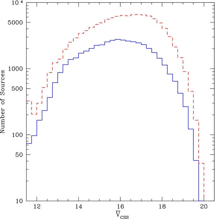
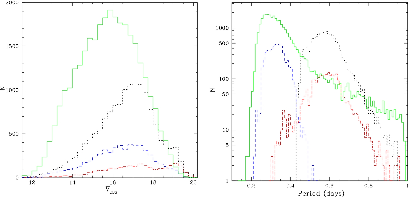
Figure 44. Light curves of two serendipitously discovered cataclysmic variables.
Download figure:
Standard image High-resolution image
Table 9. Parameters of Newly Discovered CVs
| CRTS ID | R.A. | Decl. (J2000) |  |
u | g | r | i | z |
|---|---|---|---|---|---|---|---|---|
| CSS_J003304.0+380105 | 00:33:04.09 | +38:01:05.8 | 17.8 | 20.5 | 20.5 | 20.6 | 20.5 | 19.8 |
| CSS_J004024.1+334131 | 00:40:24.18 | +33:41:31.9 | 18.3 | 20.4 | 19.0 | 18.4 | 18.1 | 18.0a |
| CSS_J031245.8+304246 | 03:12:45.82 | +30:42:46.9 | 17.2 | ... | ... | ... | ... | ... |
| CSS_J033104.4+172540 | 03:31:04.41 | +17:25:40.7 | 17.9 | 19.3 | 19.4 | 19.0 | 18.6 | 18.3 |
| CSS_J035318.1−034846 | 03:53:18.19 | −03:48:46.8 | 17.2 | ... | ... | ... | ... | ... |
| CSS_J035806.6+340343 | 03:58:06.69 | +34:03:43.8 | 16.7 | ... | ... | ... | ... | ... |
| CSS_J035905.8+175034 | 03:59:05.89 | +17:50:34.7 | 17.4 | 16.9 | 16.6 | 16.7 | 16.8 | 16.8 |
| CSS_J041138.6+232219 | 04:11:38.60 | +23:22:19.9 | 17.8 | ... | ... | ... | ... | ... |
| CSS_J042933.6+312927 | 04:29:33.65 | +31:29:27.7 | 18.3 | ... | ... | ... | ... | ... |
| CSS_J043019.9+095318 | 04:30:19.98 | +09:53:18.2 | 18.2 | 18.6 | 18.8 | 18.5 | 18.2 | 18.0 |
| CSS_J050236.5+134916 | 05:02:36.58 | +13:49:16.9 | 17.4 | 18.4 | 17.6 | 16.2 | 15.1 | 14.5a |
| CSS_J050253.1+171041 | 05:02:53.10 | +17:10:41.5 | 17.9 | ... | ... | ... | ... | ... |
| CSS_J075311.6+352631 | 07:53:11.61 | +35:26:31.4 | 16.9 | 16.9 | 16.4 | 16.2 | 16.0 | 16.0 |
| CSS_J082925.3−001351 | 08:29:25.37 | −00:13:51.0 | 16.9 | ... | ... | ... | ... | ... |
| CSS_J101233.9+074644 | 10:12:33.92 | +07:46:44.5 | 16.9 | 15.6 | 15.4 | 15.8 | 15.9 | 16.1 |
| CSS_J134504.3+004253 | 13:45:04.32 | +00:42:53.1 | 14.4 | ... | ... | ... | ... | ... |
| CSS_J152351.2+083606 | 15:23:51.22 | +08:36:06.9 | 18.7 | 14.7 | 14.7 | 15.4 | 14.4 | 14.0 |
| CSS_J164825.6+142411 | 16:48:25.62 | +14:24:11.3 | 18.0 | 21.9 | 19.8 | 18.6 | 18.1 | 17.9a |
| CSS_J172951.6+220807 | 17:29:51.64 | +22:08:07.2 | 17.1 | ... | ... | ... | ... | ... |
| CSS_J180222.4+455245 | 18:02:22.42 | +45:52:45.3 | 17.4 | 19.5 | 19.4 | 19.3 | 19.2 | 18.9 |
| CSS_J205518.8−162640 | 20:55:18.83 | −16:26:40.6 | 17.7 | 17.1 | 17.0 | 17.2 | 17.3 | 17.3 |
| CSS_J210732.6−095659 | 21:07:32.61 | −09:56:59.1 | 17.4 | 16.9 | 16.3 | 16.5 | 16.6 | 16.7 |
| CSS_J212625.0+201946 | 21:26:25.03 | +20:19:46.4 | 16.4 | 16.5 | 16.4 | 16.6 | 16.8 | 16.9 |
| CSS_J213319.4+190155 | 21:33:19.47 | +19:01:55.0 | 16.8 | 19.0 | 17.7 | 17.0 | 16.7 | 16.5a |
| CSS_J213438.4−055319 | 21:34:38.44 | −05:53:19.2 | 18.1 | 18.3 | 18.2 | 18.3 | 18.3 | 18.3 |
| CSS_J220031.2+033430 | 22:00:31.23 | +03:34:30.4 | 18.0 | 18.3 | 18.5 | 18.3 | 18.0 | 17.9 |
| CSS_J220321.3+144606 | 22:03:21.32 | +14:46:06.9 | 17.5 | 17.5 | 17.9 | 17.7 | 17.3 | 17.6 |
Notes. Column 1: Catalina ID. Columns 2 and 3: right ascension and declination. Column 4: average CSS magnitude. Columns 5–9: The SDSS-DR10 photometric magnitudes. aSystem exhibiting color excess.
Download table as: ASCIITypeset image