


ABSTRACT
The radial velocity (RV) technique is one of the most efficient ways of detecting exoplanets. However, large RV jitters induced by starspots on an active star can inhibit detection of any exoplanet present or even lead to a false positive detection. This paper presents a new multi-band RV technique capable of substantially reducing starspot-induced RV jitters from stellar RV measurements to allow efficient and accurate extraction of RV signals caused by exoplanets. It takes full advantage of the correlation of RV jitters at different spectral bands and the independence of exoplanet signals at the corresponding bands. Simulations with a single-spot model and a multi-spot model have been conducted to investigate the RV jitter reduction capability of this method. The results show that this method can reduce the RV jitter amplitude by at least an order of magnitude, allowing detection of weaker exoplanet signals without significantly increasing RV observation time and cadence. This method can greatly reduce the observation time required to detect Earth-like planets around solar type stars with ∼0.1 m s−1 long term Doppler precision if spot-induced jitter is the dominant astrophysical noise source for RV measurements. This method can work efficiently for RV jitter removal if: (1) all the spots on a target star have approximately the same temperature during RV observations; (2) the RV jitter amplitude changes with wavelength, i.e., the RV jitter amplitude ratio, α, between two different spectral bands is not close to one; (3) the spot-induced RV jitter dominates the RV measurement error.
Export citation and abstract BibTeX RIS
1. INTRODUCTION
Ever since the first exoplanet was discovered around a solar type star (51 Peg) (Mayor & Queloz 1995), high-precision radial velocity (RV) observation has become one of the most profitable methods in detecting and characterizing exoplanets. To date, more than 600 exoplanets have been discovered using the RV method. Statistics of various properties of planets have been well cataloged (Butler et al. 2006). Most of the planet-bearing stars are old and inactive, due to selection effects. For example, Jenkins et al. (2006) derived activity indices for 225 F6-M5 type stars in the southern sky and found that the jitter levels of all 21 exoplanet-host stars in their sample are very low. Martinez-Arnaiz et al. (2010) found similar results in their study. They compiled activity indices for a sample of 371 stars, and found that 17 stars in their sample are confirmed to have exoplanets. These 17 stars are either inactive or have low activity. This is because when stars are young and/or have fast differential rotation velocities, their strong dynamos can generate strong activities in their stellar photospheres, which manifest visually in the form of dark spots. The large RV jitters induced by starspots on such active stars can inhibit exoplanet detection or even lead to false positive detections. For instance, Queloz et al. (2001) found that the RV variation of a G0V star, HD 166435, is not due to the presence of an exoplanet, but rather, the surface spot activity. Henry et al. (2002) found that a Jupiter-like exoplanet signal around HD 192263 is actually caused by rotational modulation of the surface activity. Recently, Huélamo et al. (2008) and Huerta et al. (2008) have also found that two previously claimed exoplanet RV signals are actually produced by starspots on stellar surface. Mahmud et al. (2011) have shown that the presence of cool surface spots can cause the periodic RV variability of a T Tauri star, Hubble I 4.
To understand how starspot activity affects exoplanet detection using the RV technique, Saar & Donahue (1997) have made the first systematic investigation into RV variations induced by starspot activity on cool stars. In their paper, they used a single black starspot (T = 0 K) rotating on the stellar equator to derive an analytical formula to represent the relation of RV jitter to the starspot coverage fraction on the stellar surface (the filling factor) and the projected rotational velocity, vsin i. Saar et al. (1998) show that the RV variations of cool stars without exoplanets can be explained by starspot activity and non-uniform convective flows. Hatzes (2002) used a similar model to that used by Saar & Donahue (1997), except assuming a fixed spot size and placing spots randomly on the stellar surface. They found a correlation between RV jitter and spot activity similar to that from Saar & Donahue (1997). Paulson et al. (2004) made a survey of stars in a young star cluster, the Hyades (790 Myr), to search for planetary companions. They found that activity-induced jitter is consistent with the empirical relationship between activity and RV described by Saar & Donahue (1997). Desort et al. (2007) have computed the first grid of RV jitter amplitude induced by starspots for F-K type stars with different stellar and spot properties. They show that starspots with typical sizes of 1% of the stellar disk diameter in G-K type stars can mimic both the RV curves and the bisector behavior of short-period giant planets. They found that there is a weak dependence of the jitter amplitude on wavelength and proposed that such a chromatic dependence may help to distinguish planet signals from stellar spots because there is no chromatic dependence for a planet. Reiners et al. (2010) have made simulations showing that the RV jitter induced by starspots is different in different observation bands. The rms jitter level decreases from the optical to the infrared bands. This is because (1) the limb-darkening effect is different in different observational bands and (2) a starspot has a lower temperature than that of the star, hence the flux ratio between the starspot and the stellar surface increases from optical to infrared. They suggested that simultaneous observations at optical and NIR wavelengths can provide strong constraints on spot properties in active stars. Makarov et al. (2009) have further developed the starspot model used in Saar & Donahue (1997) and derived an analytical expression for RV jitter caused by a single rotating starspot with a more realistic model than before. Barnes et al. (2011) simulated RVs for M dwarfs that exhibit different starspot activity levels and determined detection thresholds for earth-mass planets in habitable zones. They found, not surprisingly, that high rotational velocities and spot activities can reduce detection sensitivity while increasing the need for more RV data points to detect exoplanets.
Since spot-induced jitter reduces exoplanet detection sensitivity, efforts have been taken by several research groups to understand the properties of jitter, and to look for an efficient way to reduce its effect on RV planet detection. Saar & Fischer (2000) found that ∼30% stars in the Lick planetary survey have significant correlations between simultaneously measured RVs and magnetic activity indices (as measured in an emission index from Ca ii λ8662). By removing this linear trend between RV and activity index, they managed to reduce dispersion in their RV measurements by an average of 17%. Santos et al. (2000) and Wright (2005) found similar results in the Geneva extra-solar planet search program and the California and Carnegie Planet Search at Keck Observatory, respectively. Melo et al. (2007) found that the RV residuals of HD 102195 (9.5 m s−1) with the planet signal removed are much higher than photon errors of their RV observations, which is largely attributed to stellar activity (see also Ge et al. 2006). They used bisectors of the HARPS cross-correlation function to correct the noise introduced by stellar activity. By subtracting a linear function, a × BIS + b, from the RV data points (where BIS is the bisector), they succeeded in reducing the residuals to 6.1 m s−1. Boisse et al. (2009) have also used this method in their observations of HD 189733 to reduce the residuals of their Keplerian orbit fit from 9.1 m s−1 to 3.7 m s−1 and obtained a more precise estimate of their exoplanet's mass. Dumusque et al. (2011a) found a correlation between the slope of the RV-activity index correlation and the effective temperature of dwarfs. They suggested that this relation can be used to correct RV jitter if the activity index and the effective temperature of the star can be provided. Recently, Boisse et al. (2011) have simulated dark spots on a rotating stellar photosphere to investigate RV jitter induced by these spots. They found that RV jitter can cause signals at the rotational period, Prot, of the star and its first two harmonics, Prot/2 and Prot/3, in the Lomb–Scargle periodograms. They use three sinusoids with periods set at these three periods to account for RV jitter induced by starspots. They have successfully removed RV jitter in four known active planet-host stars: HD 189733, GJ 674, CoRoT-7, and ι Hor using this method. Dumusque et al. (2011b) discussed the important role played by observational strategies in averaging out the RV signature of stellar noise. By choosing the observation strategy carefully, they can possibly avoid the influence of RV jitter on detection of Earth-like planets. Mahmud et al. (2011) have combined infrared and optical RV observations to show that the periodic RV variability on a T Tauri star is caused by starspots. They suggested that simultaneous RV observations in multiple wavelengths can be a powerful tool to identify starspot-induced RV jitter.
In this paper, a new multi-band RV method is presented to reduce starspot-induced RV jitter when searching for exoplanets. This method is based on the fact that starspot-induced RV jitter has a different amplitude at different observation bands. Our method is described in Section 2 and simulations used to test this method are reported in Section 3. Our discussions and conclusions are summarized in Section 4.
2. THE MULTI-BAND RV TECHNIQUE
In the proposed multi-band technique for RV data analysis, the observed stellar spectra are divided into two parts, denoted as Band A and Band B, where Band A is in the blue part of the spectrum and band B is in the red part. Band A spectra and Band B spectra are used to measure RVs, VA, i and VB, i, respectively. Here, i corresponds to an observation time ti. If the measured RVs contain both an exoplanet RV signal (Vexo, i) and starspot RV jitters at Band A and Band B, σA, i and σB, i, respectively, VA, i = Vexo, i + σA, i and VB, i = Vexo, i + σB, i, then
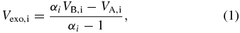
where αi = σA, i/σB, i is unknown. The physical meaning of αi is the ratio of the amplitude of RV jitters caused by starspots in the A and B bands at observation time ti. If all the starspots have similar temperatures in the same star, then αi is expected to be approximately constant (Reiners et al. 2010; Barnes et al. 2011). We assume αi as a constant α in our calculation. If α is known, then the RV signal of the planet can be derived using Equation (1). The next step is to determine the value of α. In our study, a grid of α from 1.2 to 10 is searched for the most optimal value. For a given α in the grid, Vexo, i is calculated according to Equation (1) and fitted with a Keplerian orbit. The α value which gives the most reasonable Keplerian orbit fit (by minimizing the χ2) will be adopted as an optimal α. With this optimal α and Equation (1), the jitter-free RVs of the star induced by the exoplanet can be extracted. In practice, α can be found from starspot simulations (see Reiners et al. 2010; B. Ma & J. Ge 2012, in preparation) to check if the optimal α is consistent with the reasonable starspot model. Figure 1 shows a sketch to illustrate the principle of this method.
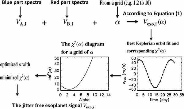
Figure 1. Sketch of the multi-band RV method principle described in Section 2. First, we derive the radial velocity VA, i and V-B, i from the red and blue parts of the spectra, respectively. Then, we use Equation (1) and assume α to derive the exoplanet signal and its Keplerian orbit. Search for a grid of α to minimize the chi-square of the Keplerian orbit fitting. At last using this optimized α to derive Vexo, i, the jitter free exoplanet radial velocity. See the the text for more information.
Download figure:
Standard image High-resolution image3. SIMULATION TESTS
A simple toy model with only one spot and a more complicated model with multi-spots have been built to test the multi-band method and show how the method works with simulated RV observation data. Only RV shifts produced by exoplanets and RV jitter caused by starspots are considered in our simulations. Therefore, the total number of RV data points chosen in the simulations required for the method demonstration is generally relatively small. However, for real RV observations, more data points are probably required for an efficient removal of starspot-induced RV jitter, since real data contain additional RV noise sources.
3.1. Spectrum Synthesis
We use the high resolution spectral library generated by Coelho et al. (2005) to synthesize our stellar template. The synthetic stellar spectrum has 0.002 nm sampling, corresponding to an intrinsic spectral resolution of R ∼ 3,000,000 in the visible wavelengths.
First, the spherical stellar photosphere is sampled into a 50×50 grid of equal-area cells, and we compute the spectrum of each individual cell as follows. For cells covered by spots, we start with a synthetic stellar spectrum with the spot temperature; we assume this is a reasonable approximation to the true spot spectrum. For cells not covered by spots, we use a synthetic stellar spectrum with the stellar effective temperature. Each cell's spectrum is then Doppler shifted according to the projected rotational velocity of the cell.
The stellar spectrum output by the program is the sum of contributions from all grid cells (Huélamo et al. 2008; Reiners et al. 2010; B. Ma & J. Ge 2012, in preparation). When we sum contributions from all the grid cells, cell spectral flux contributions are weighted by attenuated blackbody radiation spectra following the limb-darkening law. The limb-darkening coefficients are obtained from Cox (2000).
The resulting spectrum is convolved with a Gaussian line spread function corresponding to the spectral resolution of a spectrograph to be used for RV measurements. In our simulations, we choose a spectrograph resolution of R = 60, 000 at λ = 550 nm. Each resolution element of the spectrum is sampled with four pixels. We choose a simulated spectral range of 400–600 nm.
The RVs are derived by cross-correlating the spectrum of the star including the spot model against the spectrum of the star without including any spots. The cross-correlation is performed separately in Band A (400–500 nm) and Band B (500–600 nm). The RV precision is calculated according to the simulation results of Wang & Ge (2011).
3.2. Models with a Single Spot
In the simple toy model of a single starspot, the spot model is like that of Saar & Donahue (1997). The spot is at the equator of a star, with its size 10% of the stellar disk diameter. A solar-type star spectrum with Teff = 5750 K, log (g) = 4.5, and [Fe/H] = 0 is used as a spectral template of the planet hosting star, which corresponds to a G type star. The spot temperature is chosen to be 500 K lower than that of the star (Solanki 2003). The star's rotational velocity is chosen to be 5 km s−1, with its rotational period fixed at 10 days. The exoplanet's orbital period and velocity semi-amplitude are chosen to be 50 days and 50 m s−1, respectively, which corresponds approximately to a ∼1MJupiter planet. All simulations were started with a 70° initial phase difference between the exoplanet and the spot. The stellar surface is integrated with the spot to get the synthesized spectra of the star and starspot using the method described above. We choose signal-to-noise ratio S/N = 150 at 600 nm in our simulation. We have generated 10 spectra in this simulation, which is close to the minimum number of RV points required to find the input exoplanet signal. The radial velocities are derived using the cross correlation method in Band A and Band B, respectively. According to Wang & Ge (2011), the RV errors derived from Band A and Band B are 0.9 m s−1 and 1.2 m s−1, respectively.
After RVs are derived, the multi-band method technique described in Section 2 is applied to extract the exoplanet signal mixed with spot-induced jitter. Table 1 lists simulated RVs in band A (VA, i), Band B (VB, i) and the input RVs (Vinput, i). The best-fit RVs, Vi, from our multi-band technique are also included in this table. The parameter α is found to be 2.06. The errors of these RVs are assumed to be 1 m s−1, which is comparable to the precision achieved by HARPS (e.g., Mayor et al. 2003). Figure 2 shows the Lomb–Scargle periodograms and best-fit Keplerian orbit solutions of VA, i, VB, i, and Vi. Before the multi-band technique is used, the Lomb–Scargle (L-S) periodograms show that the starspot-induced jitter has prohibited detection of the exoplanet signal. After the multi-band technique is applied, the RV jitter is greatly reduced (to less than 5 m s−1) and the RV signals from the exoplanet become the dominant component in the RV residuals. The peak of the power in the L-S diagram associated with the exoplanet signal increases from ∼16 to ∼180. The best-fitting result is an exoplanet with a period of 50.8 days and semi-amplitude of 54.1 m s−1, which have ∼10% errors when comparing to the inputs. The planet signal is successfully extracted from the jitter-dominated RV data with only 10 high-precision (∼1 m s−1) RV measurements.
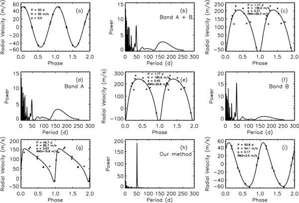
Figure 2. Plots of simulations to demonstrate the ability of the multi-band RV technique in finding a planet with an orbital period of P = 50 days and a semi-amplitude of K = 50 m s−1 around a single-spot covered star (see the text for details of this simulation). The input planet RV signal of this simulation is shown in panel (a). Also shown are the Lomb–Scargle periodograms and the best Keplerian orbit fit of the RVs obtained in Band A+B (panels (b) and (c)), Band A (panels (d) and (e)), Band B (panels (f) and (g)), and our multi-band method (panels (h) and (i)). The error bars of the derived RVs are also shown in the plot, although they are usually smaller than the symbol size.
Download figure:
Standard image High-resolution imageTable 1. Simulated Stellar RVs in Bands A and B Using a One-spot Model, and the Multi-band Technique's Best-fit RVs, Vi, in Units of m s−1
| Date (days) | VA, i | VB, i | Vi | Vinput, ia |
|---|---|---|---|---|
| 28.33 | −38 | −13 | 11.8 | 7.4 |
| 91.03 | 250 | 152 | 55.9 | 49.3 |
| 102.48 | 207 | 101 | −4.8 | −2.1 |
| 111.13 | 153 | 57 | −37.9 | −45.2 |
| 142.04 | 269 | 159 | 50.7 | 47.8 |
| 161.42 | 157 | 59 | −37.7 | −45.9 |
| 229.17 | 182 | 94 | 7.2 | 12.5 |
| 252.05 | 222 | 112 | 3.2 | 0.6 |
| 269.49 | 169 | 62 | −44.8 | −41.1 |
| 282.44 | 243 | 134 | 26.0 | 30.8 |
Note. aVinput, i is the input RV for the simulated star, for an exoplanet with a period of 50 days and a velocity semi-amplitude of 50 m s−1.
Download table as: ASCIITypeset image
3.3. Models with Multiple Spots with Solar-like Distribution
This new multi-band technique can not only largely remove RV jitter caused by a single starspot, but also by multiple spots. In the simulation of multiple spots, historical sunspot records are referenced to create a realistic distribution of multiple spots on the stellar surface, although historical sunspot sizes are small due to the inactive nature of the Sun. In order to simulate spectral characteristics with an active solar type star, each spot size in the sunspot distribution has been increased by 100 times. The choice of 100 times larger spot size causes RV jitter with an amplitude comparable to the 50 m s−1 exoplanet RV signal.
The same spectral template of the planet hosting star with the same stellar rotational velocity, period, and spot temperature as that used in the single spot modeling is adopted in this simulation. Fifteen spectra with R = 60, 000, and S/N = 150 at 600 nm, have been computed. The same cross-correlation method as used in the single spot modeling is used to extract RVs in Band A and Band B, respectively. The starspot distributions over different observation epochs in our simulation are chosen as the sunspot distributions of 15 random dates from the year 1999 in the USAF/NOAA sunspot database (http://solarscience.msfc.nasa.gov/greenwch.shtml). Based on our extensive simulations, 15 is nearly the minimal number of RV measurements needed to successfully extract the RV signals of the simulated exoplanet with a semi-amplitude of 50 m s−1 when using our multi-band technique. Table 2 shows the simulated RV data, together with the best-fit RVs derived from the multi-band method. Observation dates shown in Table 2 are JD − 2451180, where JD − 2451180 corresponds to the first day in 1999. Figure 3 shows Lomb–Scargle periodograms of these simulated RV data together with their best-fit Keplerian orbit solutions. The best-fit value of α is 2.02. The peak of the power of the 50-d exoplanet signal in the Lomb–Scargle periodogram has increased from ∼8 to 1500 after adopting the multi-band technique. The simulation results show that the multi-band method can significantly reduce the RV jitter from multiple starspots allowing a clear detection of exoplanet signals with an amplitude similar to the jitter.
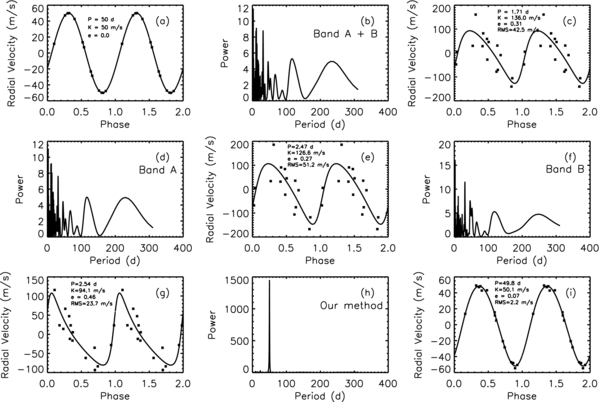
Figure 3. Plots of simulations to demonstrate the ability of the multi-band technique in finding a planet with an orbital period of P = 50 days and a semi-amplitude of K = 50 m s−1 around a multi-spot covered star (see the text for details of this simulation). The input planet RV signal of this simulation is shown in panel (a). Also shown are the Lomb–Scargle periodograms and the best Keplerian orbit fit of the RVs obtained in Band A+B (panels (b) and (c)), Band A (panels (d) and (e)), Band B (panels (f) and (g)), and our multi-band method (panels (h) and (i)). The error bars of the derived RVs are also shown in the plots, although they are usually smaller than the symbol size.
Download figure:
Standard image High-resolution imageTable 2. Simulated Stellar RVs in Bands A and B Using a Multi-spot Model, and the Multi-band Technique's Best-fit RVs, Vi, in Units of m s−1
| Date (days) | VA, i | VB, i | Vi | Vinput, ia |
|---|---|---|---|---|
| 29.0 | 33.5 | 23.5 | 13.7 | 11.5 |
| 37.0 | 45.2 | 47.2 | 49.2 | 47.2 |
| 39.0 | 185.8 | 115.8 | 47.2 | 49.8 |
| 114.0 | −75.8 | −61.8 | −48.1 | −49.8 |
| 117.0 | −117.8 | −83.8 | −50.5 | −47.8 |
| 200.0 | 31.4 | 23.4 | 15.5 | 13.4 |
| 206.0 | −167.2 | −93.2 | −20.7 | −23.2 |
| 215.0 | 84.0 | 14.0 | −54.6 | −50.0 |
| 250.0 | 35.4 | 23.4 | 11.6 | 13.4 |
| 251.0 | 5.2 | 5.2 | 5.2 | 7.2 |
| 262.0 | −23.2 | −35.2 | −47.0 | −47.2 |
| 294.0 | 90.7 | 66.7 | 43.2 | 42.7 |
| 307.0 | −4.6 | −16.6 | −28.4 | −28.6 |
| 339.0 | −106.2 | −28.2 | 48.3 | 49.8 |
| 340.0 | −68.0 | −12.0 | 42.9 | 50.0 |
Note. aVinput is the input RV for the simulated star, for an exoplanet with a period of 50 days and velocity semi-amplitude of 50 m s−1.
Download table as: ASCIITypeset image
4. DISCUSSION AND CONCLUSIONS
The multi-band RV technique is based on the fact that RV jitters induced by starspots in two different bands are correlated and the ratio of the jitters is nearly a constant. The α values from the multi-band simulations in this paper are 2.06 and 2.02, respectively, slightly depending on spot models (a single spot or multiple spots). This technique is also based on one of the important assumptions that all of the spots in one star have approximately the same temperature. Any variation of spot temperatures in active stars leads to variable αi in Equation (1), which will affect jitter reduction efficiency.
To investigate this spot temperature effect, simulations of a single spot, with a temperature assigned randomly at each epoch (5000 K, 5250 K, or 5500 K), were conducted. Three sets of Monte Carlo simulations were conducted to find the probability of success in detecting exoplanet signals with 10, 15, and 20 RV data points. Here, a successful detection is defined as a false alarm probability lower than 1% in the Lomb–Scargle periodogram. Each simulation contains 1000 trials. The resulting false alarm probability is <1% for 20 data points, ∼85% for 15 data points, and >99% for 10 data points. This result is quite different from the constant spot temperature case in Section 3.2, where a mere 10 RV points already yielded a false alarm probability <1%. Thus, varying the spot temperature randomly over time by ±250 K doubles the RV observations required to detect the exoplanet signal to a false alarm probability <1%. If we extend the starspot temperature range to 4500–5500 K, then our simulations show that the false alarm probability increases to ∼98% using 20 RV data points, and the false alarm probability would be ∼60% even when using 50 RV data points. The explanation for the degradation in successful detections is that when the spot temperature varies over a large range, the RV jitter ratio, α, between the two different bands is no longer nearly constant, and hence our assumption from Section 2 is not valid. Therefore, the proposed multi-band RV technique works most efficiently for active stars with starspots of constant temperature (within ∼500 K), and becomes less efficient when spot temperatures exhibit high variability (∼1000 K or larger).
The other important assumption for this method is that the RV jitter ratio, α, is not close to one, i.e., that the RV jitter varies across the observed wavelengths. If the RV jitter violates this assumption (one example is if the wavelength difference between two bands is very small), then because the exoplanet signal is also wavelength independent, the signals cannot be disentangled. Mathematically expressed, it is not possible to solve for Vexo, i in Equation (1) when α is equal to one. Desort et al. (2007) simulated RV jitter for FGK type stars induced by starspots with a temperature 1200 K lower than the stellar disk. They found that when they compared the 400–500 nm region to 500–600 nm, α was between 1.0 and 1.2. Reiners et al. (2010) showed that the chromatic dependence of RV jitter induced by starspots is weak if the spot temperature is far lower than the stellar surface temperature. Their simulation shows that comparing the 400–500 nm and 500–600 nm bands yields α ≫ 1 if the temperature difference between the spot and the stellar surface is lower than 1000 K. Conversely, if the temperature difference is large (>1000 K), α would be close to one and the multi-band method would not work efficiently. So, a minimal temperature difference between the spot and the disk delivers a double whammy in reducing the RV jitter: first, the smaller the temperature contrast, the more indistinguishable the spot is, and the lower the jitter amplitude becomes; second, the smaller the temperature contrast, the larger α is, and the easier it becomes to subtract off the jitter.
Reiners et al. (2010) show that the RV jitter does not decrease dramatically toward longer wavelengths (1000–1800 nm). So this multi-band method may not work efficiently if we only have near infrared band observations. However, the ratio of optical jitter to near-infrared jitter is always greater than two (Reiners et al. 2010). Thus, our multi-band RV method will work efficiently and can be a powerful tool for detecting exoplanets around active stars if both high precision optical and infrared RV measurements are combined for data analysis.
It is worth pointing out that the proposed method may provide an efficient tool for detecting an Earth-like planet around a Sun-like star using future generation ultrahigh precision Doppler instruments with precisions of ∼0.1 m s−1. This result is based on the simulation of the RV jitter of the Sun induced by sunspots using the historical sunspot record (more details on sun spot jitter simulation studies are shown in B. Ma & J. Ge 2012, in preparation). For instance, we tried simulating sunspot-induced RV jitter at 50 random dates from the sunspot record from the years 1999–2000, adopting constant sunspot temperatures, and adding the jitter to an Earth-like exoplanet signal. We generated spectra with a resolution of R = 60, 000 and signal-to-noise ratio S/N = 1500 at 600 nm, which gives us an RV precision of 0.09 m s−1 and 0.12 m s−1 in Band A and Band B, respectively. Without adding any other noise to this RV simulation, the Earth-like planet signal could be clearly detected with this ∼0.1 m s−1 precision RV data after RV jitter was removed using our multi-band method. Figure 4 shows the results of this simulation. The Lomb–Scargle periodograms in Figure 4 clearly show that the sunspot jitter overwhelms the Earth-like planet signal before the multi-band method is applied in the RV data analysis. After this multi-band method is applied, the Earth-like planet signal is clearly detected. Running ∼100 Monte Carlo iterations of the simulations demonstrates that it requires 40–50 data points to detect this Earth-like planet signal if the RV precision is 0.1 m s−1. For comparison, it requires more than ∼300 RV data points with 0.1 m s−1 precision to detect this Earth-like planet signal if the proposed multi-band method is not adopted. However, if the RV precision is changed to 1 m s−1, our method has no significant advantage over the traditional method. This is because we cannot fully utilize the correlation between spots' RV jitters across different spectral bands when the spots' jitters are buried in the photon noise of the RV measurements. Therefore, the proposed multi-band RV method can improve the sensitivity of exoplanet detection and Keplerian orbit fitting only when starspot jitter dominates the error bars of RV measurements.
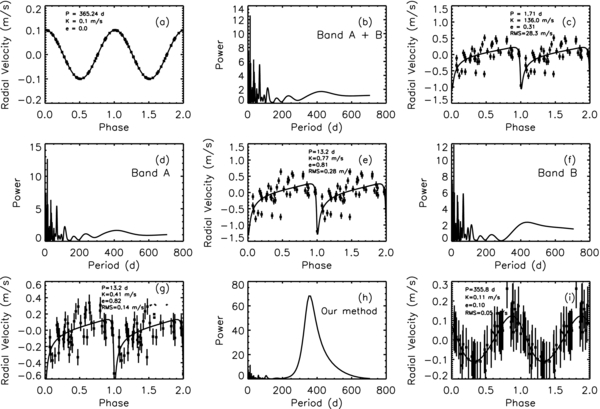
Figure 4. Plots of simulations to demonstrate the ability of the multi-band technique in finding an Earth-like planet with P = 365.24 days and K = 0.1 m s−1 around a Sun-like star using 0.1 m s−1 RV precision. The input Earth-like planet RV signal of this simulation is shown in panel (a). Also shown are the Lomb–Scargle periodograms and the best Keplerian orbit fit of the RVs obtained in Band A+B (panels (b) and (c)), Band A (panels (d) and (e)), Band B (panels (f) and (g)), and our multi-band method (panels (h) and (i)). The error bars of the derived RVs are also shown in the plots.
Download figure:
Standard image High-resolution imageWe have also studied whether the multi-band RV method will work in narrower wavelength regions than in Section 3.1. We chose 490–550 nm and 550–620 nm: a popular range of observed wavelengths among authors that use iodine cells as wavelength calibration sources. Simulations similar to those in Sections 3.2 and 3.3 were conducted using these two bands, and the results showed that the multi-band technique worked nearly as efficiently as in Sections 3.2 and 3.3. Therefore, our method, in principle, can be applied to small wavelength bands. However, in reality, it is not practical to use infinitely small observation bands, since the error bar would increase if the observation band included hardly any stellar lines from which to measure RVs.
In Figure 5, we present a flow chart on how to use this multi-band method in an RV analysis. First, RVs are measured in two different wavelength bands. If the two band RV signals are not consistent with each other in the measurements, then there may be wavelength-dependent jitter in the RV data. The multi-band method will then be used to extract jitter-free RVs and do the Keplerian orbit fitting. If the two bands' RVs are consistent with each other, then either the spot-induced RV jitter ratio of the two bands is close to one or there is no jitter caused by starspots. Line bisector analysis or photometric follow-up can be used to further investigate the existence of star spots. If no evidence is found for star spots, then Keplerian orbit fitting can be conducted with the RV data to derive planet orbital parameters. If there is evidence for existence of star spots, then the multi-band analysis can be repeated, after adding new RV observations in a longer wavelength band to minimize the impact of spots on the RV measurements and also increase the jitter ratio, α, between the bands.

Figure 5. Suggested flow chart of how to use the multi-band method described in this paper to analyze the RV observations.
Download figure:
Standard image High-resolution image
In summary, a new multi-band technique is presented to reduce RV jitter induced by starspot activity when detecting exoplanets using RV observations. The simulations show that our method can significantly reduce RV jitter when the RV jitter level is at a similar level to or much greater than the exoplanet's Keplerian orbital semi-amplitude. However, three conditions are needed for this method to work efficiently: (1) all the spots in an observed star have approximately the same temperature during the RV observations; (2) the RV jitter ratio, α, between the two bands are not close to one; and (3) the spot jitter dominates the error bars of the RV measurements.
We acknowledge the support from NSF with grant NSF AST-0705139, NASA with grant NNX07AP14G (Origins), UCF-UF SRI program, DoD ARO Cooperative Agreement W9 11NF-09-2-0017, Dharma Endowment Foundation and the University of Florida. Bo Ma thanks the University of Florida for providing a Graduate Alumni Fellowship. We thank Dr. Brian L. Lee for proofreading the paper, which helped to improve this paper's quality. We also thank the referee for constructive suggestions which improved this paper's quality.