


ABSTRACT
We investigate the spatial density configuration of stars around four metal-poor globular clusters (NGC 6266, NGC 6626, NGC 6642, and NGC 6723) in the Galactic bulge region using wide-field deep J, H, and K imaging data obtained with the Wide Field Camera near-infrared array on the United Kingdom Infrared Telescope. A statistical weighted filtering algorithm for the stars on the color–magnitude diagram is applied in order to sort cluster member candidates from the field star contamination. In two-dimensional isodensity contour maps of the clusters, we find that all four of the globular clusters exhibit strong evidence of tidally stripped stellar features beyond the tidal radius in the form of tidal tails or small density lobes/chunks. The orientations of the extended stellar substructures are likely to be associated with the effect of dynamic interaction with the Galaxy and the clusterʼs space motion. The observed radial density profiles of the four globular clusters also describe the extended substructures; they depart from theoretical King and Wilson models and have an overdensity feature with a break in the slope of the profile at the outer region of clusters. The observed results could imply that four globular clusters in the Galactic bulge region have experienced strong environmental effects such as tidal forces or bulge/disk shocks of the Galaxy during the dynamical evolution of globular clusters. These observational results provide further details which add to our understanding of the evolution of clusters in the Galactic bulge region as well as the formation of the Galaxy.
Export citation and abstract BibTeX RIS
1. INTRODUCTION
According to modern cold dark matter cosmology, galaxies are hierarchically assembled by the merging or accretion of small fragments (Baugh et al. 1996; Klypin et al. 1999; Moore et al. 1999; Diemand et al. 2007). In this theory, the stellar halos of galaxies such as the Milky Way are mostly built up from small substructures such as satellite galaxies (Searle & Zinn 1978; Johnston 1998; Bullock et al. 2001; Abadi et al. 2006; Font et al. 2006; Moore et al. 2006). These satellite systems suffer significant tidal disruption and mass loss as a reult of tidal forces and shocks that take place in their host galaxies during the process of accretion, thereby producing a number of stellar substructures such as tidal tails or streams in the galactic halo (Bullock & Johnston 2005). Thus, the study of stellar streams in the Milky Way is valuable for reconstructing the accretion history of the Galaxy (Law et al. 2009; Koposov et al. 2010) and for understanding the potential of the Galaxy (Odenkirchen et al. 2009).
In the last two decades, numerous stellar streams and tidal tails have been discovered in the Galactic halo. The Sagittarius dwarf galaxy and its stellar streams (Ibata et al. 1994, 1995, 1997, 2001; Vivas et al. 2001; Majewski et al. 2003; Newberg et al. 2003; Martínez-Delgado et al. 2004; Belokurov et al. 2006a) are the most well studied out of the many other recently discovered stellar streams (Helmi et al. 1999; Ivezić et al. 2000; Yanny et al. 2000, 2003; Newberg et al. 2002; Martin et al. 2004; Rocha-Pinto et al. 2004; Martínez-Delgado et al. 2005; Duffau et al. 2006; Grillmair 2006; Jurić et al. 2008). Sky survey projects, such as the Sloan Digital Sky Survey and 2MASS, are discovering more stellar substructures in the Galactic halo; newly discovered stellar streams include the Virgo stellar stream (Vivas & Zinn 2006; Vivas et al. 2008), the Orphan Stream (Grillmair 2006; Zucker et al. 2006; Belokurov et al. 2007), and the Cetus stream (Newberg et al. 2009; Koposov et al. 2012). More recent works have reported that some of these streams are associated with globular clusters (Drake et al. 2013; Grillmair et al. 2013).
Globular clusters have been one of the most investigated types of stellar systems. They have provided crucial information about the formation and evolutionary mechanisms of the Galaxy. However, recent photometric and spectroscopic studies have further amended the accepted view of how globular clusters formed and their contribution to the formation of the Milky Way. It appears that they are not just simple stellar populations as was previously thought (Gratton et al. 2004; Carretta et al. 2009), and some of them, such as ω Centauri (Lee et al. 1999) and NGC 6656 (Lee et al. 2009), are even considered to be surviving remnants of the first building block that merged into the Milky Way. Several globular clusters in the Milky Way (about 27% of the Milky Wayʼs globular clusters; Mackey & Gilmore 2004) could have formed via accretion or the merging of more complex systems. In addition, recent work suggests that globular clusters were 8–25 times more massive when they first formed than they are at present (Conroy et al. 2011; Schaerer & Charbonnel 2011). Thus, the stellar streams around globular clusters are important objects to study to further our understanding of the merging or accretion history of the Milky Way and to gather information regarding the dynamical evolution of globular clusters. Indeed, the remarkable long tidal tail of Palomar 5 (Odenkirchen et al. 2001; Grillmair & Dionatos 2006a) and NGC 5466 (Belokurov et al. 2006b; Grillmair & Johnson 2006), as well as the presumed globular cluster stream GD-1 (Grillmair & Dionatos 2006b), are spectacular examples of globular cluster streams. The tidal bridge-like features and common envelope structures around M53 and NGC 5053 (Chun et al. 2010) are also particularly interesting as they are the evidence of an accretion event of dwarf galaxies into the Milky Way. Slightly extended tidal substructures also appear in the vicinity of several globular clusters (Grillmair et al. 1995; Leon et al. 2000; Sohn et al. 2003).
Despite numerous discoveries of globular cluster streams, most of the globular cluster streams found to date have been in the Galactic outer halo. However, there are more than 40 globular clusters in the Galactic bulge region, and the origin of metal-poor globular clusters in this region is still unclear. There have been few studies of the stellar streams of globular clusters in the bulge region. The stellar substructure around globular cluster NGC 6626 was the first discovery in this region (Chun et al. 2012). In a hierarchical model, it can be seen that vigorous merging events of subclumps exist in the bulge region of galaxies like the Milky Way (Katz 1992; Baugh et al. 1996; Zoccali et al. 2006). These merging events then result in a wide metallicity distribution (![$-1.5\leqslant [{\rm Fe}/{\rm H}]\lt 0.5$](https://content.cld.iop.org/journals/1538-3881/149/1/29/revision1/aj503563ieqn1.gif) ; McWilliam & Rich 1994; Zoccali et al. 2003) of stars in the bulge region (Nakasato & Nomoto 2003). Terzan 5 is an example of a past merging event in the bulge region (Ferraro et al. 2009). Therefore, we can expect to discover extratidal substructures around some of the globular clusters in the bulge region.
; McWilliam & Rich 1994; Zoccali et al. 2003) of stars in the bulge region (Nakasato & Nomoto 2003). Terzan 5 is an example of a past merging event in the bulge region (Ferraro et al. 2009). Therefore, we can expect to discover extratidal substructures around some of the globular clusters in the bulge region.
In this study, we investigated the spatial density distribution of stars around four metal-poor globular clusters in the Galactic bulge region—NGC 6266, NGC 6626, NGC 6642, and NGC 6723. We identified the bulge region as the area within 3 kpc of the Galactic center. Table 1 shows the basic parameters of the four globular clusters. In order to reduce the effect of high extinction toward the bulge, we used wide-field (45' × 45') near-infrared JHK photometric data obtained from an observation with the Wide Field Camera (WFCAM) array attached to the United Kingdom Infrared Telescope (UKIRT). Section 2 presents our observations, data reduction process, and photometric measurements. The statistical analysis and filtering technique used for member star selection are described in Section 3. In Section 4, we investigate two-dimensional stellar density maps and the radial profile of the clusters to trace the stellar density features. The discussion of our investigation is presented in Section 5. Lastly, we summarize the results and discussion in Section 6.
Table 1. Basic Parameter for Four Target Globular Clusters and the Position of Three Comparison Fields
| Target | α | δ | Rsun | RGC | rc | rt | [Fe/H] | Index |
|---|---|---|---|---|---|---|---|---|
| (J2000) | (J2000) | (kpc) | (kpc) | (') | (') | |||
| NGC 6266 | 17:01:12.80 | −30:06:49.4 | 6.8 | 1.7 | 0.22 | 8.97 | −1.18 | ⋯ |
| NGC 6626 | 18:24:32.81 | −24:52:11.2 | 5.5 | 2.7 | 0.24 | 11.27 | −1.32 | ⋯ |
| NGC 6642 | 18:31:54.10 | −23:28:30.7 | 8.1 | 1.7 | 0.1 | 10.07 | −1.26 | ⋯ |
| NGC 6723 | 18:59:33.15 | −36:37:56.1 | 8.7 | 2.6 | 0.83 | 10.51 | −1.10 | ⋯ |
| Comparison1 | 18:31:37.44 | −29:19:30.36 | ⋯ | ⋯ | ⋯ | ⋯ | ⋯ | NGC 6266, NGC 6642 |
| Comparison2 | 17:12:59.28 | −23:12:51.84 | ⋯ | ⋯ | ⋯ | ⋯ | ⋯ | NGC 6626 |
| Comparison3 | 19:09:22.32 | −32:55:42.96 | ⋯ | ⋯ | ⋯ | ⋯ | ⋯ | NGC 6723 |
Note. Rsun and RGC are distances from the Sun and the Galactic center, respectively. rc and rt indicate the core radius and tidal radius. The basic parameter information is from the catalog Harris (1996; 2010 edition). Index indicates the globular clusters to which comparison fields were applied in the C–M mask filtering and optimal contrast filtering techniques.
Download table as: ASCIITypeset image
2. OBSERVATION, DATA REDUCTION, AND PHOTOMETRY
Photometric imaging data for four globular clusters were observed using the WFCAM on the 3.8 m UKIRT in Hawaii in 2010 April and July. The WFCAM is an infrared mosaic detector of four Rockwell Hawaii-II (HgCdTe 2048 × 2048) arrays with a 12 83 gap between the arrays. Four separately pointed observations (four tiles) result in a filled-in sky area of 0.75 square degrees with a pixel scale of 04. Our target clusters were observed using the four-tile observations in three band filters (
 , and K) to get continuous sky images covering a total field-of-view of 0.75 square degrees. The individual image of each cluster for one tile was recorded in short (1 s for JHK) and long (5 s for JH, and 10 s for K) exposures to optimize the photometry of bright and faint stars. A five-point dithering pattern was applied to reject bad pixels and cosmic rays. At each dithered position, a 2 × 2 micro-stepping observation was also carried out to get well-sampled stars. A separate sky observation was obtained for removing thermal background emission after observing the target images. We also observed several comparison fields in the bulge region using the same observation strategy for observing the clusters. The stars in the comparison field area were used during the processes of the color–magnitude (C–M) mask filtering technique and the optimal contrast filtering technique in the following section in order to estimate the field star contamination around the globular clusters on the color–magnitude diagram (CMD, see Section 3). Three comparison fields were finally selected using the following condition: the comparison field was not very distant from the clusters on the sky, and the morphology of the CMD for the field stars was similar to that of the globular clusters. The coordinates of the selected comparison fields were indicated in Table 1. Table 2 provides the exposure time of each filter for the four globular clusters.
Table 2. Observation Summary of Four Globular Clusters
| Target | Filter | Exp. Time | FWHM |
|---|---|---|---|
| (micro-step × dither × second) |

|
||
| NGC 6266 | J |

|
0.78, 0.77 |
| H |

|
0.78, 0.76 | |
| K |

|
0.74, 0.77 | |
| NGC 6626 | J |

|
0.92, 0.90 |
| H |

|
0.88, 1.05 | |
| K |

|
0.91, 0.76 | |
| NGC 6642 | J |

|
0.86, 0.87 |
| H |

|
0.81, 0.79 | |
| K |

|
0.82, 0.78 | |
| NGC 6723 | J |

|
0.95, 0.99 |
| H |

|
1.07, 1.06 | |
| K |

|
0.98, 0.97 |
Download table as: ASCIITypeset image
Standard data reduction for near-infrared imaging, which includes dark subtraction, flat fielding, and the removal of crosstalk, was completed by the pipeline of the Cambridge Astronomy Survey Unit (CASU). Then thermal emission backgrounds were made by median-combining the CASU-processed images of the separate sky observations. The resulting blank sky images were subtracted from all the target images. The residual sky background level of each target image was also removed. All sky-subtracted images were interleaved into a single image for photometric analysis using Swarp (Bertin et al. 2002). The final resampled images of the four globular clusters have a wide-field area of about 45' × 45', which is sufficiently large to cover from the center of each target cluster to two times its tidal radius. The average seeing condition of stars in the resampled images is between 0.75 and 1.05 arcsec. Table 2 summarizes the average FWHM values for each filter.
Stellar photometry on each detector was performed using the point-spread function (PSF) fitting routine ALLSTAR (Stetson & Harris 1988). The PSF varying quadratically with position was first constructed with the DAOPHOT II program using 100–150 bright and isolated stars (Stetson 1987). The quality of the PSF was improved by removing neighboring faint stars then iteratively reconstructing the PSF. The instrumental magnitude of the individual stars on each array was estimated via the ALLSTAR process using the improved PSF. The raw positions of the stars on the detector were transformed into an equatorial coordinate system using the 2MASS point-source catalog. The instrumental magnitudes of the stars were transformed on to the 2MASS filter system using the color term from the WFCAM and 2MASS systems (Dye et al. 2006). Then the photometric zero points were finally computed and calibrated by comparing the magnitudes of stars common to both our photometric catalog and the 2MASS catalog. The astrometric and photometric data of each chip on a mosaic were finally combined into a whole set of data for the target cluster. Stellar objects with photometric measurements error larger than 0.1 mag were removed in order to reduce spurious detection. We also measured the individual extinction value of each star according the position of the sky by using the map of Schlegel et al. (1998). The mean E(J-K) and extinction values in K are  and AK = 0.14 for NGC 6266,
  and AK = 0.18 for NGC 6626,
  and AK = 0.15 for NGC 6642, and
  and AK = 0.08 for NGC 6723. We subtracted derived extinction values from the observed magnitude.
3. PHOTOMETRIC FILTERING FOR MEMBER STAR SELECTION
In order to accurately trace the stellar distribution around globular clusters, it is important to reduce the contamination of the field stars and to enhance the density contrast between the cluster candidate stars and the field stars. Although many statistical methods for filtering field stars have been introduced in the past few decades, the C–M mask filtering technique (Grillmair et al. 1995) and the optimal contrast filtering technique (Odenkirchen et al. 2003) have been frequently used. We also basically followed these two methods (for a detailed description, see Grillmair et al. 1995; Odenkirchen et al. 2003; Chun et al. 2012).
We first define new orthogonal color indices c1 and c2 from the one-dimensional distribution of stars in a  versus
  color–color diagram (see Figure 2 of Chun et al. 2012). The color indices were chosen in such a way that the c1 axis was placed along the main distribution of the stars, while the c2 axis was perpendicular to the c1 axis. Equation (1) shows the general forms of two orthogonal color indices, and Table 3 indicates the coefficients a and b of the new color indices for each cluster.

Table 3. The Coefficient a and b of New Color Indices For Each Cluster
| Target | a | b |
|---|---|---|
| NGC 6266 | 0.748 | 0.663 |
| NGC 6626 | 0.784 | 0.621 |
| NGC 6642 | 0.757 | 0.653 |
| NGC 6723 | 0.750 | 0.661 |
Download table as: ASCIITypeset image
In the  CMD, we rejected all stars with
  where
where  is the dispersion in c2 for stars with magnitude K. The stars within 2–5rh for each cluster were used when we defined the rejection limit. The left panel of Figure 1 shows a
  CMD for stars in 2–5rh from the cluster center. The lines indicate our rejection limit; we considered that stars outside this boundary were unlikely to be cluster member stars.

Figure 1.
 and
and  color–magnitude diagrams of stars for four globular clusters. The left panel shows the
  CMD of stars in the central region of clusters. The lines in the
  plane are the
  rejection limit at K magnitudes. The second, third, and fourth panels are the
  CMDs for the stars in the cluster central region, in the assigned comparison region, and in the total field of four clusters. The grid lines in
  CMDs indicate the filtering mask envelope where the S/Ns of cluster star counts are maximized through a C–M mask filtering technique. The stars outside the grid lines are highly unlikely to be cluster members. The optimal contrast filtering technique was also applied to this envelope.
Download figure:
Standard image High-resolution imageAfter this preselection in the  plane, we defined the locus of the cluster on the CMD where the signal-to-noise ratio (S/N) of the cluster star count was maximized in contrast to the comparison field stars using the C–M mask filtering technique in the
  plane. First, we made a representative sample of CMDs for the cluster and the fields using the stars in the central region of the cluster and the observed comparison fields. The second and third panels of Figure 1 show the
  CMDs of stars within 30–40 from each cluster center and the selected comparison region, respectively. The right panel shows the
  CMD of the stars in the total survey region for the cluster. Then, the CMDs of the cluster and comparison were subdivided into small subgrid elements, and the S/N in each subgrid element was calculated using Equation (2):

where  and
and  are the number of stars in the subgrid elements for the cluster and comparison region, respectively; g is the area ratio of the cluster region to comparison region. From array s, we computed the cumulative number of stars for the cluster Ncl(k) and comparison Nf(k), respectively, by sorting the elements of
  into a series of descending order with a one-dimensional index of k. Then, a cumulative S/N S(k) was calculated using Equation (3):

S(k) becomes a maximum value for a specific subarea of the C–M plane, and the  corresponding to the maximum value of S(k) was chosen as an optimal threshold, slim. The filtering mask area in the
  plane was then determined by selecting subgrid elements with larger
  values than the determined slim. The solid lines in the second, third, and fourth panels in Figure 1 represent the selected filtering mask envelope. The entire sample of stars in the determined filtering mask area was considered in the following filtering analysis.
Finally, we applied the optimal contrast filtering technique to the stars in the determined filtering mask envelope obtained from the C–M mask filtering technique. We calculated the number density distribution of stars in the  C–M plane (Hess diagram) for the cluster and the comparison field. The bin size of the Hess diagram is the same as that of the C–M mask filtering technique. Then, the density of cluster stars nc(k) at a given position k on the sky was derived from Equation (4):

where  and
and  are the cluster star density and the field star density in the jth subgrid in the optimal mask envelope of the C–M plane and in the kth bin in the position on the sky; fc and fF are the normalized density distribution of the cluster and the comparison field in the optimal mask envelope in the Hess diagram of
  . In the optimal contrast filtering technique, the ratio
  of the number density distribution of the cluster stars to the comparison field stars in the optimal mask envelope of
  CMD was used as a conditional weight to determine cluster membership. The number density of stars in the sky was calculated by summing up the conditional weights of all stars and dividing this sum by the factor
  . Thus, this yields the estimated number of cluster stars nc plus a term of
  , the number of contaminating field stars attenuated by a.
4. SPATIAL DENSITY FEATURES OF STARS IN THE VICINITY OF THE FOUR GLOBULAR CLUSTERS
In this section, we present the spatial density features of the stars in the vicinity of the four globular clusters. The large area of the WFCAM data (45' × 45' of the sky) enables us to examine the features of the stellar density distribution from the cluster center to a distance of at least two times the tidal radius. The two-dimensional density distribution and the radial density profile for each cluster were investigated using the selected stars via a C–M mask filtering technique and the weighted number obtained from the optimal contrast filtering technique.
Two-dimensional stellar surface density maps of the clusters were constructed using Equation (4). The sky plane of the clusters was divided into small grids with pixel widths of  , and the weighted counts of stars were calculated in those pixels. The field star contamination was then constructed by masking the central region within 1–
 and fitting a low-order bivariate polynomial model. Figure 2 shows the constructed field star contamination for each cluster, and the density gradients or variations of field stars across the globular cluster are represented with grayscale. We subtracted these field stars contamination maps and made the field across the globular cluster essentially flat. The residual background density map was also made using the same method with field star contamination maps, but in this case, we just subtracted the mean density level of the residual background density map. The star number density map of each cluster was then smoothed with a Gaussian smoothing algorithm to increase the S/N and enhance the spatial frequencies of interest. The isodensity level is described by a contour with a standard deviation unit
  of the background level on the smoothed map with various kernel values. The distribution map of the
  value for the observed region was also derived from the map of Schlegel et al. (1998) to examine possible extinction effects.

Figure 2. Field star contribution maps for four globular clusters. The density gradients and variation across the globular clusters are shown by the grayscale. The sidebar indicates the number of stars per square pixels.
Download figure:
Standard image High-resolution imageThe radial number density profiles of the globular clusters are useful for understanding the internal and outer structure of the globular clusters. This overall structure has been described by the King (1966) model, which is characterized by a truncated density profile at the outer edge. However, according to the results of a recent wide-field observation, the radial number density profiles of several globular clusters are not truncated at their outer edges; instead, they have an extended overdensity feature that departs from the behavior predicted by the King (1966) model and smoothly drops toward the background level (Grillmair et al. 1995; Leon et al. 2000; Testa et al. 2000; Rockosi et al. 2002; Lee et al. 2003; Olszewski et al. 2009; Carballo-Bello et al. 2012). Numerical simulations also reproduced and characterized this overdensity feature as a break in the slope of the radial profile due to extratidal stars around globular clusters (Combes et al. 1999; Johnston et al. 1999, 2002). In these models, the break in the slope of the radial profile was described by a power law  . The Wilson (1975) model has also been used to describe the structure of globular clusters. Indeed, McLaughlin & van der Marel (2005) fitted the Wilson model to the radial density structure of globular clusters in the Galaxy and the Magellanic Clouds. We note that the Wilson model is spatially more extended than the King model (see McLaughlin & van der Marel 2005).
We also derived the radial surface density profile of each cluster and tried to find evidence of an extratidal extension at the outer edges of the clusters. In order to construct the radial density profiles, we used concentric annuli with a width of 045 ranging from the cluster center out to a radius of 200 and then counted the weighted number of stars in each annulus. The number density of stars was then calculated by dividing the sum by the area of the annulus. The contribution of field stars on the radial profile was estimated from the field star contamination maps in Figure 2 and subtracted from the radial profile. Then the residual background density level which was measured on the residual background density map was also removed from the counts. The error on the number density was estimated by the error propagated from a Poisson statistic for star counts. We examined the radial completeness for measuring the crowding effect of the inner regions of the clusters by applying the artificial star test and then recovered the crowding effect using the radial complete ratio. However, the most central regions of the clusters were not resolved enough to derive the number density profile because of the crowding effect even though we compensated for the number density. Therefore, for the central regions, we combined our number density profiles with the previously published surface brightness profiles of Trager et al. (1995). The surface brightness profile of Trager et al. (1995) was converted into a number density scale by the equation,  , where C is an arbitrary constant to match the number density profile and surface brightness profile. Then, the final number density profiles were empirically fitted by the King model and the Wilson model. We also derived radial surface density profiles for a different direction, for which we divided an annulus into eight Sections (S1–S8), each with an angle of
  , as shown in Figure 3. The annulus widths were assigned to be
  at the innermost region with
  ,
,  at the middle region with
  and 20 at the outer region with
  . We note that some radial density points with small number statistics could not be plotted because the number densities in these regions were lower than the background density level.

Figure 3. Reseau plot used for the radial density profile. The radial surface densities were measured in concentric annuli. We divided each annulus into eight angular Sections (S1–S8) in order to derive the surface density profiles in a different direction.
Download figure:
Standard image High-resolution image4.1. NGC 6266 (M62)
The star count map around NGC 6266 and the surface density maps smoothed by a Gaussian kernel value of 0 045 and 012 are shown in Figure 4 from the top left panel to the bottom left panel. The gray density map in the bottom right panel of Figure 4 is the distribution map of E(B-V) of Schlegel et al. (1998). The contour lines indicate
  , and
, and  . The contour lines with a Gaussian kernel value of 012 are overlaid in a star count map and the E(B-V) map. The direction toward the Galactic center and the direction perpendicular to the Galactic plane are indicated as solid and dashed lines, respectively. The proper motion of NGC 6266, i.e.,
  and
and  (Dinescu et al. 2003), is indicated by a long arrow. The circle in each panel is the tidal radius of
  (Harris 1996).

Figure 4. From top left to bottom right, the star count map around NGC 6266, the surface density maps smoothed by Gaussian kernel values of 0045 and 012, overlaid with isodensity contour levels  and
and  , and the distribution map of E(B-V). The circle indicates the tidal radius of NGC 6266, the arrow represents the proper motion of the cluster, the solid line indicates the direction of the Galactic center, and the dashed line shows the direction perpendicular to the Galactic plane.
Download figure:
Standard image High-resolution imageFigure 4 clearly shows overdensity substructures around NGC 6266 that extend toward the east and northwest to  at levels larger than
  . The stellar substructure in the east direction lies along the direction of the Galactic center and the direction opposite of the proper motion. In addition, the extended structure to the northwest is likely aligned with the perpendicular direction opposite to the Galactic plane, and its marginal extension seems to bend toward the direction of proper motion. We note that the density feature at the southern region of the cluster is likely to be affected by the dust extinction as shown in the bottom right panel of Figure 4.
In the upper panel of Figure 5, the radial surface density profile of NGC 6266 is plotted, along with the King model and the Wilson model, which are arbitrarily normalized to our measurements. In the central region of the cluster, we replaced the number density profile with the surface brightness of Trager et al. (1995). The profile of Trager et al. (1995) connects smoothly with our number density profile at a radius of  . However, the number density profile shows an overdensity feature that departs from the King model and the profile of Trager et al. (1995), with a break in the slope at a radius of log(
 ) ∼ 0.65 (
 ). Here, we note that the profile of Trager et al. (1995) in the outer region might suffer from background contamination and bias toward bright stars (see Chun et al. 2012; Noyola & Gebhardt 2006), while our number density profile in this study has no bias due to bright stars. The overdensity feature seems to extend to a radius of log(
 ) ∼ 1.15 (
 ). The Wilson model shows a more extended profile toward the outer region and seems to fit better with our measurements than the King model. The excess density at this radial distance resembles a radial power law with a slope of
  , which is steeper than the case of
  predicted for a constant mass-loss rate over a long time (Johnston et al. 1999). Thus, the overdensity feature at the outer region of NGC 6266 is indeed evidence of the extended substructures shown in Figure 4.

Figure 5. Upper: radial surface density profile of NGC 6266 with the theoretical King model (solid curve) and the Wilson model (dotted curve). In the central region, we plot the surface brightness profile (Trager et al. 1995) as open squares. The arrow indicates the tidal radius ( ) of NGC 6266. The overdensity feature at the region of
  was described by a power law, i.e., a straight line in logarithmic scale with a slope of
  . The mean number density of stars in the overdensity region is estimated as
  per square arcmin. Lower: radial surface density profiles of eight different angular Sections (S1–S8). The other notations are the same as those of the radial surface density profile in the upper panel.
Download figure:
Standard image High-resolution imageThe lower panel of Figure 5 shows the radial surface number density profiles for eight angular sections with a different direction as shown in Figure 3. We note that some of the radial density points in Sections 5–8 were not presented because the number densities in these regions were lower than the subtracted residual background level. The radial profiles in Sections 1–4 show the overdensity features at a radius of  . The overdensity features in Sections 1, 3, and 4 seem to extend to more distant radii than
  . The mean surface densities (μ) in these sections are particularly higher than the total average density and those in the other sections. In addition, the slopes of the profiles in Sections 1 and 4 are shallower than the mean slope of the profile and those of other angular sections. The mean density levels and shallow slopes in these sections are in good agreement with the extended stellar substructures in the direction of the Galactic center, in the direction opposite to the proper motion, and in the opposite direction perpendicular to the Galactic plane. On the other hand, the overdensity features do not appear in Sections 5–7 where prominent stellar substructures were not shown in the two-dimensional contour map. The mean densities without overdensity features were also somewhat lower than the total average density.
4.2. NGC 6626 (M28)
The top left to bottom right panels of Figure 6 show the star count map of NGC 6626, the isodensity contour map smoothed by a Gaussian kernel value of 0045 and 012, and the distribution of the E(B-V) extinction value of Schlegel et al. (1998). The isodensity contour lines correspond to the level of  , and
, and  . The proper motion of
  and
and  (Casetti-Dinescu et al. 2013) is represented by a long arrow. The dashed line and solid line indicate the direction of the Galactic center and the perpendicular direction of the Galactic plane, respectively. The tidal radius of NGC 6626 (i.e.,
  ) from Harris (1996) is also plotted as a circle.

Figure 6. Star count map around NGC 6626, the surface density contour maps smoothed by Gaussian kernel values of  and
and  , and the distribution map of E(B-V) of Schlegel et al. (1998) are plotted from the top left to the bottom right panels. The contour levels indicate
  and
and  . The long arrow indicates the proper motion of the cluster. The different lines indicate the direction of the Galactic center (solid line) and the direction perpendicular to the Galactic plane (dashed line). The circle indicates the tidal radius of NGC 6626.
Download figure:
Standard image High-resolution imageIn Figure 6, it is apparent that the stellar density distribution around NGC 6626 shows distorted overdensity features and extended tidal tails beyond the tidal radius. The tidal tails seem to stretch out symmetrically to both sides of the cluster, extending toward the east and west directions from the cluster center to a radial distance of  . In addition, the two tidal tails are likely to be aligned with the directions of the Galactic center and anti-center. Although there are no apparent features extending toward the direction of the proper motion in the surface density maps, there is a clumpy substructure in the northern area, which is aligned with the direction opposite to the proper motion. Chun et al. (2012) first found the prominent overdensity feature that extends toward the direction perpendicular to the Galactic plane within the tidal radius of NGC 6626. We also found a stellar substructure similar to that found by Chun et al. (2012) in the contour map with a kernel value of 0045. This substructure extends toward the northwest direction within the tidal radius but is not as prominent as the substructure observed by Chun et al. (2012). We note here that our spatial density distribution has a wider field of view than that of Chun et al. (2012), which has enabled us to estimate and calibrate the underlying background substructure more accurately. Thus, the stellar density structure in this study is more homogeneous and less affected by field star contamination.
A radial surface density profile for NGC 6626 was presented in the upper panel of Figure 7. In the central region of the cluster, the number density profile was substituted with the surface brightness profile of Trager et al. (1995), which connects to the number density profile at the middle range. The theoretical King model and the Wilson model were also plotted to characterize the observed radial profile. It is apparent that our number density profile does not trace the King model and the Wilson model at the outer region of the cluster; instead, it shows an overdensity feature with a break in the slope of the profile at a radius of log( ) ∼ 0.5
  . The overdensity feature extends out to log(
 ) ∼ 1.1
  , and the profile in this region is characterized by a power law with a slope of
  . This slope is not very different from the slope of
  , predicted for a constant mass-loss rate over a long time (Johnston et al. 1999). The overdensity feature in the radial profile is indicative of extended tidal tails and substructures shown in Figure 6.

Figure 7. Upper: radial surface density profile of NGC 6626 with the King model (solid curve) and the Wilson model (dotted curve). The profile within the detected overdensity region,  , is represented by a power law, i.e., a dotted straight line in logarithmic scale with a slope of
  . The mean number density of stars in the overdensity region is estimated as
  per square arcmin. Lower: radial surface density profiles in eight different angular Sections (S1–S8). For clarity, we magnified the radial profile of the overdensity feature. The other notations are the same as those of the radial surface density profile in the upper panel.
Download figure:
Standard image High-resolution imageThe radial surface density profiles of eight angular sections for NGC 6626 are plotted in the lower panel of Figure 7. In general, all the radial profiles show the overdensity features with a break in slope at the outer region of the cluster. The estimated mean surface densities  in angular Sections 4–6 are higher than those in the other sections, and the slopes
  of profiles in Sections 4 and 5 are somewhat shallower than those in the other sections. Furthermore, the radial profiles in Sections 4 and 5 still maintain the overdensity features at a radial distance of log(
 ) ∼ 1.3. These overdensity features correspond to the apparent extratidal tails extending toward the direction perpendicular to the Galactic plane and the direction of the Galactic center, as shown in Figure 6. Although the density in Section 1 is not as high as that of Section 5, this is because the density near the tidal radius is low. Indeed, the weak connection between the cluster and tails is shown in the contour map with a low kernal value of 0045. However, the tail extends out to a radial distance of 2rt, and this density feature is represented by a shallow slope and high density at the outer radius in the radial profile of Section 1.
4.3. NGC 6642
We plot the star count map, isodensity contour maps, and the distribution map of the E(B-V) value (Schlegel et al. 1998) from the top left to bottom right panels in Figure 8 in order to investigate the stellar distribution of NGC 6642. Gaussian kernel widths of 0045, and 012 were applied to find spatial coherence in the stellar distribution. The isodensity contour levels are  , and 10.0σ. The contour lines in the star count map and the distribution map of E(B-V) correspond to those of a smoothed map with a Gaussian kernel width of 012. The circle centered on the cluster indicates a tidal radius of
  1007 (Harris 1996). The solid and dashed lines represent the direction of the Galactic center and the direction perpendicular to the Galactic plane, respectively.
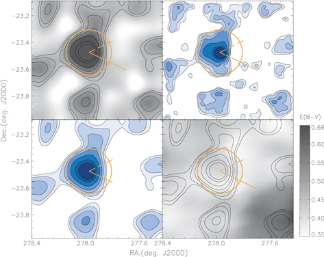
Figure 8. From top left to bottom right, the star count map around NGC 6642, the surface density maps smoothed by different Gaussian kernel values, and the E(B-V) extinction map around the cluster. The Gaussian kernel values are 0045 and 012. Isodensity contour levels are  and
and  . The circle indicates a tidal radius of NGC 6642. The solid line indicates the direction of the Galactic center and the dashed line shows the perpendicular direction of the Galactic plane.
Download figure:
Standard image High-resolution imageAs can be seen in Figure 8, the stellar distribution of NGC 6642 seems to show a drop in density around the tidal radius in the specific direction and clumpy structures outside of the tidal radius. However, the prominent extended stellar substructure elongates in a northern direction beyond the tidal radius. A clumpy chunk in the southern region seems to be a counterpart to the overdensity feature in the northern region. A marginal extension also appears in the eastern direction, which seems to be aligned with the opposite perpendicular direction to the Galactic plane. Unfortunately, we could not find substructures that might be associated with the proper motion of the cluster because the proper motion of NGC 6642 has not yet been reported.
The upper panel of Figure 9 shows the radial surface density profile of NGC 6642 along with the King model, the Wilson model, and the surface brightness profile of Trager et al. (1995). The radial surface profile of NGC 6642 shows an apparent overdensity feature that departs from both model predictions from a radius of log( ) ∼ 0.5
  to the tidal radius. However, the overdensity feature does not continue, and the density of the radial profile decreases abruptly at the tidal radius. The drop in density and local clumpy substructures around/outside the tidal radius shown in Figure 8 seem to be associated with this fall of the radial profile and low density feature at the outer region. The overdensity feature within the tidal radius was fitted by a power law with a slope
  .
.

Figure 9. Upper: radial surface density profile of NGC 6642 with the King model (solid curve) and the Wilson model (dotted line). There is an overdensity feature at  , which is represented by a power law, i.e., a dotted straight line in logarithmic scale with a slope of
  . The mean number density of stars in the overdensity region is estimated as
  per square arcmin. Lower: radial surface density profiles of eight different angular Sections (S1–S8). The radial density points, which were calculated by interpolation from neighboring densities, are indicated by the open triangle. The other notations are the same as those of the radial surface density profile in the upper panel.
Download figure:
Standard image High-resolution imageThe radial surface density profiles for eight angular sections, which are plotted in the lower panel of Figure 9, represent the stellar density distribution around NGC 6642 better than the average radial density profile in the upper panel of Figure 9. The radial profiles in the angular Sections 1 and 8 show clear overdensity features within a tidal radius, and Section 1 has the largest mean density of the eight sections. Although some radial points in these sections are not plotted because of small number statistics, there are still considerable number densities at the outer region. This is in agreement with the overdensity feature extending toward the eastern side on the two-dimensional surface density map. In contrast to these angular sections, the overdensity feature in Section 2 is disconnected at the tidal radius because of its low density at the outer region. In the two-dimensional surface contour map, we cannot find obvious stellar substructures in that region. The radial density profile in Section 3 shows the most prominent overdensity features with high density and the flattest slope, and contains a density excess at the outer radius. These are representative of a prominent extending substructure in the northern region on the isodensity contour map in Figure 8. In Section 7, the radial density profile is likely to show the overdensity feature associated with the counterpart of the extended substructure in the northern region. In Sections 4 and 5, we could not find a clear overdensity feature, and the two-dimensional contour map does not also show prominent stellar substructures in those regions.
4.4. NGC 6723
Figure 10 shows a star count map around NGC 6723, surface density maps smoothed with Gaussian kernel values of 007 and 011, and a distribution map of the E(B-V) value (Schlegel et al. 1998) from the upper left panel to the lower right panel. We note that different Gaussian kernel values for NGC 6723 were selected in order to highlight structures with similar spatial extents. Isodensity contours were overlaid on the maps with contour levels of  , and
, and  . The long dashed line and solid line indicate the direction perpendicular to the Galactic plane and the direction of the Galactic center, respectively. The proper motion of NGC 6723, i.e.,
  and
and  (Dinescu et al. 2003), is indicated with an arrow. The tidal radius of
  (Harris 1996) is represented by a circle.

Figure 10. From the top left to the bottom right panels, the star count map around NGC 6723, the surface density maps smoothed by Gaussian kernel values of 007 and 011, and the distribution map of E(B-V). Isodensity contour levels are  and
and  . The circle indicates the tidal radius of NGC 6723, the arrow represents the proper motion of the cluster, the solid line indicates the direction of the Galactic center, and the dashed line shows the perpendicular direction of the Galactic plane. We note that the direction to the Galactic center and the Galactic plane almost coincide, thus the two lines overlap each other.
Download figure:
Standard image High-resolution imageAs can be seen in Figure 10, there are weak extended substructures beyond the tidal radius of NGC 6723 at levels larger than σ. Small density lobes are likely to extend toward the eastern and western sides, toward the direction of the Galactic center, the direction perpendicular to the Galactic plane, or their opposite directions. In addition, the isodensity contour lines show a horn-shaped structure in the northern region, which corresponds to the direction opposite of the proper motion. The marginal extension appears near the tidal radius in the southern region, but this weak substructure does not seem to be growing outward anymore. We note that there is a huge reflection nebula in the distant souther region of the cluster. Thus, dust in the outskirts of the reflection nebula in the southern region could affect the detected number density of the marginal extension in the southern region. Indeed, the value of E(B-V) in the southeast region is higher than the values in other regions. Thus, there is a possibility that more extended stellar substructures could exist in the obscured region.
The radial surface densities for NGC 6723, measured in each concentric annulus, are shown in the upper panel of Figure 11. The theoretical King model and the Wilson model were arbitrarily normalized to our measurements, and the surface brightness profile of Trager et al. (1995) was used as a substitute for our measurements in the central region. Apparently, the radial number density profile departs from the theoretical King model at the outer region of the cluster, while the Wilson model has a slightly better fit to our radial profile of the cluster. The overdensity feature, which departs from the King model with a break in slope, is shown at a radius of log( ) ∼ 0.8 ( ∼ 0.6rt), and extends to a radius of log(
 ) ∼ 1.15 (∼1.5rt). The slope in this overdensity region is characterized by a power law with a slope of
  , which is steeper than the value predicted from a theoretical simulation with a constant orbit-averaged mass-loss rate (Johnston et al. 1999).

Figure 11. Upper: radial surface density profile of NGC 6723 with the King model (solid line) and the Wilson model (dotted line). The overdensity feature appears at the region of  . The overdensity feature is represented by a power law, i.e., a dotted straight line in logarithmic scale with a slope of
  . The mean number density of stars in the overdensity region is estimated as
  per square arcmin. Lower: radial surface density profiles of eight different angular Sections (S1–S8). For clarity, we magnified the radial profile of the overdensity feature. The other notations are the same as those of the radial surface density profile in the upper panel.
Download figure:
Standard image High-resolution image
The radial surface profiles of eight angular sections are also shown in the lower panel of Figure 11. The overdensity feature in the region of  is commonly detected in specific angular sections. The radial profile in Section 1, where the prominent substructure appears in the two-dimensional contour map, has the highest mean number density out of all the profiles of the eight sections. In addition, the densities in Sections 2, 5, and 8 have somewhat higher density levels in the overdensity region, which is in good agreement with the horn-shaped substructure, the side lobe in the west side, and the marginal structure in the south region shown in Figure 10. Some radial points near the tidal radius in Section 7 were not plotted because of the low number density. This low density feature also appears as a bay-shaped structure with low-level contours in the southern region on the contour map with a kernel value of 007. A possible narrow dust lane, which might extend from the reflection nebular in southern region, could be the cause of this low number density feature. Unfortunately, the extinction map of Schlegel et al. (1998) does not show an apparent dust lane because of its low resolution. Thus, a study of dust extinction with high resolution is necessary in order to study the stellar distribution around the cluster.
5. DISCUSSION
All of our target clusters reside within ∼3 kpc of the Galactic center. The ancient globular clusters in the inner region can provide clues regarding the formation of the Galactic bulge and disk. Indeed, the spatial, chemical, and kinematical properties of several globular clusters in the inner regions are consistent with those of bulge, disk, and even bar membership (Burkert & Smith 1997; Barbuy et al. 1998; Côté 1999; Heitsch & Richtler 1999). However, the definite decomposition of globular clusters between the bulge and disk or bar components is not a trivial task in the central region of the Galaxy because the inner regions of the Galaxy are superimposed by the various stellar populations from the bulge, the disk, and the bar. In addition, in the inner region of the Galaxy, globular clusters experience extreme dynamical evolution due to bulge/disk shock and strong tidal effects (Aguilar et al. 1988; Shin et al. 2008). Thus, reliable measurements of metallicities, orbits, and distances for globular clusters in the central regions are necessary in order to understand the evolution of the globular cluster in the bulge region. In this section, we investigated the previous results of our target globular clusters, and discussed the properties of clusters that could affect the substructures around globular clusters.
NGC 6266 is a high-density (log ; Jacoby et al. 2002; Possenti et al. 2003) and the ninth most luminous globular cluster located ∼1.7 kpc from the Galactic center (Harris 1996). Dinescu et al. (2003) found that NGC 6266 has a large rotation velocity, suggesting that this cluster belongs to a disk system rather than to a pressure-supported system. The total destruction rate of this cluster is about
  per Hubble time, and the destruction rate ratio is
  (Gnedin & Ostriker 1997), where
  is the evaporation rate per Hubble time. These destruction rates and ratios indicate that the main process of dynamical evolution for this cluster is internally driven, such as two-body relaxation. In this study, we found that apparent marginal extensions around the cluster bent toward the direction of proper motion and were likely to show S-shaped features. Thus, we can interpret this orientation of stellar substructure as the signature that the stars evaporated via internal two-body relaxation are finding themselves in a Galactic orbit similar to that of the parent cluster. However, we also found that the stellar density configuration around NGC 6266 shows a spatial coherence associated with the effect of dynamical interaction with the Galaxy. The prominent density feature extended toward the direction of the Galactic center. Thus, our stellar density distribution around NGC 6266 could be interpreted as an example of dynamical cluster evolution that tidal shocking accelerates two-body relaxation (Kundic & Ostriker 1995; Dinescu et al. 1999). Lee et al. (2007) classified NGC 6266 as an extended horizontal branch (EHB) cluster and also suggested that the clusters with EHB could be a remnant of the first building blocks in the early universe. Thus, the stellar density feature around NGC 6266 would be tidally associated with these unknown first building blocks. More accurate orbit information and an investigation of the field star contamination around NGC 6266 are necessary to understand the dynamical evolution of NGC 6266.
NGC 6626 is a massive and moderately metal-poor globular cluster in the Galactic bulge region. Dinescu et al. (1999) first found the thick-disk orbit for this cluster and then proposed the possibility that this cluster had been produced in a satellite galaxy and then departed from its parent during the accretion process. In addition, according to Lee et al. (2007), this cluster is a moderate EHB cluster and could be a remnant of the first building blocks. Chun et al. (2012) first found the stellar density substructure around NGC 6626, which extends toward the direction perpendicular to the Galactic plane, indicating a disk-shock effect. They also discussed the possibility of an accretion scenario for the origin of this cluster. More recently, Casetti-Dinescu et al. (2013) updated the proper motion and orbit of this cluster. They noted that the cluster is located at the apocenter and that its orbit is rather eccentric and disruptive, indicating that the cluster may experience substantial mass loss. In our study, we did find prominent stellar substructures extending toward the Galactic center and anti-center directions. This spatial orientation of the tidal tails is in good agreement with the findings of Montuori et al. (2007), namely, that the inner tails are oriented toward the direction of the Galactic center in the apocenter position. Moreover, we confirmed the stellar substructure extending toward the direction perpendicular to the Galactic plane, which was found by Chun et al. (2012). Casetti-Dinescu et al. (2013) mentioned that their newly updated proper motion vector with solar motion subtracted is aligned with this substructure. They then speculated that the recent disk plane crossing about 4 Myr ago might have contributed to the construction of a tidal extension in the direction perpendicular to the Galactic plane. Therefore, this cluster is very likely to suffer from disk/bulge shocks and Galactic tidal forces. However, the total destruction rate of  per Hubble time and the destruction ratio of
  by Gnedin & Ostriker (1997) do not seem to be in agreement with our interpretation. Thus, we note here that recalculation of the destruction rate is necessary using the recently updated proper motion and eccentric orbit.
NGC 6642 has dense central core with a high concentration c = 1.99 (Harris 1996). Previous studies (Trager et al. 1995; Balbinot et al. 2009) have also indicated that there is not a well-resolved core in the radial profile and have classified the cluster as a core-collapsed cluster. Barbuy et al. (2006) noted that the age of NGC 6642 is comparable to that of M5 and then suggested that the cluster is one of the few genuine metal-poor and old clusters in the bulge region. Therefore, it could contain fossil information about the Galaxy. On the other hand, Balbinot et al. (2009) examined the position of NGC 6642 in the HB type versus metallicity diagram and found that NGC 6642 lies at the position of young halo populations, not at the position of old halo and disk/bulge populations. They concluded that NGC 6626 is a transition cluster between the inner halo and outer bulge, considering its age, its position in the Galaxy, and its HB morphology. They also found clear evidence for the mass segregation and depletion of low-luminosity stars in the luminosity and mass function and attributed this dynamical structure to the disk and bulge shocking. Indeed, we did find clumpy stellar substructures that extend toward the north direction and the perpendicular direction opposite to the Galactic plane beyond the tidal radius. The large total destruction rate of  per Hubble time and the destruction ratio of
  by Gnedin & Ostriker (1997) also indicate that a strong environmental force, such as a tidal effect due to disk and bulge shocking, might affect the dynamical evolution of this cluster. Thus, we interpret that although NGC 6642 is a core-collapse cluster and two-body relaxation would affect the dynamical evolution of the cluster, the extended stellar substructures around NGC 6642 would be the result of a strong gravitational interaction with the Galaxy. Unfortunately, we were unable to investigate a definite association between the observed stellar substructure and the clusterʼs motion because there is no published proper motion information for this cluster. If we could obtain accurate proper motion for this cluster, we would be able to understand the dynamical evolution of the cluster and figure out the origin of the cluster, e.g., whether this cluster is a genuine metal-poor and old cluster in the bulge region or a transition cluster between the inner halo region and the outer bulge region.
NGC 6723, which has a relatively low concentration of density (c = 1.05, Harris 1996) and a moderate EHB morphology (Lee et al. 2007), is an old globular cluster in the Galactic bulge region. Although it has long been considered one of the genuine Galactic bulge globular clusters, the origin of the cluster is not obvious because there have only been a few studies of this cluster. van den Bergh (1993) suggested that NGC 6723 would have a circular orbit motion in the central region of the Galaxy. However, Dinescu et al. (2003) measured the proper motion of the cluster and found that its orbit is highly inclined. Based on its kinematics and low metallicity, they concluded that NGC 6723 is a member of the halo system. Recently, Lee et al. (2007) suggested a different origin scenario wherein metal-poor EHB globular clusters such as NGC 6723 would be relics of the first building blocks. The total destruction rate of  per Hubble time and a rather high destruction ratio of
  by Gnedin & Ostriker (1997) indicate that there would be weak tidal substructures around this cluster. Indeed, in our study, we have found tidal stripping features that are likely to be associated with the interaction with the Galaxy. The weak stellar density lobes, which extend toward the directions of the Galactic center and anti-center, were detected in the surface iso-density map. In addition, a marginal extension tracing the direction opposite to the proper motion was also detected. However, we could not exclude a dust extinction effect on the stellar density distribution map. The thin dust lane of a reflection nebula in the southern region of the cluster might hide stellar extensions.
6. SUMMARY
In this study, we investigated the stellar spatial density distribution around four metal-poor globular clusters (NGC 6266, NGC 6626, NGC 6642, and NGC 6723) in the Galactic bulge region using wide-field ( ) near-infrared
  and K images obtained with the WFCAM camera on UKIRT. In order to discard the field star contamination and enhance the density contrast between cluster member and field stars, we used the C–M mask filtering technique and the optimal contrast filtering technique on the cluster CMDs. Two-dimensional density contour maps of the clusters were examined, and radial density profiles were also investigated with the King and Wilson models.
The two-dimensional stellar density contour maps for the four globular clusters showed asymmetric and extended features of the stars around the globular clusters. In particularly, three globular clusters (NGC 6266, NGC 6626, and NGC 6642) showed tidal extension and a stellar chunk beyond the tidal radius while NGC 6723 showed weak density lobes near the tidal radius. Such extended stellar substructures were aligned with the direction of the Galactic center and anti-center, the direction perpendicular to the Galactic plane, or the direction of the cluster orbit motion. Thus, it is highly probable that target clusters are affected by the dynamical environment effect such as a tidal force and bulge/disk shock. The radial profile also represented the extended substructures in the two-dimensional contour maps as overdensity features with a break in a slope. Although the observed radial profiles of clusters departed from the King and Wilson models at the outer region of the cluster, the Wilson model appeared to have a better fit with the observed radial density profile for the cluster, which seemed to experience less of a dynamical environment effect (e.g., NGC 6266 and NGC 6723).
We note here that internal drivers such as two-body relaxations, also affect the extended stellar substructure around the globular clusters. The stellar extensions around NGC 6266 show a good example of internal drivers. In this cluster, the stars might have primarily evaporated due to a two-body relaxation, and then could have been affected by the environmental tidal force of the Galaxy. For other clusters, it is obvious that the two-body relaxation contributes to the extended stellar substructures around clusters. In contrast to the case of NGC 6266, however, environmental effects such as the tidal force of the Galaxy and bulge/disk shock would be main factors for the extended stellar substructures, even though clusters such as NGC 6642 had very active two-body relaxations. In addition, a more accurate proper motion and orbit that are calculated using an accurate galaxy potential model could increase the portion of the external effect on the dynamical evolution of the globular clusters in the bulge region. Indeed, although the tidal-shock rate of NGC 6626 was not comparable to or larger than the two-body relaxation rates in previous studies (Gnedin & Ostriker 1997; Dinescu et al. 1999), the orbit of NGC 6626, which was derived using more accurate proper motion and an axisymmetric and barred model of the Galaxy (Casetti-Dinescu et al. 2013), was found to be eccentric and more disruptive. Therefore, further studies of the dynamical evolution of the globular clusters in the bulge region with accurate proper motion and a galaxy model are required to provide theoretical constraints of the configuration of stars around globular clusters. In addition, further deep and wide-field photometric data for metal-poor and metal-rich globular clusters in the Galactic bulge could provide more accurate information about the dynamical evolution of globular clusters, thereby leading to an increased understanding of the origin of globular clusters in the bulge region as well as the formation of the bulge region.
We are grateful to an anonymous referee for detailed comments that greatly improved this paper. This research was supported by the Basic Science Research Program through the National Research Foundation of Korea (NRF) funded by the Ministry of Education, Science, and Technology (2013R1A1A2006826). The authors are grateful for partial support from the KASI–Yonsei DRC program of the Korea Research Council of Fundamental Science and Technology (DRC-12-2-KASI).