

Abstract
We review the evidence for a putative early 21st-century divergence between global mean surface temperature (GMST) and Coupled Model Intercomparison Project Phase 5 (CMIP5) projections. We provide a systematic comparison between temperatures and projections using historical versions of GMST products and historical versions of model projections that existed at the times when claims about a divergence were made. The comparisons are conducted with a variety of statistical techniques that correct for problems in previous work, including using continuous trends and a Monte Carlo approach to simulate internal variability. The results show that there is no robust statistical evidence for a divergence between models and observations. The impression of a divergence early in the 21st century was caused by various biases in model interpretation and in the observations, and was unsupported by robust statistics.
Export citation and abstract BibTeX RIS

Original content from this work may be used under the terms of the Creative Commons Attribution 3.0 licence. Any further distribution of this work must maintain attribution to the author(s) and the title of the work, journal citation and DOI.
1. Introduction
A presumed slowdown in global warming during the first decade of the 21st century, and an alleged divergence between projections from climate models and observations, have attracted considerable research attention. Even though the Earth's climate has long been known to fluctuate on a range of temporal scales (Climate Research Committee, National Research Council 1995), the most recent fluctuation has been singled out as a seemingly unique phenomenon, being identified as 'the pause' or 'the hiatus.' By the end of 2017, the 'pause' had been the subject of more than 200 peer-reviewed articles (Risbey et al 2018).
Here, we focus on one aspect of the putative 'pause'; namely, an alleged divergence between model projections and observed global mean surface temperature (GMST); in particular the claim that climate models over-estimated warming (Fyfe et al 2013). The question of whether GMST deviates from model projections has often been conflated with, but is conceptually distinct from, questions relating to the observed warming rate. For example, one might ask whether warming has ceased or 'paused' or entered a 'hiatus'. Answers to this question involve tests of the statistical hypothesis that the warming trend is equal to zero. A different question might be whether warming has slowed significantly, in which case the statistical question is whether there is a change in the long-term rate of warming. A third question, at issue in this article, is whether the observations diverge from model-derived expectations.
Existing research on the 'pause' has often conflated the distinct questions that can be asked about short-term warming trends. This conflation can be problematic because it is possible, in principle, for the observations to diverge from model-derived expectations even though warming continues unabated. Under those circumstances it would be misleading to discuss a 'pause' or 'slowdown', notwithstanding any divergence between projected and observed trends.
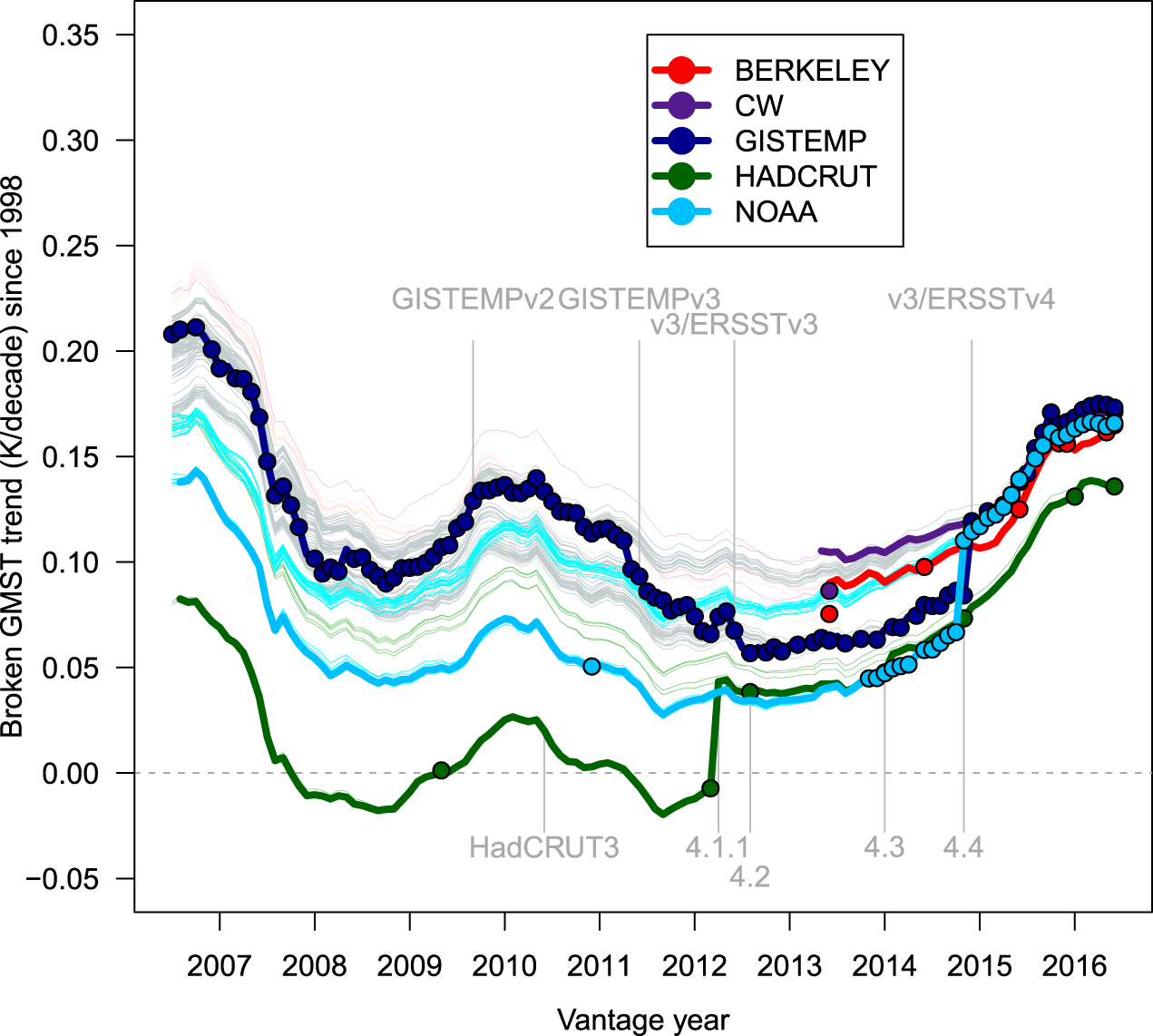
A further difficulty in interpreting research on the 'pause' is that this period of intense research activity coincided with notable improvements to observational datasets. Specifically, GMST datasets are evolving over time as they extend coverage (Morice et al 2012), introduce or modify interpolation methods that fill-in data for areas in which observations are sparse (Cowtan and Way 2014), or remove biases arising from issues such as the transition of sea surface temperature (SST) measurement from ships to buoys (Karl et al 2015, Hausfather et al 2017). In consequence, research on short-term warming trends may come to different conclusions, depending on what version of a dataset is being used. Figure 1, adapted from the companion article by Risbey et al (2018), shows that the consequences of revisions to GMST datasets are far from trivial. The figure shows GMST trends starting in 1998 and ending at the times marked on the x-axis (vantage points). Each solid line shows what we call 'historically-conditioned' trends, which reflect only data that were available at each vantage point. The thin lines, by contrast, show the retrospective ('hindsight') trends calculated back to earlier vantage points as if the later versions of the dataset had been available then.
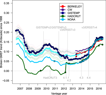
Figure 1. Historically conditioned trends for major GMST datasets; Berkeley (Cowtan and Way 2014); the U.K. Met Office's HadCRUT (Brohan et al 2006, Morice et al 2012); NASA's GISTEMP (Hansen et al 2010); Cowtan and Way's improved version of HadCRUT (Cowtan and Way 2014); and NOAA's dataset (Vose et al 2012). Each solid line plots the best-fitting least squares trend from the start year of 1998 to the end year (vantage year) as shown on the x-axis. The thick lines for each dataset correspond to the version available and current at a given vantage year, with the vertical gray lines indicating major changes in version. The thin lines provide retrospective trends that show what the trends would have been if later versions of the data (represented by solid points) had been available earlier. The solid points indicate the dates of versions of each dataset that were available for analysis. The trends are incremented from monthly data which results in some fine scale variation.
Download figure:
Standard image High-resolution imageThe figure shows that different versions of the same dataset can yield substantially different trend estimates, as indicated by the difference between each solid line and its thinner retrospective counterparts. This is particularly pronounced for HadCRUT, which shows a distinct jump in 2012 when HadCRUT3 was replaced by HadCRUT4. In consequence, a data analyst using HadCRUT3 in early 2012 would have concluded that the warming trend since 1998 had been slightly negative, whereas the same analyst using HadCRUT4 some months later would have concluded that warming since 1998 had been positive. Likewise, although the datasets are known to yield similar long-term estimates of global warming (e.g. from 1970 to the present), there were considerable differences between datasets for short-term trends early in the 21st century. See Risbey et al (2018) for details.
In this article, we apply the same historical conditioning to our analysis of the putative divergence between models and observations during the period known as the 'pause.' That is, we use the variants of the datasets that were available at the time when assessing evidence for the divergence between models and observations, and we also condition the model projections on the estimates of the forcings on the climate system that were available at any given time. The historical conditioning of both models and observations provides the most like-with-like assessment of the divergence between models and observations.
In order to assess claims made about this putative divergence we searched the literature for articles (published through 2016) that referred to a 'pause' or 'hiatus' in GMST in the title or abstract. The search was completed in December 2017 and yielded 225 peer-reviewed articles (see Risbey et al 2018 for a complete list). On the basis of the abstracts, 82 of those articles were identified as being concerned with a potential divergence between the model projections and observations during the 'pause' period. (An additional 6 articles mentioned the putative divergence but did not examine it.) From this initial set of 82, we extracted a corpus of articles (N = 50) that explicitly defined a start and end date for the period of interest, and that also specified the GMST dataset used for analysis. This is the minimum amount of information required to reproduce and examine the claims about a divergence between models and observations made in those articles. Table 1 provides the citations for those articles together with information about the period examined and the observational dataset used.
Table 1. Articles in the corpus with start and end date of presumed 'pause' and observational datasets being considered (G = GISTEMP, H3 = HadCRUT3, H4 = HadCRUT4).
| Years | Observational dataset | |||||
|---|---|---|---|---|---|---|
| Citation | Start | End | G | H3 | H4 | Other |
| Allan et al (2014) | 2000 | 2012 | * | ERA-Interim | ||
| Brown et al (2015) | 2002 | 2013 | * | |||
| Chikamoto et al (2016) | 2000 | 2013 | * | ERSST 4 | ||
| Dai et al (2015) | 2000 | 2013 | * | * | ||
| Delworth et al (2015) | 2002 | 2013 | * | |||
| Easterling and Wehner (2009) | 1998 | 2008 | ||||
| England et al (2014) | 2001 | 2013 | * | |||
| England et al (2015) | 2000 | 2013 | Cowtan and Way | |||
| Fyfe et al (2013) | 1998 | 2012 | * | |||
| Fyfe et al (2016) | 2001 | 2014 | * | * | RSS, UAH | |
| Gettelman et al (2015) | 1998 | 2014 | * | * | * | |
| Gu et al (2016) | 1999 | 2014 | * | ERSST | ||
| Haywood et al (2014) | 2003 | 2012 | * | |||
| Huber and Knutti (2014) | 1998 | 2012 | * | Cowtan and Way | ||
| Hunt (2011) | 1999 | 2009 | * | |||
| Kay et al (2015) | 1995 | 2015 | * | * | ||
| Knutson et al (2016) | 1998 | 2016 | * | * | ||
| Kosaka and Xie (2013) | 2001 | 2013 | * | |||
| Kosaka and Xie (2016) | 1998 | 2016 | * | * | ||
| Kumar et al (2016) | 1999 | 2013 | * | * | ||
| Li and Baker (2016) | 1998 | 2012 | * | |||
| Lin and Huybers (2016) | 1998 | 2014 | * | |||
| Lovejoy (2014) | 1998 | 2013 | * | |||
| Lovejoy (2015) | 1998 | 2015 | * | |||
| Mann et al (2016) | 2001 | 2011 | * | Kaplan SST, HadISST, ERSST | ||
| Marotzke and Forster (2015) | 1998 | 2012 | * | |||
| Meehl and Teng (2012) | 2001 | 2010 | * | NCEP/NCAR | ||
| Meehl et al (2014) | 2000 | 2013 | * | |||
| Meehl et al (2016) | 2001 | 2016 | * | * | HadISST | |
| Meehl et al (2016) | 2000 | 2013 | NCEP/NCAR | |||
| Pasini et al (2017) | 2001 | 2014 | * | |||
| Peyser et al (2016) | 1998 | 2012 | * | * | ||
| Power et al (2017) | 1997 | 2014 | * | |||
| Pretis et al (2015) | 2001 | 2013 | * | |||
| Rackow et al (2018) | 1998 | 2012 | * | HadISST, ERA-Interim | ||
| Risbey et al (2014) | 1998 | 2012 | * | * | Cowtan and Way | |
| Roberts et al (2015) | 2000 | 2014 | * | * | HadSST | |
| Saenko et al (2016) | 2003 | 2013 | * | |||
| Saffioti et al (2015) | 1998 | 2012 | * | ERA-Interim, JRA-55, NCEP/NCAR, NCEP/DOE, NOAA 20CR | ||
| Schmidt et al (2014) | 1997 | 2013 | * | Cowtan and Way | ||
| Schurer et al (2015) | 1998 | 2013 | * | |||
| Smith et al (2016) | 2001 | 2016 | * | * | ||
| Steinman et al (2015b) | 2004 | 2013 | * | HadISST, ERSST, Kaplan SST | ||
| Thoma et al (2015) | 1998 | 2015 | * | ERA40 | ||
| Thorne et al (2015) | 1998 | 2012 | * | * | BERKELEY, Cowtan and Way | |
| Wang et al (2017) | 2001 | 2015 | * | * | ||
| Watanabe et al (2013) | 2001 | 2013 | * | * | ||
| Watanabe et al (2014) | 2001 | 2012 | * | JRA-55, HadiSST1 | ||
| Wei and Qiao (2016) | 1998 | 2014 | * | |||
| Zeng and Geil (2016) | 1998 | 2012 | * | * | BERKELEY | |
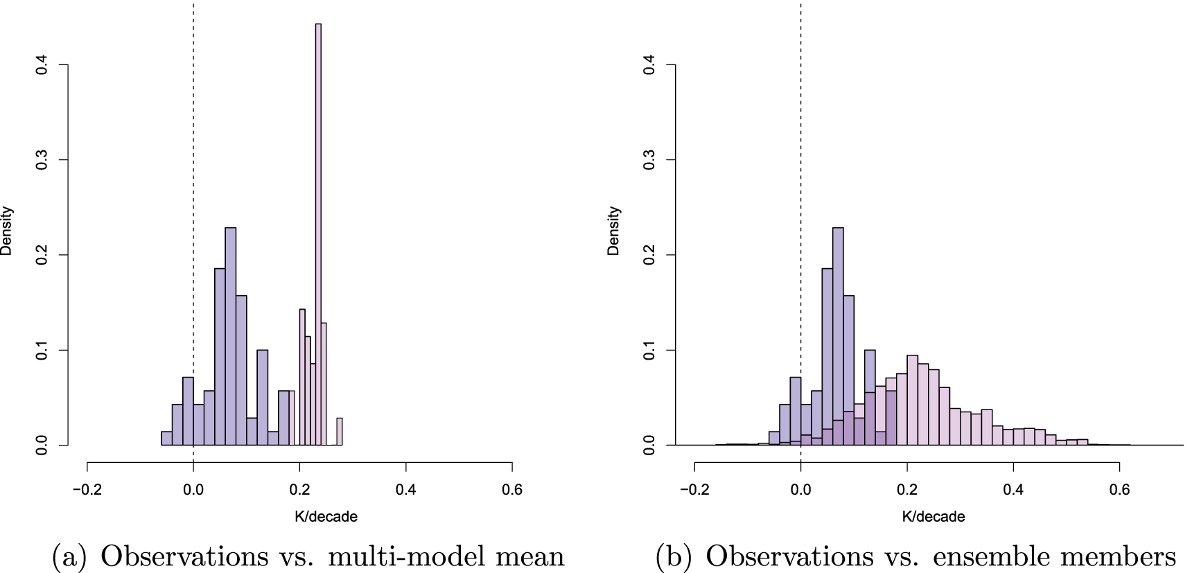
We summarize this literature graphically. Figure 2 shows the observed and modeled warming rates for the time periods covered in the corpus. For each article, we compute a warming trend using the dataset and period specified in the article. The average duration of trends being examined was 14.6 years (median = 15, range 10–21). The same period is used to obtain a trend for comparison from the CMIP5 simulations.
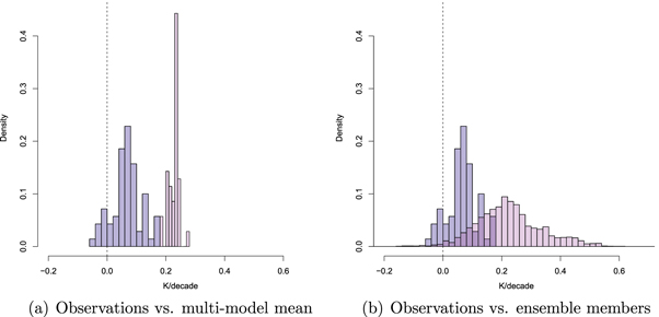
Figure 2. Normalized density distribution of observed decadal temperature trends (blue) and the corresponding trends in the CMIP5 simulations (pink). For the observations, the dataset and time periods were as in the corpus of published articles (N = 50) on the apparent divergence between models and observations. An article contributes multiple observations if multiple datasets were used. The same time periods were used to construct the modeled distribution of trends from globally averaged surface air temperatures (TAS). Model runs are as in table 3 and used the original forcings from the CMIP5 experiments. Historical runs are spliced together with RCP8.5. Panel (a) shows the trends for the multi-model mean only, and panel (b) shows the trends for all CMIP5 ensemble members.
Download figure:
Standard image High-resolution imageConsider first panel (a) in the figure. The blue histogram shows the observations and the pink histogram shows the modeled trends using the CMIP5 multi-model mean. All trends are computed based on the information provided in the articles in the corpus, and each article contributes at least one observation (or more, if an article used multiple datasets). It is clear that the articles in the corpus were mainly concerned with time periods in which GMST was either increasing only slightly or even decreased. At first glance, panel (a) also gives the appearance that observed warming trends lagged behind model-derived expectations for the time periods considered in the corpus. Accordingly, some articles in the corpus draw strong conclusions about a divergence between models and observations, stating for example that 'Recent observed global warming is significantly less than that simulated by climate models' (Fyfe et al 2013, p 767), or 'global-mean surface temperature (T) has shown no discernible warming since about 2000, in sharp contrast to model simulations, which on average project strong warming' (Dai et al 2015, p 555). These conclusions were reflected in the most recent IPCC Assessment Report (AR5), which examined the match between observed GMST and the CMIP5 historical realizations (extended by the RCP4.5 forcing scenario for the period 2006–2012). The IPCC stated that '...111 out of 114 realizations show a GMST trend over 1998–2012 that is higher than the entire HadCRUT4 trend ensemble ... . This difference between simulated and observed trends could be caused by some combination of (a) internal climate variability, (b) missing or incorrect radiative forcing and (c) model response error' (Flato et al 2013, p 769). The consensus view expressed by the IPCC therefore pointed to a divergence between modeled and observed temperature trends, putatively caused by a mix of three factors. Subsequent to the IPCC report, the role of these three factors has become clearer.
The contribution of internal climate variability to the putative divergence between models and observations has been illustrated in several ways. First, when internal variability is considered by selecting only those models whose internal variability happens to be aligned with the observed phase of the El Niño Southern Oscillation (ENSO; Trenberth 2001), which is a major determinant of tropical Pacific SSTs, the divergence between observed and modeled GMST trends during the 'pause' period is reduced considerably or even eliminated (Meehl et al 2014, Risbey et al 2014). Second, when only those (few) model realizations are considered that—by chance alignment of their modeled internal variability to that actually observed—reproduced the observed 'pause', their warming projections for the end of the century do not differ from those of the remaining realizations that diverged from observations during the recent period (England et al 2015). These findings show that any conclusions about a divergence between observed and modeled trends that are based on the CMIP5 multi-model mean are highly problematic. The multi-model mean does not capture the internal variability of the climate system—on the contrary, the mean cancels out that internal variability, and observed GMST therefore cannot be expected to track the mean but rather should behave like a single model realization. The observed climate is, after all, a single realization of a stochastic system.
The importance of internal variability is illustrated in panel (b) in figure 2, which shows the same observed trends from our corpus against a distribution of modeled trends for all CMIP5 ensemble members. Unlike the multi-model mean in panel (a), the distribution of trends modeled by the different ensemble members is far broader and spans the observed trends because different ensemble members are in different states of internal variability at any given simulated time. Consideration of internal variability thus reduces the alleged divergence between modeled and observed trends.
Concerning radiative forcings, the possible inadequacies anticipated by the IPCC (Flato et al 2013) have been confirmed by subsequent research (Huber and Knutti 2014, Schmidt et al 2014). We explore the implications of updated forcings in detail below.
Concerning model response error, it is notable that the IPCC report did not consider potential biases in the observations as an alternative variable, even though the differences between datasets were known at the time (figure 1). The analysis presented here shows that when biases in observations and model output are considered and corrected, then there is no discernible divergence between models and observations. There is no evidence of model response error, or that the models are 'running too hot.' Our analysis also shows that statistical evidence for a divergence between models and observations was apparent only for a brief period (2011–2013), before those biases were addressed. Even then, that interpretation was marred by questionable statistical choices.
2. Methods and data
2.1. Overview
We ask whether there is any divergence between GMST trends, as captured by the major observational datasets, and the Coupled Model Intercomparison Project Phase 5 (CMIP5) projections during the last 20–25 years. The principal analyses are historically conditioned for both observations and model projections. That is, analysis at any given temporal vantage point involves the observational data and projections that were available at that point in time.
We differentiate between different ways in which short-term trends can be computed relative to the long-term trend, and we take into account the statistical ramifications of selecting a trend because it is low before conducting a statistical test. This problem is known as 'selection bias' or the 'multiple-testing problem'.
Our main analysis relies on a Monte Carlo approach to generate a synthetic distribution of internal climate variability. This distribution provides a statistical reference distribution against which the observed GMST trends can be compared to assess their probability of occurrence on the basis of internal variability alone.
All data used in the analyses and the R scripts can be accessed at https://git.io/fAur5.
2.2. Observational datasets
We use four observational datasets that are summarized in table 2. To economize presentation, we omitted the NOAA dataset (Vose et al 2012). All of these datasets have undergone revisions to debias their estimates of GMST. For details, see Risbey et al (2018). Our analysis used versions of the GMST datasets as they existed at different points in time over the 'pause' research period.
Table 2. GMST datasets used in the analysis (with labels used in figure captions). The release dates specify when the data was made publicly available. If no release date is given, the dataset had been in use before research on the 'pause' commenced. If coverage of a dataset is global, then it is compared to global output of the CMIP5 model projections. If parts of the globe are not covered (HadCRUT), then the model output is masked to the same coverage for comparison.
| Dataset (label in captions) | Released | SST data | Model output | Citation |
|---|---|---|---|---|
| Berkeley (BERKELEY) | March 2014 | HadSST3 | Global | Rohde et al (2013) |
| Cowtan and Way (CW) | November 2013 | HadSST3 | Global | Cowtan and Way (2014) |
| GISTEMP (GISTEMP) | HadSST2 + OISST pre 2013 | Global | Hansen et al (2010) | |
| ERSSTv3 til mid 2015 | ||||
| ERSSTv4 after mid 2015 | ||||
| HadCRUT3 (HADCRUT) | HadSST2 | Masked | Brohan et al (2006) | |
| HadCRUT4 (HADCRUT) | November 2012 | HadSST3 | Masked | Morice et al (2012) |
All analyses reported here have been performed with all four of the datasets shown in table 2. To economize presentation, we usually focus on GISTEMP and HadCRUT because they were available throughout the period of research into the 'pause' and hence permit accurate historical conditioning. GISTEMP and HadCRUT also bracket the magnitude of the warming trends observed during the 'pause' (see figure 1), with HadCRUT providing the lowest estimates (in part because it omits a significant number of grid cells in the high Arctic, which is known to warm particularly rapidly), and GISTEMP providing a higher estimate of warming throughout (because it provides coverage of the Arctic by interpolation).
All of the datasets were limited to the period 1880–2016, with anomalies computed relative to a common reference period of 1981–2010. This reference period was chosen because the different SST records are most consistent over this period, and it avoids the recent changes in ship bias (Kent et al 2017). All trends were computed using ordinary least squares. The auto-correlation structure of the data is, however, modeled in the main Monte Carlo analysis.
2.3. Model projections
An ensemble of 84 CMIP5 historical multimodel runs was combined with RCP8.5 projections to yield simulated and projected GMST for the period 1880–2016. RCP8.5 makes the most extreme assumptions about increases in forcings and therefore provides the 'hottest' scenario for comparison to the GMST data, rendering it most suitable for the detection of any divergence between rapid projections and slow actual warming. Table 3 lists the models used and their runs.
Table 3. CMIP5 models and number of original runs used in the analysis. Each historical run is concatenated with the corresponding RCP8.5 projection. All model output is baselined with reference to the period 1981–2010. The multi-model mean was computed by averaging across all runs for each model first, before averaging across models.
| Model name | N model runsa |
|---|---|
| ACCESS1 | 2 |
| bcc-csm1 | 1 |
| CanESM2 | 5 |
| CCSM4 | 6 |
| CESM1-BGC | 1 |
| CESM1-CAM5 | 3 |
| CMCC-CM | 1 |
| CNRM-CM5 | 6 |
| CSIRO-Mk3-6-0 | 10 |
| EC-EARTH | 5 |
| FIO-ESM | 3 |
| GFDL-CM3 | 1 |
| GFDL-ESM2G | 1 |
| GFDL-ESM2M | 1 |
| GISS-E2-H-CC | 1 |
| GISS-E2-H | 5 |
| GISS-E2-R-CC | 1 |
| GISS-E2-R | 5 |
| HadGEM2-AO | 1 |
| HadGEM2-CC | 1 |
| HadGEM2-ES | 4 |
| inmcm4 | 1 |
| IPSL-CM5A-LR | 4 |
| IPSL-CM5A-MR | 1 |
| IPSL-CM5B-LR | 1 |
| MIROC-ESM-CHEM | 1 |
| MIROC-ESM | 1 |
| MIROC5 | 3 |
| MPI-ESM-LR | 3 |
| MPI-ESM-MR | 1 |
| MRI-CGCM3 | 1 |
| MRI-ESM1 | 1 |
| NorESM1-M | 1 |
| NorESM1-ME | 1 |
aFor some models, the physical properties differed between runs. We averaged across all runs irrespective of physics.
Where applicable, model output was masked to the coverage of the corresponding dataset (HadCRUT; see table 2). The masked model results were treated in the same way as the corresponding data; namely, by averaging separate hemispheric means to obtain GMST. This approach mirrors HadCRUT (both versions 3 and 4), which also uses hemispheric averages to produce a global mean, rather than averaging all grid cells across both hemispheres simultaneously (Brohan et al 2006, Morice et al 2012). We therefore report comparisons involving HadCRUT separately from comparisons involving the other datasets.
The CMIP5 model projections have undergone two notable revisions since 2013.
2.3.1. Updated forcings
Climate projections are obtained by applying estimates of the historical radiative forcings for historical runs (until 2005), followed by the future forcings that are assumed by the scenario (e.g. RCP8.5). If those presumed forcings turn out to be wrong, for example because economic activity or climate policies follow an unexpected path or because historical estimates are revised, then any divergence between modeled and observed GMST cannot be used to question the suitability or accuracy of climate models (Flato et al 2013).
Relevant variables such as volcanic eruptions, aerosols in the atmosphere, and solar activity all took unexpected turns early in the 21st century, necessitating an update to the original presumed forcings in the RCPs which had created a warm bias in the model projections. Two such updates have been provided (Huber and Knutti 2014, Schmidt et al 2014).
The updated estimates provided by Schmidt et al (2014) became available early in 2014 (27 February) and covered the period 1989–2013. Schmidt et al (2014) identified four necessary adjustments to (a) well-mixed greenhouse gases (WMGHG; correcting a small cool bias in the projections); (b) solar irradiance (correcting a warm bias from around 1998 onward); (c) anthropogenic tropospheric aerosols (correcting a warm bias from around 1998 onward); and (d) volcanic stratospheric aerosols (correcting a substantial cool bias around 1992 and a growing warm bias since 1998). The adjusted forcings were converted into updated GMST using an impulse-response model (Boucher and Reddy 2008).
The alternative updated forcings provided by Huber and Knutti (2014) became available later in 2014 (17 August) and covered the period 1970–2012. Huber and Knutti (2014) did not update the forcings from WMGHGs or anthropogenic tropospheric aerosols, focusing instead on solar irradiation and statospheric aerosols only. Huber and Knutti (2014) used two separate estimates to correct for solar irradiation, by the Active Cavity Radiometer Irradiance Monitor and by the Physikalisch-Meterologisches Observatorium Davos (PMOD). Huber and Knutti (2014) also provided two updated estimates of stratospheric aerosols. One estimate, roughly paralleling that used by Schmidt et al (2014), relied on optical thickness estimates from NASA GISS. The other estimate additionally considered 'background' stratospheric aerosols unconnected to volcanic eruptions (Solomon et al 2011). Huber and Knutti (2014) used a climate model of intermediate complexity (Stocker et al 1992) to estimate the effect of the updated forcings on GMST.
In our analyses we report model projections with two sets of adjustments: First, the total adjustments provided by Schmidt et al (2014), referred to as S-adjusted from here on. Second, we report the adjustments provided by Huber and Knutti (2014) using the PMOD estimates of solar irradiation and without consideration of background aerosols (H-adjusted from here on). Those adjustments replace the assumed zero-forcings for 2001–2005 for volcanic aerosols in the historical RCPs (Meinshausen et al 2011). The H-adjusted projections almost certainly under-estimate the warm bias in the RCP forcings and thus provide a lower bound of the possible effects of updated forcings.
For both sets we carried forward the final adjustments to subsequent years. We also made the simplifying assumption that both adjustments were available from the beginning of 2014 onward to facilitate annualizing of the updated projections.
2.3.2. Blending of air and SST
The second revision of model projections involved the recognition that the models' global near-surface air temperature (coded as TAS in the CMIP5 output), which had commonly been compared with observational estimates of GMST, was not strictly commensurate with the observations (Cowtan et al 2015). (See also Santer et al 2000, Knutson et al 2013 and Marotzke and Forster 2015) GMST is obtained by combining air temperature measurements from land-based stations with SSTs measured in the top few meters of the ocean. A true like-with-like comparison of models to observations would therefore involve a similar blend of modeled land temperatures and modeled SST (coded as TOS).
Cowtan et al (2015) showed that if the HadCRUT4 blending algorithm is replicated on the CMIP5 model outputs, the divergence between model projections and observations is reduced by about a quarter (during 2009–2013). The insight that like-with-like comparison required blending of model output became available half-way through 201510 .
For our analyses, we blended land-air (TAS) and sea-surface (TOS) anomalies from the models for comparison to the observations, with air temperature used over sea ice. For comparison to HadCRUT3 or HadCRUT4, the blended anomalies are masked to observational coverage before calculation of hemispheric means, whereas for the remaining observational records the global mean of the spatially complete blended field is used.
2.4. Historical and hindsight trends
As already noted in connection with figure 1, when the latest available GMST datasets are used (defined here as through the end of 2016), we term this a 'hindsight' analysis because the current GMST data benefit from all bias reductions made to date, irrespective of what time period is being plotted or analyzed. To accurately represent the information available to researchers at any earlier point in time, we focus on a historically-conditioned analysis that uses the versions of each of the datasets that were current at the time in question.
We provide the same historical conditioning for the CMIP5 model projections based on the two major revisions just discussed. Because the revisions to the forcings involve two alternative adjustments (S-adjusted versus H-adjusted), we use both in our historically-conditioned analysis. In addition, when models are compared to the HadCRUT datasets, historical conditioning entails a change in the coverage mask between HadCRUT3 and HadCRUT4 to mirror the change in coverage between the two datasets.
2.5. Continuous and broken trends
The trends shown in figure 1 were computed following the common approach in the literature, by computing a trend between a start and end date by estimating a slope and intercept for the regression line. Computation of the trend in this manner introduces a break between contiguous trend lines if the period before (or after) the trend in question is modeled by a separate linear regression (Rahmstorf et al 2017). This is problematic for several reasons: first, for short-term trends, an independent estimate of slope and intercept becomes particularly sensitive to the choice of start and end points. Second, any break at the junction of two contiguous trends calls for a physical explanation. Although temperature trends are often modeled based on statistical considerations alone, the statistical models cannot help but describe a physical process—any break in the long-term trend line therefore tacitly invokes the presence of a physical process that is responsible for this break and intercept shift. No such process has been proposed or explicitly modeled. Third, even ignoring the absence of an underlying physical process, a broken trend cannot be interpreted as just a 'slowdown' in warming: a correct interpretation must include the shift in intercept, for example by stating that 'after a jump in temperatures warming was less than before the jump.' The interpretations of broken trends in the literature generally fail to mention the intercept shift.
The solution to this problem is to compute short-term trends that are continuous: when partial trends are continuous, they converge at a common point and share that 'hinge', even though the slopes of the two partial trends may differ (Rahmstorf et al 2017). In comparing short-term GMST trends against the modeled trends we show results for both broken and continuous trends.
2.6. Selection bias
Most of the articles written on the 'pause' fail to offer any justification for the choice of start year. Published start years span the range from 1995 to 2004, with the modal year being 1998 (Risbey et al 2018). This broad range may be indicative of a lack of formal or scientific procedures to establish the onset of the 'pause.' Moreover, in each instance the presumed onset of the 'pause' was not randomly chosen, but specifically because of the subsequent low trend (Lewandowsky et al 2015). However, therein lies a problem: if a period is chosen (from many possible such time intervals) because of its unusually low trend, this has implications for the interpretation of conventional significance levels (i.e. p-values) of the trend (Rahmstorf et al 2017). Selection of observations based on the same data that is then being statistically tested inflates the actual p-value, thereby giving rise to a larger proportion of statistical Type I errors than the researcher is led to expect (Wagenmakers 2007). Very few articles on the 'pause' account for or even mention this effect, yet it has profound implications for the interpretation of the statistical results. Rahmstorf et al (2017) referred to this issue as the 'multiple testing problem,' although here we prefer the term 'selection bias' because we find it to be more readily accessible. More appropriate techniques exist (Rahmstorf et al 2017) and are used in our statistical testing.
2.7. Statistical testing
Because GMST is not expected to track the multi-model mean, any divergence between models and observations must be evaluated with respect to how unusual it is in light of the expected internal variability of the climate system. We generate those expectations by decomposition of the observed warming into a forced component and internal variability. Observed trends can then be evaluated against the expectations derived from that internal-variability component.
The forced component is a composite of anthropogenic influences such as warming from greenhouse gases and cooling from tropospheric aerosols, and natural components such as volcanic activity and solar irradiation. Internal variability is superimposed on this time-varying forced signal. Observed GMST (T) can thus be expressed as:

where Fa and Fn represent anthropogenic and natural forcings, respectively, and Vp–n represents pure internal variability. The term E is a composite term that refers to all sources of error and bias, such as structural uncertainty in models and observations (Cowtan et al 2018) and uncertainties in the observations (Morice et al 2012).
We estimate:


where Vn represents the single actual historical realization of the internal variability component of the Earth's climate, including errors and biases that escape quantification but that we implicitly model during our analysis. The CMIP5 multi-model ensemble mean is taken to represent the total forced signal, Fa + Fn (Dai et al 2015, Knight 2009, Mann et al 2014, 2016, 2017, Steinman et al 2015a, 2015b). To equalize the weight given to each model irrespective of how many runs it contributes to the ensemble (table 3), we average runs within each model before averaging across models.
We use all data from the period 1880–2016 to compute the residual (Vn) by subtracting the CMIP5 multi-model ensemble mean from the observations. We use this single observed realization to estimate the stationary stochastic time series model that best describes internal variability (and its unknown error component). Specifically, we model Vn computed by equation (3) with a selection of ARMA(p, q) models, where p ∈ {0, 1, 2, 3} and q ∈ {0, 1, 2, 3} and choose the most appropriate model on the basis of minimum AIC. This model is then used to generate, via Monte Carlo simulations, a synthetic ensemble of realizations (N = 1000) of internal variability that conform to the statistical attributes revealed by the chosen ARMA model. These realizations provide a synthetic reference distribution of residuals for comparison against the observations. To make this comparison commensurate with the reference distribution, the observations are represented by the trend of the residuals between GMST and the CMIP5 multi-model mean. Thus, when reporting the results (figures 9 through 12), all trends refer to the trend in the residuals during the period of interest. This comparison takes into account autocorrelations in the GMST data as the synthetic realizations capture the observed autocorrelational structure of the GMST time series11 .
We report the result of that comparison as the percentage of synthetic trends with a magnitude smaller than the trend of interest. For a trend to be considered unusual—and hence divergent from model-derived expectations—fewer than 5% of all synthetic trends must be lower than the observed trend of interest.
3. Results
3.1. Comparing models to observations
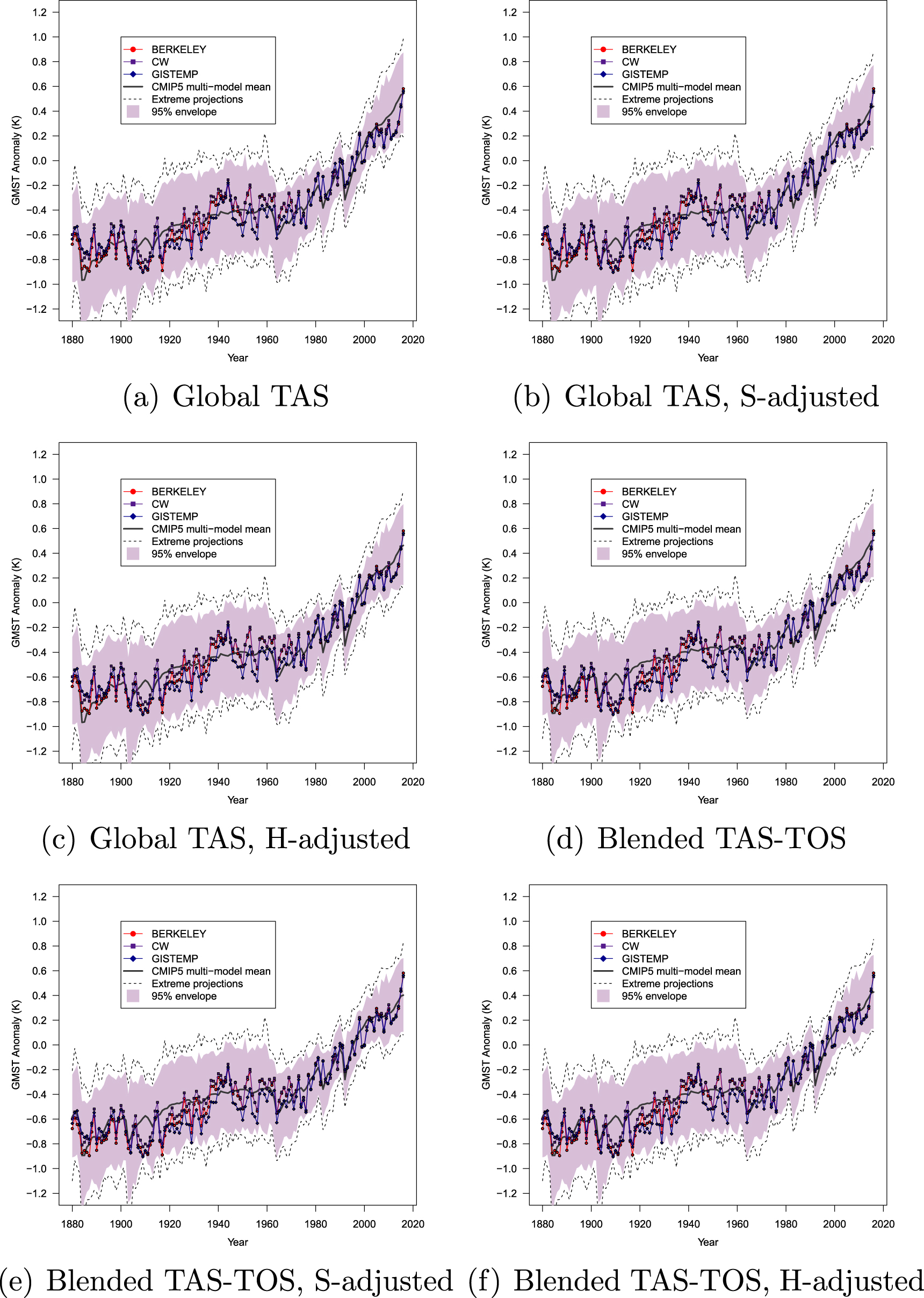
Figures 3 and 4 show the latest available GMST data against the model projections. Figure 3 shows the GMST datasets with global coverage and figure 4 shows the HadCRUT4 dataset with limited coverage (and correspondingly masked model output).

Figure 3. Hindsight comparison of latest available global GMST datasets with CMIP5 model projections. The solid black line represents the multi-ensemble mean and dotted lines the most extreme model runs. The shaded area encloses 95% of model projections. Both GMST and model projections are anomalies relative to a reference period 1981–2010. The top-left panel (a) presents the conventional comparison using global air surface (TAS) from the models. Panels (b) and (c) also use global TAS but with forcings adjusted as per Schmidt et al (2014) or Huber and Knutti (2014), respectively. Panel (d) uses blend of TAS and sea surface temperature (TOS) in models. Panels (e) and (f) also use blended temperatures but with forcings adjusted as per Schmidt et al (2014) or Huber and Knutti (2014), respectively.
Download figure:
Standard image High-resolution image
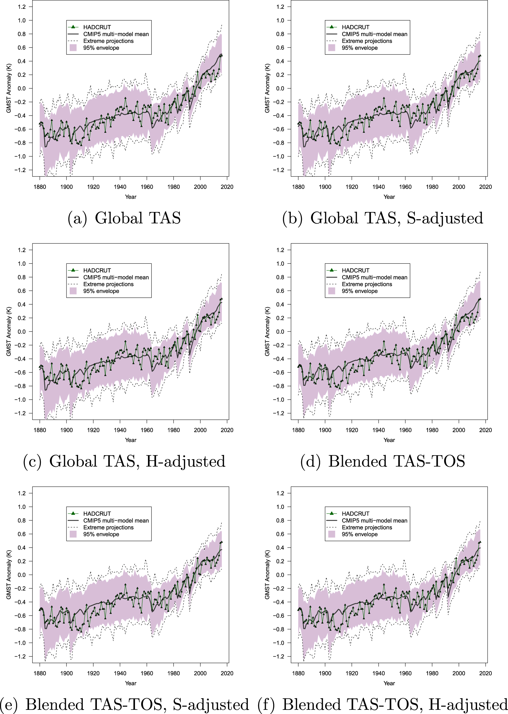
Figure 4. Hindsight comparison of latest available HadCRUT4 dataset with CMIP5 model projections masked to the same coverage as the observations. The solid black line represents the multi-ensemble mean and dotted lines the most extreme model runs. The shaded area encloses 95% of model projections. Both GMST and model projections are anomalies relative to a reference period from 1981 to 2010. The top-left panel (a) presents the conventional comparison using global air surface (TAS) from the models. Panels (b) and (c) also use global TAS but with forcings adjusted as per Schmidt et al (2014) or Huber and Knutti (2014), respectively. Panel (d) uses blend of TAS and sea surface temperature (TOS) in models. Panels (e) and (f) also use blended temperatures but with forcings adjusted as per Schmidt et al (2014) or Huber and Knutti (2014), respectively.
Download figure:
Standard image High-resolution imageIn each figure, the different panels show the effects of historical conditioning of the model projections. The top-left panels (a) show the conventional comparison between CMIP5 global air surface temperatures (TAS) and GMST that constituted the most readily available means of comparison until 2015. Panels (d) show a more appropriate, like-with-like comparison between the GMST data and the models, with both model output and observations being blended between land-air (TAS) and sea-surface (TOS) temperatures in an identical manner. This comparison became available in 2015 (Cowtan et al 2015).
Comparison of panels (a) and (d) clarifies that blending of the model output reduces the divergence between models and observations early in the 21st century. The apparent divergence was exaggerated by the long-standing but nonetheless inappropriate use of TAS as the sole basis for comparison. Panels (b), (c), (e) and (f) in the figures additionally show the effects of adjusting the forcings. The adjustments were applied to global TAS output (panels (b) and (c) for S-adjusted and H-adjusted, respectively) as well as blended TAS-TOS output (panels (e) and (f) for S-adjusted and H-adjusted, respectively).
It is clear from these results that when the updated forcings are applied and model output is blended between TAS and TOS in the same way as the observations (panels (e) and (f)), there is no discernible divergence between model projections and GMST. It matters little whether the comprehensive S-adjustments or the overly conservative H-adjustments are applied to the model projections. Notably, the only apparent recent divergence arises with the HadCRUT dataset without adjustment of the forcings (panels (a) and (d) in figure 4).
We explore the results presented in figures 3 and 4 with detailed trend analyses.
3.2. Broken and continuous trends
We first examine the impact of how short-term trends are computed, by comparing broken to continuous trends.
Considering first the broken trends, figures 5 and 6 plot observed and modeled 15 year trends. The figures contrast hindsight (top panels) to historically-conditioned perspectives (bottom panels) on the model projections and observations. The historically-conditioned panels therefore omit datasets that only became available recently (BERKELEY and CW). Figure 5 shows the datasets with global coverage and global model projections, whereas figure 6 shows the HadCRUT dataset with model output masked to the same coverage.
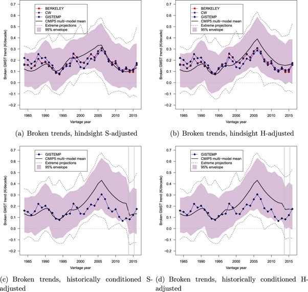
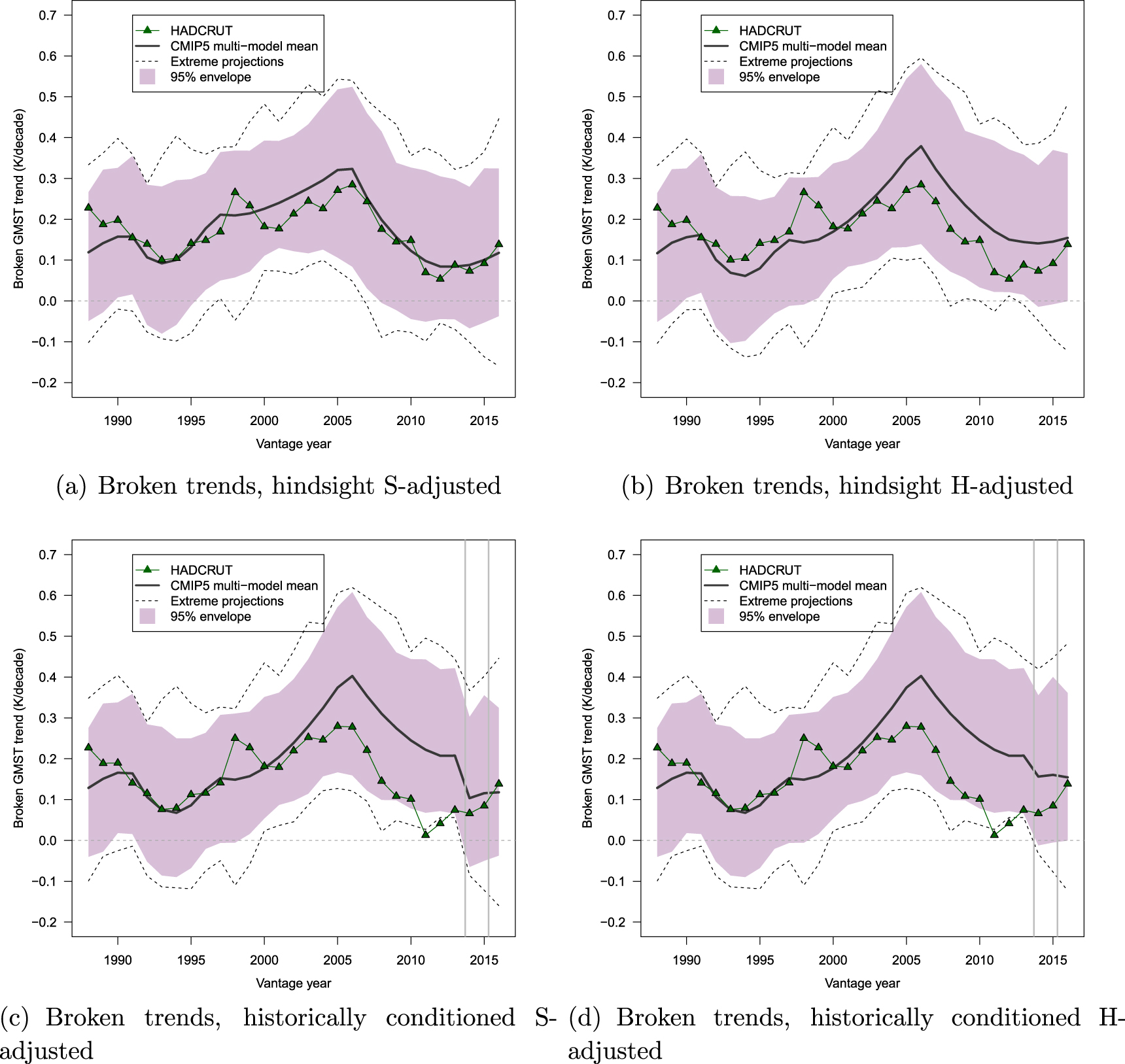
Figure 5. Comparison of 15 year broken trends between model projections and observations. Each trend is plotted with the end year as vantage year and is shown in K/decade. The solid black line represents the multi-ensemble model mean and dashed lines the most extreme model runs. The shaded area encloses 95% of model projections. Panels (a) and (b) provide a hindsight perspective, using the latest available datasets with global coverage and TAS-TOS blended model output with updated forcings. Panel (a) uses corrections to forcings provided by Schmidt et al (2014) and panel (b) uses corrections provided by Huber and Knutti (2014). Panels (c) and (d) provide a historically-conditioned perspective on data and models, and therefore omit datasets not available throughout. Vertical lines indicate major revisions to CMIP5 model output or interpretation (forcings adjustment and blending). Panel (c) uses corrections to forcings provided by Schmidt et al (2014) from 2014 onward and panel (d) uses corrections provided by Huber and Knutti (2014) also from 2014 onward.
Download figure:
Standard image High-resolution image
Figure 6. Comparison of 15 year broken trends between model projections and observations. Each trend is plotted with the end year as vantage year and is shown in K/decade. The solid black line represents the multi-ensemble model mean and dashed lines the most extreme model runs. The shaded area encloses 95% of model projections. Panels (a) and (b) provide a hindsight perspective, using the latest available version of HadCRUT4 and TAS-TOS blended model output with updated forcings masked to the same coverage. Panel (a) uses corrections to forcings provided by Schmidt et al (2014) and panel (b) uses corrections provided by Huber and Knutti (2014). Panels (c) and (d) provide a historically-conditioned perspective on data and models. Vertical lines indicate major revisions to CMIP5 model output or interpretation (forcings adjustment and blending). Panel (c) uses corrections to forcings provided by Schmidt et al (2014) from 2014 onward and Panel (d) uses corrections provided by Huber and Knutti (2014) also from 2014 onward. Note that transition from HadCRUT3 to HadCRUT4 is accompanied by a change in the model mask as coverage between the two versions differs.
Download figure:
Standard image High-resolution imageEach trend is computed for the 15 year period ending in the vantage year being plotted. Each panel only includes data after the onset of modern global warming, as determined by a change-point analysis for each dataset (Cahill et al 2015). Thus, the earliest vantage year in each figure is 15 years after the onset of modern global warming in that dataset. In each figure, panels (a) and (b) provide a hindsight view of the model projections and observations, using the updated forcings and TAS-TOS blending throughout. Panels (c) and (d), by contrast, provide a historically-conditioned perspective on the model projections and observations, with the vertical lines indicating the time when revisions to forcings and blending of TAS and TOS became available. Panels (c) use S-adjustments and panels (d) use H-adjustments, respectively.
It is clear from figures 5 and 6 that in hindsight there is no evidence for a divergence between models and observations. The pattern differs for the historically-conditioned analyses, which show some divergence between observations and models early in the 21st century. This divergence is particularly apparent with HadCRUT (figure 6), for the years immediately preceding the switch from HadCRUT3 to HadCRUT4.
Turning to continuous trends, figures 7 and 8 support broadly similar conclusions. In hindsight, there is little evidence for any divergence between models and observations. With historical conditioning, a divergence was observable early in the 21st century and this divergence was particularly pronounced for HadCRUT3.

Figure 7. Comparison of 15 year continuous trends between model projections and observations. Each trend is plotted with the end year as vantage year and is shown in K/decade. The solid black line represents the multi-ensemble model mean and dashed lines the most extreme model runs. The shaded area encloses 95% of model projections. Panels (a) and (b) provide a hindsight perspective, using the latest available datasets with global coverage and TAS-TOS blended model output with updated forcings. Panel (a) uses corrections to forcings provided by Schmidt et al (2014) and panel (b) uses corrections provided by Huber and Knutti (2014). Panels (c) and (d) provide a historically-conditioned perspective on data and models, and therefore omit datasets not available throughout. Vertical lines indicate major revisions to CMIP5 model output or interpretation (forcings adjustment and blending). Panel (c) uses corrections to forcings provided by Schmidt et al (2014) from 2014 onward and panel (d) uses corrections provided by Huber and Knutti (2014) also from 2014 onward.
Download figure:
Standard image High-resolution image
Figure 8. Comparison of 15 year continuous trends between model projections and observations. Each trend is plotted with the end year as vantage year and is shown in K/decade. The solid black line represents the multi-ensemble model mean and dashed lines the most extreme model runs. The shaded area encloses 95% of model projections. Panels (a) and (b) provide a hindsight perspective, using the latest available version of HadCRUT4 and TAS-TOS blended model output with updated forcings masked to the same coverage. Panel (a) uses corrections to forcings provided by Schmidt et al (2014) and panel (b) uses corrections provided by Huber and Knutti (2014). Panels (c) and (d) provide a historically-conditioned perspective on data and models. Vertical lines indicate major revisions to CMIP5 model output or interpretation (forcings adjustment and blending). Panel (c) uses corrections to forcings provided by Schmidt et al (2014) from 2014 onward and panel (d) uses corrections provided by Huber and Knutti (2014) also from 2014 onward. Note that transition from HadCRUT3 to HadCRUT4 is accompanied by a change in the model mask as coverage between the two versions differs.
Download figure:
Standard image High-resolution image3.3. Statistical comparison
Our principal statistical analysis follows up on the data just reported (figures 5 through 8) using the Monte Carlo approach outlined earlier. We ask whether at any time during the decade from 2007 to 2016 there was statistical evidence for a divergence between the observed GMST trend since 1998 (the modal start year of the 'pause' identified in the literature; Risbey et al 2018) and the model projections. Only historically-conditioned observations and model projections are considered, although for the final year in question (2016) the conditioned data are identical to the hindsight perspective. Because of the historical focus, datasets that were not available until recently are not considered (BERKELEY and CW).
Figures 9 and 10 summarize the statistical analyses using broken trends for GISTEMP and HadCRUT, respectively. In each figure, the top row of panels show statistical comparisons involving the 'pause' period only, whereas those at the bottom involve comparisons of the presumed 'pause' period to the entire record of internal variability represented in the reference distribution of synthetic realizations. The bottom panels therefore deal with the selection-bias problem explained in section 2.6 whereas the top panels do not correct for this bias, as is common in the literature.
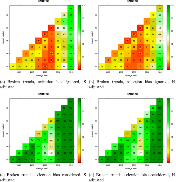
Figure 9. Monte Carlo comparison of broken GMST trends (GISTEMP) to a reference distribution of synthetic realizations of internal variability. Cell entries refer to the percentage of synthetic trends lower than that observed. See text for how trends are computed. Values below 5% are circled in yellow to indicate statistical significance. Vantage years refer to the end point of the trends being examined and both models and observations are historically-conditioned for that time.
Download figure:
Standard image High-resolution image
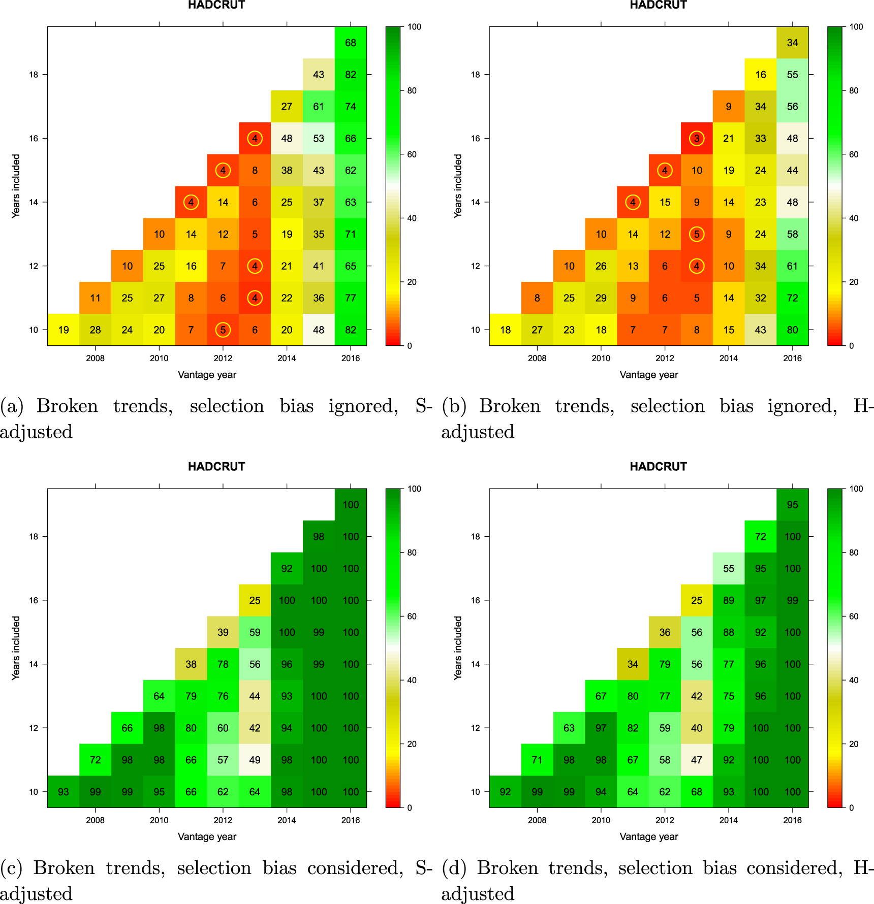
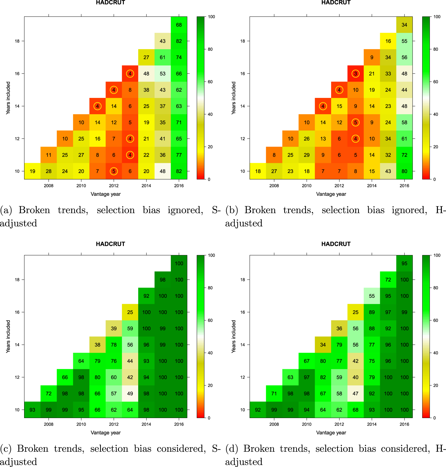
Figure 10. Monte Carlo comparison of broken GMST trends (HadCRUT) to a reference distribution of synthetic realizations of internal variability. Cell entries refer to the percentage of synthetic trends lower than that observed. See text for how trends are computed. Values below 5% are circled in yellow to indicate statistical significance. Vantage years refer to the end point of the trends being examined and both models and observations are historically-conditioned for that time.
Download figure:
Standard image High-resolution imageWithin each panel, a matrix of potential 'pause' periods is represented. The vantage year (x-axis) is the last year of each potential pause-period during the last decade, and the number of years included (y-axis) defines how far back the pause-interval extends. Trends are extended only as far back as 1998 (all cells on the diagonal involve 1998 as the start year).
For every candidate 'pause' defined in the matrix, the divergence of the corresponding observed GMST trend from the CMIP5 multi-model mean was compared against the synthetic realizations of internal variability obtained by Monte Carlo (section 2.7). When comparison involved only the 'pause' period (top panels in the figures), the observed candidate 'pause' was compared against the synthetic ensemble for that particular duration and time period only. The percentage of synthetic trends lower than the observed trend is reported in the corresponding cell in the matrix. Values below 5% are additionally identified by a yellow circle as they are deemed to represent a significant divergence between modeled and observed temperatures beyond that expected on the basis of internal variability alone. If none of the synthetic trends are smaller than the observed trend, the percentage will be zero—indicating that models are warming significantly faster than the observations. The comparison is single-tailed, so cells can take on large values if the observed trend is sufficiently positive.
When the selection-bias problem was accounted for (bottom panels in the figures), the observed candidate 'pause' was compared against each possible trend of the same duration at all possible times in each synthetic realization since the onset of modern global warming. (The onset year was determined separately for each dataset based on the analysis reported by Cahill et al 2015.) The cell entries record the percentage of synthetic realizations in which at least one such trend fell below the observed candidate 'pause' trend. This percentage can be interpreted as 'how unusual is the observed trend in light of what would be expected to arise due to internal variability alone at some point in time during global warming'.
Interpretation of the results in figures 9 and 10 is straightforward. First, irrespective of which dataset is being considered or which adjustment to model projections is applied, when the selection-bias problem is accounted for, there has been no evidence at any time between 2007 and 2016 for the hypothesis that observations lagged significantly behind model-derived expectations (bottom panels of figures 9 and 10). This conclusion holds for any trend commencing in 1998 or later with a minimum duration of at least 10 years. (It is not meaningful to consider shorter trends. This is reflected in the literature on the 'pause' which consensually focuses on trends 10 years or longer; see figure 1 in Risbey et al 2018.)
Second, when the selection-bias problem is ignored (top panels of figures 9 and 10), there was apparent evidence of a statistically significant divergence between models and observations from around 2011–2013. That is, during those three years in history, researchers would have had access to statistical evidence for an apparent divergence.
Figures 11 and 12 provide another perspective on the same analysis using continuous trends. We noted in section 2.5 that many investigators had used broken trends in their analyses. However, as shown by Rahmstorf et al (2017), in the absence of independent evidence of a change in the forcing functions or other identifiable change in conditions of the system, inferring a change in the rate of warming on the basis of broken trends is unwarranted, and may produce misleading results. In this instance, the figures show that the conclusions are largely unchanged with continuous trends.
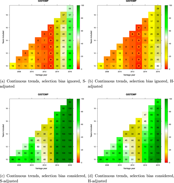
Figure 11. Monte Carlo comparison of continuous GMST trends (GISTEMP) to a reference distribution of synthetic realizations of internal variability. Cell entries refer to the percentage of synthetic trends lower than that observed. See text for how trends are computed. Values below 5% are circled in yellow to indicate statistical significance. Vantage years refer to the end point of the trends being examined and both models and observations are historically-conditioned for that time.
Download figure:
Standard image High-resolution image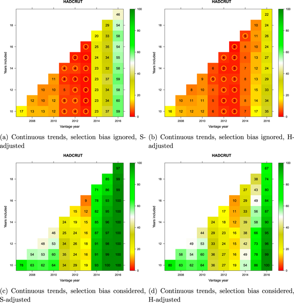
Figure 12. Monte Carlo comparison of continuous GMST trends (HadCRUT) to a reference distribution of synthetic realizations of internal variability. Cell entries refer to the percentage of synthetic trends lower than that observed. See text for how trends are computed. Values below 5% are circled in yellow to indicate statistical significance. Vantage years refer to the end point of the trends being examined and both models and observations are historically-conditioned for that time.
Download figure:
Standard image High-resolution image4. Implications
We asked whether there was a meaningful divergence between climate-model projections and GMST during the 21st century. We explored a multi-dimensional statistical and conceptual space that simultaneously considered (a) the historical evolution of GMST datasets, (b) historical revisions to the CMIP5 projections and their interpretation, (c) different ways of computing trends, and (d) different ways in which to test hypotheses about the divergence between models and observations. The results of our exploration converge on two conclusions.
First, there is no evidence, using currently available observations and model projections, for a significant divergence between models and observations during the last 20 years. This conclusion generalizes across datasets (GISTEMP and HadCRUT) and it does not depend on any other choices during data analysis.
Second, when models and observations are historically conditioned, the strength of apparent evidence for a divergence between models and observations crucially depends on the statistical comparison being employed. When the statistical tests take into account the fact that the period under consideration was chosen for examination based on its apparent low trend, thereby accounting for the selection-bias problem (section 2.6), no evidence for a divergence between models and observations existed at any time during the last decade. This conclusion holds irrespective of how trends are computed (broken versus continuous; section 2.5). When the selection-bias problem is ignored, by contrast, apparent evidence for a divergence between models and observations existed between 2011 and 2013 irrespective of which dataset (GISTEMP versus HadCRUT) is considered and how trends are computed (broken versus continuous).
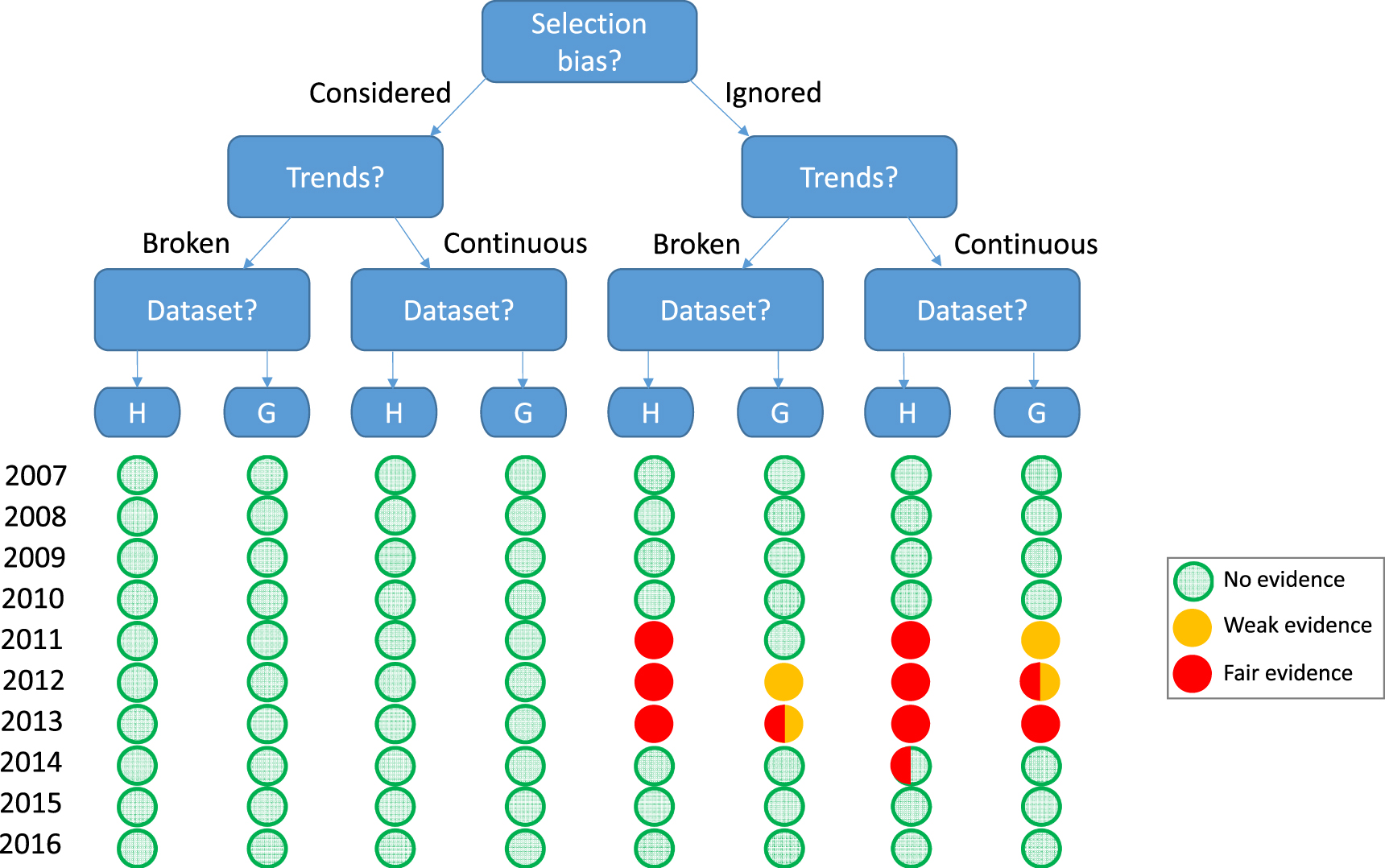
Figure 13 summarizes the Monte Carlo analysis in a decision tree that outlines the major options for analysis. The tree captures the fact that researchers must make several choices about the analysis. They must decide whether or not to correct for the selection-bias issue (the top decision node in the figure). They must decide how to model the pause-interval (as broken or continuous trends; second level of decision nodes). They must choose which dataset to use (HadCRUT or GISTEMP; third level). The tree pinpoints the conditions under which—and when—apparent evidence for a divergence existed. The state of the evidence is represented by the leaves of the tree (small circles) at the bottom of the figure. Green leaves denote absence of evidence, defined as more than half of all possible trend durations in that vantage year exceeding the bottom 10% of synthetic realizations. Any leaf that is partially or wholly orange or red signals the appearance of some degree of evidence for a divergence between observations and model projections. The evidence is considered poor (orange leaves) if half or more of all possible trend durations in that vantage year fall below the bottom 10% of synthetic realizations. The evidence is considered fair (red leaves) if, in addition, there is at least one trend in that vantage year falls below the bottom 5% of synthetic realizations. It is clear that any such evidence was limited to the time period 2011–2013 and only emerged when the selection-bias problem was ignored.
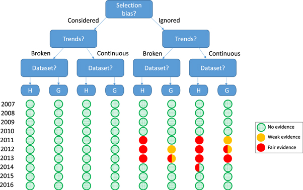
Figure 13. Tree representation of the results of the present analysis. The analysis either considers or ignores the selection-bias problem; the trends are estimated either as broken or continuous; and the GMST data can come from HadCRUT (H) or GISTEMP (G). The leaves (circles) at the bottom represent the results of a historically-conditioned analysis of all trends since 1998 at each year indicated (figures 9 through 12). Leaves are colored to reflect the level of apparent evidence for a divergence between models and observations, with green denoting the absence of evidence, orange denoting weak evidence and red denoting fair evidence (see text for explanation). Half circles denote the appearance of evidence with only one of the adjustments to forcings (S-adjustments versus H-adjustments).
Download figure:
Standard image High-resolution imageThe pattern in the figure is reflected in the corpus of 50 articles on the divergence between models and observations: 31 of those articles (62%) considered a period that ended in one of the three years (2011, 2012, and 2013) during which the evidence for a divergence from models appeared strongest. A further eight considered a period ending in 2014.
The delineation of the apparent evidence in figure 13 gives rise to two important questions: first, can the choices that give rise to the apparent divergence be justified? Second, why was the apparent evidence limited to the years 2011–2013, and would that evidence have been detectable if observations and models had already been debiased at that time?
4.1. Data analytic choices
The impression that observations diverged from model projections arose only when analysts ignored the selection bias issue. Figure 9 though 12 underscore the generality of these results: in all figures, the bottom panels (selection bias considered) showed no evidence for any divergence, whereas the top panels (selection bias ignored) give a different impression, with varying degrees of apparent divergence.
The problem that arises from the selection-bias issue—namely an inflation of the Type I error rate—was discussed and accounted for by Rahmstorf et al (2017), although they left the magnitude of the problem unspecified. We quantified the problem using a Monte Carlo approach derived from the analysis method just reported.
We generated a new set of 1000 synthetic realizations as described earlier. The CMIP5 multi-model mean was based on TAS/TOS blended global anomalies using S-adjusted forcings. The observations were from GISTEMP. The ensemble of 1000 realizations was then used in a Monte Carlo experiment involving 100 replications. On each replication, a single realization was sampled from the ensemble at random, which was taken to constitute the 'observations' for that replication. From that critical realization, a single 15 year trend (either broken or continuous) was chosen for statistical comparison with the remaining realizations in the ensemble. The trend was chosen in one of several ways: (a) A trend was picked at random by choosing any possible starting date between the onset of global warming (1970 for GISTEMP) and 2002 with equal probability. (b) The lowest 15 year trend observed since onset of global warming (1970) in the critical realization was selected. (c) The second-lowest trend was selected from the critical realization. (d) The trend at the 10th percentile of all possible trends was chosen.
Each chosen trend was then compared against 15 year trends with identical start and end dates across the remaining realizations in the ensemble. This comparison is exactly analogous to the variant of our main analysis that ignored the selection-bias issue.
Because all realizations, including the one chosen as the 'observations' for a given replication, share an identical random structure, the null hypothesis that temperatures are driven by internal variability alone is known to be true. A single randomly-chosen trend would therefore be expected to fall in the middle of that comparison distribution, with approximately half of all comparison trends falling above and below the chosen trend, respectively. Only occasionally should the randomly-chosen trend be in the extremes of the distribution. Specifically, by chance alone, only 5% of the time should the randomly-chosen trend fall below the 5th percentile of the comparison distribution (in which case the trend would be falsely identified as 'significantly lower than expected'). Likewise, no more than 10% of the time should the randomly-chosen trend fall below the 10th percentile of the comparison distribution and so on.
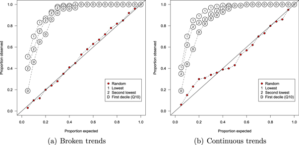
Figure 14 shows the results by plotting the proportion of times (out of 100 replications) that the comparison trend fell below the indicated percentile of the distribution of trends in the synthetic ensemble. Panel (a) shows the results for broken trend, and panel (b) for continuous trends.
Figure 14. Monte Carlo illustration of the consequences of ignoring the selection-bias issue. A 15 year trend is chosen from a random realization of internal variability (1970–2016) and is then compared to the remaining realizations in the ensemble at the same point in time. The trend can be chosen randomly, that is by randomly selecting a start year, or it can be the lowest or second-lowest in that realization, or it can be at the first decile (10th quantile) of all possible trends in that realization. A randomly chosen trend falls into the expected position in the distribution of comparison realizations (e.g. 5% of the time it sits below the 5th percentile and so on). Cherry-picked trends lead to inflated Type I errors. Panel (a): broken trends. Panel (b): continuous trends. See text for details.
Download figure:
Standard image High-resolution image
For both types of trend, the randomly-chosen trend closely tracks the diagonal, thereby mirroring the distribution expected under the null hypothesis. That is, in about half of the replications the trend was near the median of the ensemble realizations, in about a quarter of replications the trend fell around the first quartile of the ensemble, and so on. Assuming a significance threshold of 0.05, the observed Type I error rate for the randomly-chosen trend is thus around 5%, as expected.
A very different pattern is observed for trends that were chosen on the basis of their low magnitude in the critical realization. For example, when the lowest trend in the critical realization was chosen and then compared to the remaining synthetic realizations, in nearly half of the replications this trend was lower than the 5th percentile of the comparison distribution—put another way, the Type I error rate was vastly inflated beyond the nominal 5%. The problem is attenuated for trends that are less extreme (i.e. second-lowest trend or a trend at the 10th percentile of all possible trends in the critical realization), but in all cases and for both types of trend the magnitude-based selection inflates the Type I error rate, again as expected.
The figure illustrates the essence of the selection-bias problem: whenever a trend is chosen because its magnitude is particularly low, subsequent statistical tests that seemingly confirm the unusual nature of the trend yield an inflated number of false positives. In our corpus of articles, 79% of all reported 'pause' trends were below the first decile in the distribution of all possible trends of equal duration in the dataset, and 54% of reported trends were the lowest observed since the onset of global warming (mean percentile 0.073). It follows that around half of all 'pause' trends considered in the literature would have been classified as deviating significantly from model projections with a probability of around 50% even if GMST had evolved exactly as expected on the basis of the forcings with superimposed natural variability.
It follows that the common practice in the 'pause' literature to ignore the selection-bias issue inadvertently facilitated erroneous conclusions about the putative divergence between models and observations.
4.2. Debiasing of observations and models
The hindsight analysis (represented by the bottom row for 2016 in figure 13 and the rightmost columns in figures 9 though 12) differs considerably from the historical-conditioning results. This difference arises from two factors, namely the incremental reduction of a cool bias in the observations during the last 10 years (figure 1) and the parallel reduction of a warm bias in the CMIP5 model projections (e.g. figure 5, panels (c) and (d)).
We ask three questions about the debiasing: Would there have been any appearance of a divergence between models and observations if the debiasing had already been available in 2011–2013? How robust are the choices that were made during debiasing of observations and models? Were those biases known (or at least knowable) at the time when articles reported a divergence between models and observations?
4.2.1. Debiasing: the historical counterfactual
Figure 1 illustrated the effects of gradual debiasing on the observed GMST trends since 1998. The figure also contained counterfactual information, represented by the thin lines which indicate what the trend would have been at an earlier time, had the later debiasing been available then. We can apply the same counterfactual analysis to the debiasing of the models, namely by blending TAS/TOS throughout rather than just after its implications became widely known in 2015 (Cowtan et al 2015). Likewise, the adjustment to forcings that became available in 2014 (Huber and Knutti 2014, Schmidt et al 2014) can be applied to the model output before that time.
These counterfactual data were presented in the top panels (a) and (b) of the earlier figures 5 through 8. It is clear from those figures that had the debiasing been available earlier, no discernible divergence between models and observations would have been detected. By implication, it is unlikely that there would have been a literature on a putative 'pause' or an alleged divergence between models and observations if observations and model projections had been debiased a decade earlier.
Given the notable role of the debiasing, we must examine whether those adjustments to observations and models were robust and sufficiently justified.
4.2.2. Robust debiasing
Two major sources of bias have been identified and corrected in the observational datasets: these are data coverage (Rohde et al 2013, Cowtan and Way 2014), and the bias reduction of SST data (Karl et al 2015, Hausfather et al 2017). Both of those corrections have been shown to be necessary and robust.
There are multiple lines of independent evidence that confirm the bias that arises from limited data coverage, in particular in the HadCRUT dataset which omits a significant number of grid cells in the high Arctic, particularly over the Arctic ocean. The bias is shown in figure 1 as the difference between datasets with global coverage (e.g. GISTEMP, CW, BERKELEY) and the HadCRUT dataset. The CW dataset (Cowtan and Way 2014) is based on HadCRUT but extends coverage to the Arctic (and other regions omitted in HadCRUT) by interpolation. The robustness of that interpolation has been established by extensive cross-validation (Cowtan and Way 2014). The estimates provided in CW for the Arctic also agree with reanalyses, such as the ERA-interim reanalysis (Simmons and Poli 2015, Simmons et al 2017) and JRA-55 reanalysis (Simmons et al 2017). The BERKELEY dataset also achieves global coverage by interpolation but uses a different approach from CW and relies on data that are collected and analyzed independently from HadCRUT (Cowtan et al 2015). Notwithstanding, BERKELEY closely tracks CW in figure 1. The fact that multiple approaches to interpolation converge on the same bias correction supports their robustness.
Similarly, there are multiple lines of evidence that show earlier versions of SST to have suffered from a cool bias. The cool bias in recent SST records arises from the increasing prevalence of drifting buoy observations. The bias was first reported by Smith et al (2008), and was initially addressed by Kennedy et al (2011). Subsequent work has identified a further bias in the ship data, which when addressed further increases trends over the pause period (Huang et al 2015, Hausfather et al 2017).
Turning to biases in the model output, the conventional use of TAS (surface air temperatures) for comparisons with observations was less appropriate than the blending of TAS and TOS (modeled SST) (Cowtan et al 2015). Given that all observational datasets blend surface air temperature measurements over land with SST measurements, the blended data permit a more like-with-like comparison than TAS alone.
There are, however, alternative ways in which the blending can be implemented in the model output. Here, we blended land-air and sea-surface anomalies, with air temperatures used over sea ice. An alternative approach involves blending of absolute temperatures, which reduces the difference to unblended (TAS only) temperatures but renders the comparison to observations more problematic because the observations blend anomalies rather than absolute temperatures (Cowtan et al 2015). The present choice thus maximizes comparability of model output and observations.
The need for adjustments to the forcings presumed in CMIP5 experiments is also well understood and supported by evidence, for example pertaining to background stratospheric volcanic aerosols that were under-estimated in the RCPs (Solomon et al 2011). It has also been shown that the most recent solar cycle with a minimum in 2009 was substantially lower and more prolonged than expected from a typical cycle (Fröhlich 2012). Accordingly, both sets of available corrections to forcings (Huber and Knutti 2014, Schmidt et al 2014) largely agree on the need to update solar irradiation and stratospheric aerosols.
However, there is less agreement about the effect of anthropogenic tropospheric aerosols, and only one of the corrections includes this factor (Schmidt et al 2014). Similarly, there are multiple ways in which the updated forcings can be converted into temperature adjustments. Absent the ability to re-run CMIP experiments, this requires an emulator or model of intermediate complexity. Schmidt et al (2014) used the former whereas Huber and Knutti (2014) used the latter.
We respond to those ambiguities by bracketing the available corrections. We use the most comprehensive set (S-adjustment; Schmidt et al 2014) as well as the most conservative set which considers the effects of solar irradiation alone (H-adjustment; Huber and Knutti 2014). The fact that the differences between S-adjustment and H-adjustment are generally slight attests to the robustness of our results with respect to the variety of updated forcings.
4.2.3. Unknown unknowns and known unknown biases
The historical period of greatest interest is 2011–2013. During that time, scientists who considered the data from the preceding 10–15 years could detect apparent evidence for a divergence between models and observations (conditional on the statistical issues reviewed earlier; see figure 13). It is important to ascertain which of the biases (section 4.2) were known or at least knowable at that time.
The importance of blending of TAS and TOS was largely unanticipated until the issue was identified by Cowtan et al (2015). Before then, with notable exceptions (Knutson et al 2013, Mann et al 2014, Marotzke and Forster 2015, Steinman et al 2015b), most studies used the global surface air temperature from models rather than blended land-ocean temperatures. Throughout, most climate scientists probably did not realize that the comparison of unblended model output to blended observations substantially contributed to the observed divergence between models and observations. From those scientists' perspective, the blending problem may have constituted a classic 'unknown unknown' until its implications were identified and quantified by Cowtan et al (2015). However, given that scientists were, in fact, comparing different quantities—blended and unblended data—they might have anticipated that this distorted comparison would not be inconsequential.
In contrast to the blending issue, the existence of the remaining major biases had been widely recognized for some time, even though their exact magnitude remained elusive. Perhaps the most striking example involves the lack of Arctic coverage, given that it has long been known that climate change is amplified in the Arctic (Manabe and Wetherald 1975). There are several reasons for this Arctic amplification, all rooted in well-understood physics such as latitudinal differences in convection (Pithan and Mauritsen 2014) or increased water vapor in the atmosphere (Serreze and Barry 2011). Accordingly, the potentially significant effect of a lack of Arctic coverage on GMST trends was revealed on the RealClimate blog as early as 2008 (Benestad 2008) and was reported in the literature a short time later (Simmons et al 2010). The bias in HadCRUT was therefore understood before the period of interest, although its magnitude escaped precise measurement until the advent of sophisticated interpolation methods (Cowtan and Way 2014, Rohde et al 2012, 2013).
Similarly, the bias in the SST observations arising from the increase in buoy-based data was also known before scientists became interested in the divergence between models and observations (Smith et al 2008). The exact magnitude of the bias, however, became apparent only later (Karl et al 2015).
It is less clear when the divergence between the forcings presumed in the RCPs underlying the CMIP5 experiments and those actually observed first became apparent. The paper by Solomon et al (2011) established an additional cooling effect from stratospheric aerosols that was not captured by CMIP5 experiments. Fyfe et al (2013) confirmed the implications of the updated aerosol forcing in a comprehensive Earth System Model. The broader adjustments to forcings used here became available in 2014 (Huber and Knutti 2014, Schmidt et al 2014). It follows that during the period of greatest interest (2011–2013) only limited knowledge about the need to update forcings was available.
In summary, researchers have had access to information about biases in GMST observations for nearly 10 years. In particular, the Arctic was known to warm more rapidly than the rest of the planet, thereby rendering it nearly certain that any dataset with limited coverage of the Arctic would underestimate global warming. However, the magnitudes of those biases became clearer only recently. Nonetheless, it is notable that neither the coverage bias nor the bias in SST was acknowledged in the IPCC AR5 (Flato et al 2013). Other biases in the forcings were more uncertain and their existence and magnitude were pinned down only recently. The implications of the blending of TAS and TOS were largely unrecognized until the issue was reported in 2015.
5. Concluding commentary
We have established that several biases in the observations and in model projections gave rise to the impression of a divergence between modeled and observed temperature trends. This impression was limited to the period 2011–2013, after which the ongoing debiasing eliminated any appearance of a divergence. During the period 2011–2013, the impression of a divergence could appear to be statistically significant, but only if the selection-bias issue was ignored. We have shown that ignoring of the selection-bias issue can drastically inflate Type-I error rates, which renders the inferences unreliable and in this case erroneous.
Some of the biases affecting datasets and model projections were either known or at least knowable at the time. It is thus reasonable to ask what factors led some scientists to the view that climate warming lagged behind modeled warming trends?
One contributory factor appears to be a failure of communication between surface temperature data providers and surface temperature data users; in this case the climate modeling community. The communication of the limitations of observational datasets from providers to users is often problematic, since it generally involves a deeper understanding of the data than is required for their use. Data users have to be experts in their own problem domains, and will not usually be able to become experts in the surface temperature data and associated literature as well. To illustrate, numerous articles in the corpus omitted mentioning whether the model output was masked to the coverage of HadCRUT. We are unsure whether this means masking was not performed or was taken for granted and hence not mentioned in the Methods. This presents a clear case of room for improvement in reporting. Some temperature data providers have attempted to address these issues by providing ensembles of temperature reconstructions, however these are often not used, and typically do not address known but uncorrected biases in the data.
The delays in updating surface temperature datasets are substantial: it may take some time for a bias to be identified, after which a solution must be found, and a paper written and published before most providers will update their datasets. To whit, the ship-buoy bias was noted in 2008 (Smith et al 2008), but only partially corrected in HadCRUT4 in 2012 and fully corrected in GISTEMP in 2015. While this slow and thorough process is good for transparency, it leaves users who have not been following the literature or conference talks in the position where they may download data with knowable biases and unwittingly draw incorrect conclusions from those data. Experience shows that referees frequently do not identify these problems. And even if the problem is identified, it is far from clear how researchers can deal with a known bias of unknown quantity.
A final but separate question is why scientists put such emphasis on the 'pause', when the evidence for its existence has been scant. We have argued elsewhere that constant public and political pressure by climate contrarians may have caused scientists to take positions that they would not have taken in the absence of such opposition (Lewandowsky et al 2015). The present analysis sets the stage for an exploration of the mechanisms by which this may have occurred, which will be the focus of future contributions.
Footnotes
- 10
It is somewhat unclear whether GISTEMP prior to 2000 should be considered an air or blended temperature dataset due to the use of night-time marine air temperatures to correct the SST data. However for the 'pause' period, buoy observations dominate the SST data and comparisons for this period should use blended data.
- 11
An alternative approach is to add each synthetic realization to the CMIP5 multi-model ensemble mean and then compare the observed GMST trend of interest (rather than its divergence from the multi-model mean) against the synthetic distribution of trends. However, this comparison introduces a bias when the comparison corrects for the selection bias problem (see section 3.3 below). For that comparison, each GMST trend of interest is compared to each possible trend of the same duration at all possible times (since onset of global warming) in each synthetic realization. This introduces a problem because the forcings (represented by the CMIP5 multi-model ensemble mean) were not constant across the entire period. For example, the eruption of Mt Pinatubo is echoed by a distinct downturn in the model projections. It follows that superimposition of the synthetic noise on the forced signal would render any potential 'pause' trend in the observations less unusual for reasons that have nothing to do with the statistical properties of the noise. This problem can be avoided by comparing the observed residuals to the synthetic distribution of residuals. We nonetheless explored the alternative approach and found the results (not reported here) to be largely unchanged.